Assessing the active-passive approach at variant incidence angles for microwave brightness temperature downscaling

ABSTRACT

The Terrestrial Water Resources Satellite (TWRS) campaign is a planned Chinese candidate satellite mission, and a one-dimensional synthetic aperture technology will be used, resulting in variant incidence angles for collecting synchronous active-passive observations at L-band, which would make brightness temperature (T_b) downscaling especially challenging when aiming to improve the spatial resolution of soil moisture measurements. In this study, two active-passive Tb downscaling algorithms, the time-series regression (TSR) and spectral analysis (SA) algorithms, are assessed comprehensively based on airborne experimental datasets. The results with data collected during the Soil Moisture Experiment 2002 (SMEX02) showed that both approaches could provide a reliable downscaled T_b at the same incidence angle. Based on the ground and airborne active-passive observations under variant incidence angles from the Soil Moisture Experiment in the Luan River (SMELR) it can be shown that the linear relationship between T_b and σ is still robust under the case of variant incidence angles, and T_b (both h- and v-pol) is better correlated to σ_vv for most cases than σ_hh. Both downscaling approaches can be applied to active-passive observations under varying incidence angles. Moreover, SA method performed better than the TSR method according to the lower RMSE values and higher correlation.

KEYWORDS:

• Downscaling
• brightness temperature
• active-passive
• variant incidence angle
• SMELR

1. Introduction

Soil moisture is a key state variable that governs the partitioning of water, energy and carbon exchanges between the land surface and the atmosphere (De Rosnay et al. 2009; Ochsner et al. 2013). It plays important roles in applications in climatology (Anderson et al. 2007; Seneviratne et al. 2010; Loew et al. 2013), meteorology (Dai, Trenberth, and Qian 2004; Koster et al. 2004), hydrology (Robinson et al. 2008; Corradini 2014; Brocca et al. 2017), and water resource management (Bastiaanssen, Molden, and Makin 2000; Dobriyal et al. 2012). For example, as a key land boundary condition, soil moisture can be used to initialize operational weather and climate models to enhance weather and climate forecast skill (Saha et al. 2010; Dirmeyer and Halder 2016). Soil moisture is also a direct indicator of agricultural drought (Sheffield et al. 2004) as well as the risk of floods (Massari et al. 2014). Consequently, measuring surface soil moisture at a global scale with sufficient accuracy at high spatial and temporal resolutions is imperative for Earth system sciences and related applications.

Passive microwave remote sensing at L-band (∼1.41 GHz) has been identified as an optimal method for global soil moisture mapping due to its high sensitivity to surface soil moisture (Njoku and Entekhabi 1996; Wigneron et al. 2017). Moreover, low frequency microwave emissions have the advantages of being less affected by atmospheric, vegetation, and surface roughness factors and having an increased sensing depth of ∼5 cm. It has been demonstrated with the successful operation of the SMOS (Soil Moisture and Ocean Salinity) mission launched in November 2009 (Kerr et al. 2010) and launch of the SMAP (Soil Moisture Active Passive) mission in January 2015 (Entekhabi et al. 2010). However, space-borne passive microwave observations suffer from a low spatial resolution of tens of kilometers (∼40 km), which restricts their applications in agriculture, water resource management and hydrometeorology practices (Sabaghy et al. 2018). The active microwave remote sensing capabilities of radar systems are able to obtain a much higher spatial resolution but are less sensitive to soil moisture due to the strong influences of vegetative scattering and soil surface roughness. Realizing the limitations of low-resolution surface soil moisture measurements from space, the National Aeronautics and Space Administration (NASA) developed the SMAP mission, which deploys an L-band Synthetic Aperture Radar (SAR) (1.26 GHz) and an L-band radiometer (1.41 GHz), which were integrated as a single observation system to combine the individual strengths of active and passive observations for high spatial resolution soil moisture mapping (Entekhabi et al. 2010). Fine resolution (3 km) active microwave observations were used to downscale the coarse resolution (36 km) passive microwave observations to derive intermediate accuracy and resolution (9 km) soil moisture estimates, although the SMAP radar failed in July 2015 after less than three months in operation.

How to obtain high-resolution soil moisture measurements has always been a key issue for scientists in the fields of Earth observation and Earth system modeling. Various downscaling methods have been proposed to improve coarse-resolution soil moisture products (Peng et al. 2017). One of those approaches is to obtain a finer resolution soil moisture inventory by combining high-resolution active and coarse-resolution passive observations. Njoku et al. (2002) proposed a change detection downscaling algorithm based on the approximate linear relationship between the backscatter and volumetric soil moisture and assumed that the impact of surface and vegetation are time-invariant within a short period of time. This method was used to retrieve downscaled soil moisture from the active and passive datasets collected during the Southern Great Plains Experiment in 1999 (SGP99). Narayan, Lakshmi, and Jackson (2006) modified the change detection algorithm using the relative radar response to soil moisture and generated high-resolution soil moisture with L-band radar and radiometer datasets during the Soil Moisture Experiment 2002 (SMEX02). Piles, Entekhabi, and Camps (2009) further evaluated the change detection algorithm by using data from an observation system simulation experiment (OSSE). The results revealed the superiority of the active–passive combined algorithm compared to radiometer-only estimations in terms of both accuracy and spatial details. However, the change detection algorithm could only obtain the relative change rather than the absolute value of soil moisture, and the error of the estimated soil moisture values accumulated with time as the surface roughness and vegetation conditions changed. Furthermore, the change detection algorithm was improved by Das, Entekhabi, and Njoku (2011) with major enhancements in the estimation of absolute soil moisture values rather than relative soil moisture changes without needing prior observations. Although the improved approach serves as an optional algorithm for the SMAP, it highly depends on the accuracy of the soil moisture retrieved from passive observations and the robustness of the relationship between backscatter and soil moisture changes. Consequently, Das et al. (2014) proposed an active–passive downscaling algorithm based on a linear regression established between brightness temperature and backscatter, which was chosen as the baseline algorithm of the SMAP mission. This approach downscaled coarse-scale brightness temperature using fine-scale radar backscatter data, from which the downscaled soil moisture was then retrieved. The SMAP mission has demonstrated its successful application in the downscaling of brightness temperature using finer radar observations at a constant incidence angle of 40° (Das et al. 2018; Wu et al. 2014). In addition to the above approaches, there are also several active–passive downscaling algorithms, e.g. the Bayesian merging approach (Zhan et al. 2006), the time-series approach (Kim and van Zyl 2009), the spectral analysis downscaling approach (Guo, Shi, and Zhao 2013), and the joint cost function method (Akbar and Moghaddam 2015).

Although the radar used for the SMAP stopped transmitting, it continues to provide active–passive combined soil moisture products with the synergistic use of Sentinel-1. The challenge with the synergy between SMAP and Sentinel-1 is the inconsistency of the operating bands of the two missions, and the incidence angle of Sentinel-1 is different from 40° and is variable. A potential mission, namely, the Terrestrial Water Resources Satellite (TWRS, Zhao et al. 2020a), was recommended by the Chinese State Administration for Science, Technology and Industry for National Defense, with the primary goal of providing estimates of volumetric soil moisture in the top ∼5 cm at a ∼5 km spatial resolution over the global land area. Unlike SMAP, TWRS is based on one-dimensional (1-D) synthetic aperture technology, which can avoid rotating a large antenna (∼6 m for SMAP) to obtain a satisfactory spatial resolution. The TWRS instruments incorporate an L-band radar (frequency: 1.26 GHz; polarizations: HH, VV, HV, and VH) and an L-band radiometer (frequency: 1.413 GHz; polarizations: H, V and T3), which share a parabolic reflector antenna. The satellite configuration yields a 1000-km swath with an 18-km radiometer resolution and a 1.5-km synthetic aperture radar resolution. In addition to the L-band active–passive microwave sensor, several optical instruments, including a multiangular thermal infrared camera and multispectral and hyperspectral imagers, would also be included on the satellite. The detailed satellite configurations of the L-band active–passive microwave sensor are shown in Table 1. The range of incidence angles from 0° to 40° was initially designed, and the range from 30° to 52° is to be adopted, as suggested in Zhao et al.(2020b).

Table 1. Configurations of the L-band active-passive microwave sensor for TWRS.

Parameters	Instrument configuration
	L-band Radiometer	L-Band Radar
Spatial resolution	18 km	1.5km
Swath width	1000 km
Revisit time	8 days exact repeat cycle
Antenna	Parabolic cylinder antenna (12 m ×10 m)
Range of incidence angle	0°–40° or 30°–52° (to be adopted)
Frequency	1.413 GHz	1.26 GHz
Bandwidths	≥24 MHz	≥1MHz
Polarization	H, V and T3	HH, VV, HV and VH

TWRS uses a parabolic antenna, which is used for the 1-D synthetic aperture radiometer and the electronic scanning radar operating synchronously at the L-band. The incidence angle of synchronous active and passive observations is slated to remain the same within one measurement but would vary between days. This new feature requires careful study for applications to robust soil moisture mapping with either active or passive observations. Zhao et al. (2020b) examined soil moisture retrievals at variant incidence angles with L-band radiometry. In this study, we focused on brightness temperature downscaling using active observations. The time-series regression (TSR) algorithm has been widely evaluated as a successful brightness temperature downscaling method and has been selected as the baseline algorithm of the SMAP mission. Evaluating the active–passive downscaling approach used by SMAP requires time series observations for the regression, which will lead to difficulties when the observations are insufficient due to the orbit revisit period designed for TWRS. Spectral analysis (SA) brightness temperature downscaling algorithms that are independent of time series observations were also chosen for evaluation. In addition, what will happen in the event that the incidence angle of active and passive observations cannot remain constant or whether it is necessary to keep the incident angle consistent for active and passive observations also needs to be demonstrated. Most of the active–passive combined downscaling approaches have been developed under the condition that the incidence angles of the system's radar and radiometer are the same and constant, while few studies have focused on how to use active–passive observations at variant incidence angles for downscaling.

In this study, the robustness of the relationship between active and passive observations at variant incidence angles was analyzed using ground-based multiangular active–passive observations collected during the Soil Moisture Experiment in the Luan River (SMELR) in 2018. Then, the two active–passive downscaling algorithms, including the time-series regression (TSR) and the spectral analysis (SA) downscaling algorithm, were assessed under the case of variant incidence angles using airborne observations collected from SMELR. The main objective of this study is to support the demonstration of L-band active–passive combined downscaling for soil moisture mapping under variant incidence angles for use in the TWRS mission.

2. Materials

2.1. SMEX02 dataset

Passive and active L-band system (PALS) data collected during the Soil Moisture Experiment 2002 (SMEX02) were used in this study. The PALS data from SMEX02 have been successfully used in active–passive combined downscaling algorithms (Narayan, Lakshmi, and Jackson 2006; Piles, Entekhabi, and Camps 2009; Das, Entekhabi, and Njoku 2011; Das et al. 2014; Akbar and Moghaddam 2015) due to the wide soil moisture and vegetation conditions captured within the flight domain throughout the campaign. The SMEX02 campaign was conducted in Walnut Creek, which is a small watershed in central Iowa, USA, from June 25 to July 12, 2002. The airborne PALS operating at 1.41 and 2.69 GHz for radiometer and 1.26 and 3.15 GHz for radar was used to obtain measurements of brightness temperature and radar backscatter with various land-cover conditions over the experimental region. The PALS sensor flew for eight days (June 25, 27, and July 1, 2, 5, 6, 7 and 8, 2002) during SMEX02. An extensive dataset of in situ measurements (e.g. volumetric soil moisture, surface soil temperature, surface roughness, and vegetation properties) was obtained during the experiment. The PALS observation dataset collected on July 1 was not used in this study due to its reduced spatial coverage. A complete description of SMEX02 can be found in Narayan et al. (2006). According to the objectives of this study, only the L-band (1.41 GHz radiometer and 1.26 GHz radar) observations were used. The PALS observations obtained during SMEX02 have a fine spatial resolution of approximately 0.8 km, and the data from the radiometer and radar were gridded to ∼4 km and ∼0.8 km, respectively.

2.2. SMELR dataset

The SMELR dataset includes airborne experiments, ground sampling campaigns, ground-based measurements, and long-term ground observations. SMELR is a large-scale soil moisture experiment conducted in the Luan River watershed of China with the main objective of supporting the demonstration of TWRS instruments and providing data for research on soil moisture remote sensing and regional water resource management. A complete description of the SMELR dataset and its calibration can be found in Zhao et al. (2020a).

2.2.1. Airborne microwave observations

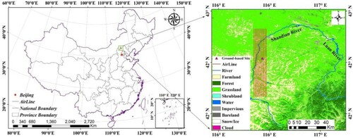
There were 11 flight lines with an interval spacing of 1 km completed within the Shandian River Basin in China, as shown in Figure 1. The main land cover type in the south is cropland, whereas in the middle north, it is grassland. The airborne active–passive microwave sensor consists of an L-band radiometer (1.41 GHz) and an L-band radar (1.26 GHz). The L-band radiometer measured both v- and h-pol brightness temperatures within a small range of incidence angles (20° to 34°) at a spatial resolution ranging from 1 to 1.4 km. The L-band radar collected backscatter data from the hh, vv, hv, and vh polarizations with incidence angles ranging from 33° to 63°. The ground spatial resolution of the radar is one-twelfth that of the radiometer, with the purpose of supporting active–passive combined downscaling. Four flights (September 17, 19, 24, and 26) were carried out in the range of 70 × 12 km (Figure 1). Due to the anomaly of the radar inertial navigation system that occurred on September 19, only the data on September 17, 24, and 26 were used in this study. According to the flight line interval of 1 km, the brightness temperature was averaged within ±1.25° of the center angles to finally form radiometer multiangular data within the range of 22.5° ∼ 32.5° (angle interval of 2.5°). The averaging of backscatter was calculated within the range of ± 5°, and finally, the multiangular radar data of 35° ∼ 55° were obtained (angle interval 2.5°). The processed multiangular radiometer and radar data were all projected onto the Equal-Area Scalable Earth (EASE) Grid 2.0 (the spatial resolutions of the radiometer and radar were 1 and 0.1 km, respectively).

Figure 1. Multiangular active-passive flights conducted during SMELR in 2018.

2.2.2. Ground-based microwave observations

The ground-based active–passive microwave observation experiment was conducted in a pasture (Xinyuan) field (∼4 km²) located in Zhenglan Banner, Inner Mongolia, China (115.93 °E, 42.04 °N). Both brightness temperature and backscatter were collected at incidence angles ranging from 30° to 65° with 2.5° intervals from August 18 to September 25, 2018. The RPG-6CH-DP radiometer was used to measure both v- and h-pol brightness temperatures in the L-, C-, and X-bands. Radar backscatter was collected using a ground-based SAR (GBSAR) at the L-, C-, and X-bands in four polarizations (vv, hh, hv, and vh). In addition, in situ measurements, including the soil moisture, surface roughness, soil temperature, and vegetation properties, were measured simultaneously over the Xinyuan pasture site.

3. Physics and methodologies

3.1. Theoretical basis for combining active–passive observations

The brightness temperature at polarization p (T_bp) and its dependency on surface characteristics is usually described using τ-ω model (Mo et al. 1982; Njoku and Entekhabi 1996). (1) $T_{bp}=T_s\cdot (1-R_p^s)\cdot \mathrm{\Gamma }+T_v\cdot (1-\omega )\cdot (1-\mathrm{\Gamma })\cdot (1+R_p^s\cdot \mathrm{\Gamma })$(1) Where T_s and T_v are the soil effective temperature and vegetation temperature. Γ is the one-way transmissivity of canopy and ω is the vegetation single scatting albedo, both of which are dependent on the vegetation characteristics. $R_p^s$ is the polarized soil reflectivity.

The soil surface to canopy thermal condition can be expected to isothermal, so that T_s≈T_v= T_e. Under low vegetation coverage, the vegetation single scatting albedo can be neglected (ω≪1) at L-band. The influence of surface roughness on soil reflectivity at L-band can be corrected using a simple parameterized model (Choudhury et al. 1979). Using these assumptions and identities, Eq. (1) becomes simply: (2) $T_{bp}=T_e\cdot (1-r_p\cdot f_1^P(roughness)\cdot {({\mathrm{\Gamma }}^P)}^2)$(2) Where r_p is the Fresnel reflectivity of a flat surface, $f_1^P$ is a function corrected for surface roughness. Solve for r_p: (3) $r_p({\theta }_1)={\displaystyle \frac{1-{\displaystyle \frac{T_{bp}}{T_e}}}{f_1^P\cdot {({\mathrm{\Gamma }}^P)}^2}}$(3) where ${\theta }_1$ is the incidence angle of radiometer, the superscript P represents parameter associated with radiometer observation.

The total radar backscatter from the land surface is attributed to three main terms: (4) ${\sigma }_{pp}^t={\sigma }_{pp}^{surf}\cdot ({\mathrm{\Gamma }}^A{)}^2+{\sigma }_{pp}^{int}+{\sigma }_{pp}^{vol}$(4) Where, the first term is the surface backscatter corrected with a two-way vegetation attenuation. The surface backscatter ${\sigma }_{pp}^{surf}$ is a function of surface roughness and Fresnel reflectivity r_p (Entekhabi et al. 2014). The second term ${\sigma }_{pp}^{int}$ is interaction between vegetation and the soil surface, which is a complex function of vegetation properties, soil roughness, and Fresnel reflectivity. The third term ${\sigma }_{pp}^{vol}$ represents the scattering from the vegetation volume, which is a complex function of vegetation characteristics. The Eq. (4) may be written as: (5) ${\sigma }_{pp}^t=f_1^A(roughness)\cdot ({\mathrm{\Gamma }}^A{)}^2\cdot r_p+f_2^A(roughness,vegetation)\cdot r_p+f_3^A(vegetation)$(5) Solve the Fresnel reflectivity r_p from Eq. (5): (6) $r_p({\theta }_2)={\displaystyle \frac{{\sigma }_{pp}^t-f_3^A}{f_1^A\cdot {({\mathrm{\Gamma }}^A)}^2+f_2^A}}$(6) where ${\theta }_1$ is the incidence angle of radar, the superscript A represents parameter associated with radar observation.

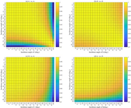
To explore the relationship between active and passive microwave observations at different angles, the relationship of Fresnel reflectivity at different angles (ranging from 0° to 65°) was analyzed under a range of volumetric soil moisture conditions (0.02 m³m⁻³–0.44 m³m⁻³). The results suggest a linear relationship between the Fresnel reflectivity at different incidence angles, and an example of the Fresnel reflectivity at 30° and 50° is shown in Figure 2. Determination coefficients (R²) between the Fresnel reflectivity h- and v-pol under all angle combinations from 0° to 65° with 2.5° intervals are shown in Figure 3. It can be seen that the linear relationship can be weakened for two distant incidence angles, and can also be weakened when approaching Brewster's angle at v-pol. The linearly relationship can be expressed: (7) $r_p({\theta }_1)=a\cdot r_p({\theta }_2)+b$(7) Consequently, the linear relationship between active and passive microwave observations at different angles still exist. A special case is that the incidence angles of radiometer and radar are the same, i.e. ${\theta }_1={\theta }_2$, $a=1$ and $b=0$. (8) $T_{bp}=T_e\cdot \left({\displaystyle \frac{a\cdot f_3^A\cdot f_1^P\cdot {({\mathrm{\Gamma }}^P)}^2}{f_1^A\cdot {({\mathrm{\Gamma }}^A)}^2+f_2^A}-b\cdot f_1^P\cdot {({\mathrm{\Gamma }}^P)}^2+1}\right)+T_e\cdot \left(-{\displaystyle \frac{a\cdot f_1^P\cdot {({\mathrm{\Gamma }}^P)}^2}{f_1^A\cdot {({\mathrm{\Gamma }}^A)}^2+f_2^A}}\right)\cdot {\sigma }_{pp}^t$(8)

Figure 2. The linear relationship between Fresnel reflectivity for different polarization combinations at incidence angle 30° and 50°.

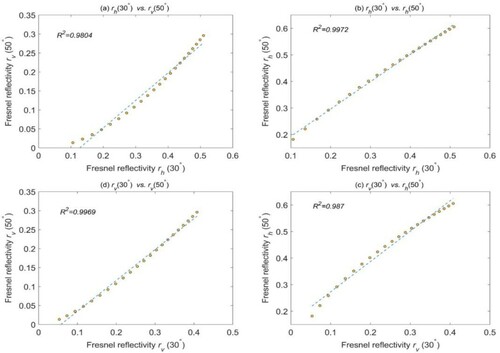
Figure 3. Determination coefficient (R²) between the Fresnel reflectivity h- and v-pol under all angle combinations from 0° to 65° with 2.5° intervals.

Thus, (9) $T_{bp}=\alpha +\beta \cdot {\sigma }_{pp}^t$(9) where $\alpha =T_e\cdot \left({\displaystyle \frac{a\cdot f_3^A\cdot f_1^P\cdot {({\mathrm{\Gamma }}^P)}^2}{f_1^A\cdot {({\mathrm{\Gamma }}^A)}^2+f_2^A}-b\cdot f_1^P\cdot {({\mathrm{\Gamma }}^P)}^2+1}\right)$, $\beta =T_e\cdot \left(-{\displaystyle \frac{a\cdot f_1^P\cdot {({\mathrm{\Gamma }}^P)}^2}{f_1^A\cdot {({\mathrm{\Gamma }}^A)}^2+f_2^A}}\right)$

3.2. The time-series regression algorithm

The downscaling algorithm proposed by Das et al. (2014) was based on the assumption of a near-linear relationship between brightness temperatures and backscatter coefficients when observed at the same incidence angle, time, and scale, which serves as the baseline downscaling algorithm for the SMAP mission. The following is a brief description of the algorithm; the full details are available in Das et al. (2014).

It is assumed that the near-linear relationship holds at all observation scales, meaning that it has the same intercept and slope parameters at coarse (C), medium (M), and fine (F) scales (resolutions). In addition, when considering the heterogeneity of vegetation and surface physical characteristics at various resolutions, the co- and cross-polarization of radar observations were introduced as indicators according to: (10) $T_{bp}(M_j)=T_{bp}(C)+\beta (C)\cdot [({\sigma }_{pp}(M_j)-{\sigma }_{pp}(C))-\mathrm{\Gamma }({\sigma }_{pq}(M_j)-{\sigma }_{pq}(C))]$(10) where T_bp(M_j), σ_pp(M_j), and σ_pq(M_j) are the brightness temperature, copolarization backscatter, and cross-polarization backscatter of pixel ‘j’ at resolution M, respectively; T_bp(C), σ_pp(C), and σ_pq(C) are the brightness temperature, copolarization backscatter, and cross-polarization backscatter at resolution C, respectively; T_bp(M_j) is the target of the active–passive downscaling algorithm, i.e. the downscaled brightness temperature; T_bp(C) is the radiometer observations collected by SMAP, which, in this study, was linearly aggregated from higher resolution radiometer observations. The values for σ_pp(M_j), σ_pq(M_j), σ_pp(C), and σ_pq(C) were obtained by aggregating higher resolution backscatter measurements within the footprints M and C. Then, β(C) can be derived from the regression of the time series of T_bp(C) and σ_pp(C), which is assumed to be time invariant within a short time period and homogeneous over entire pixels at resolution C. Γ is a seasonal sensitivity parameter for each particular pixel at resolution C, which is defined as $\mathrm{\Gamma }=[\delta {\sigma }_{pp}(M_j)/\delta {\sigma }_{pq}(M_j){]}_C$. The sensitivity parameter Γ was used to convert the heterogeneity of vegetation and surface characteristics to variations in the copolarized backscatter, and δ indicates the variation. It was estimated using copolarization and cross-polarization radar measurements through statistical regression.

3.3. Spectral analysis downscaling algorithm

The spectral analysis (SA) downscaling algorithm, which has been used to downscale satellite integrated water vapor observations, is based on a spatial field at a given resolution and can be extrapolated to higher resolution by properly estimating its spatial characteristics in the frequency domain (Montopoli, Pierdicca, and Marzano 2012). The complex Fourier spectrum F_V can be expressed by the spectral amplitude A_V and the Fourier phase ψ_V in the frequency domain of a remote sensing image: (11) $F_V(s)=A_V(s)\cdot e^{-j\cdot {\psi }_V(s)}$(11) where s is the spatial frequency, which can be calculated from the spatial wavelength (λ) by s = λ⁻¹. The power spectral density (PSD) ψ_V(s) is related to the spectral amplitude as follows: (12) ${\phi }_V(s)=|F_V(s){|}^2=[A_V(s){]}^2=s^{-v}$(12) where $⟨\cdot ⟩$ indicates the expectation operator and $|\cdot |$ is the modulus of the F_V(s). The mean PSD has a power law relationship with the spatial frequency in the Fourier frequency. v is a constant that can be obtained at coarse resolutions. For the same scalar field, the PSD of unknown resolution (M) can be inferred, at least in the averaging sense, from the empirical model of Eq. (12), which is derived from the known coarse resolution. Once the model parameters are correctly estimated, A_V of unknown resolution (M) can be resolved through Eq. (12) as the square root of the PSD. If the Fourier phase ψ_V(s) of unknown resolution (M) can also be resolved, then the Fourier spectrum F_V at an unknown resolution can be completely determined. After completely expressing the Fourier spectrum, the inversive Fourier transform is taken to recover the unknown (downscaled) field.

Montopoli, Pierdicca, and Marzano (2012) generated the Fourier phase from finer resolution interpolation using the bilinear method. However, the active–passive microwave sensors were able to collect brightness temperature and backscatter simultaneously, and a near-linear functional relationship existed between them, as described in Eq. (9). Consequently, the Fourier phase ψV of unknown resolution can be substituted by that of radar measurements obtained at a medium resolution according to the distributivity property of the 2-D Fourier transform Eq. (13). (13) $\mathrm{\Im }[a\cdot f_1(x,y)+b\cdot f_2(x,y)]=a\cdot \mathrm{\Im }[f_1(x,y)]+b\cdot \mathrm{\Im }[f_2(x,y)]$(13) where $\mathrm{\Im }$ indicates the Fourier transform. Finally, the downscaled brightness temperature is obtained through the inversive Fourier transform with a spectral amplitude A_V estimated from the brightness temperature observation at a coarse resolution and the Fourier phase ψ_V inferred from radar observations aggregated at a medium resolution. In this study, the linear aggregation method was used to aggregate radar and radiometer observations from a fine resolution to obtain a coarse or a medium resolution.

4. Results and discussion

4.1. Results from SMEX02 at the same incidence angle

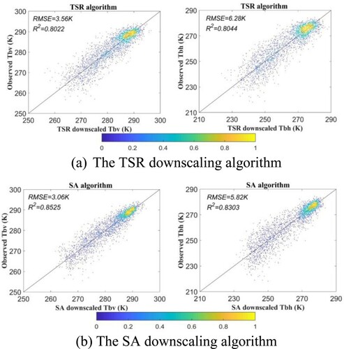
The brightness temperature downscaling algorithms were first assessed with the SMEX02 dataset with the same incidence angle at 40°. The TSR and SA downscaling algorithms were implemented to obtain the downscaled brightness temperature at ∼0.8 km. Figure 4 shows the aggregated brightness temperatures at ∼4 km (coarse resolution), gridded observations at ∼0.8 km, and downscaled brightness temperature using the TSR and SA downscaling algorithms (∼0.8 km). As observed in Figure 4, the spatial patterns of both algorithms showed a similar pattern to the original observation, which indicated that both algorithms had the ability to correctly capture the brightness temperature pattern, as shown in the observed brightness temperature. The results of the TSR algorithm also included more details, while the results from the SA method were slightly blurry or smoother. The reason for this phenomenon is that the theoretical basis of the SA algorithm is signal processing, for which the amplitudes of high-resolution measurements are estimated from the interpolation of observations at coarse resolutions in the frequency domain. The uncertainty of the estimated amplitudes results in blurry or smooth transformed images. The accuracy of the two downscaling algorithms was evaluated against the original observations in terms of their root-mean-square error (RMSE) values. For the TSR algorithm, the average RMSE values across the observed seven days were 3.56 and 6.28 K for the v- and h-pol, respectively. The average RMSE values produced by the SA algorithm were 3.06 and 5.82 K for the v- and h-pol, respectively. In comparison, the SA algorithm produced lower RMSE values, which were 0.5 and 0.46 K lower than the TSR algorithm for the v- and h-pol, respectively. Figure 5 shows the density scatter plot of observed and downscaled brightness temperatures at 0.8 km from the TSR and SA downscaling algorithms. From Figure 5 it can be seen that the density of low RMSEs produced by the SA method is more concentrated than that of the TSR method. Moreover, further evaluation of the skill of both methods was undertaken through the examination of the coefficient of determination (R²) between the downscaled and observed brightness temperatures using all seven days of data. It was noted that the determination coefficient of the SA method was 0.0503 and 0.0239 higher for both h- and v-pol, indicating that it could be an alternative method for downscaling brightness temperature.

Figure 4. Brightness temperature (T_b) of the PALS dataset during SMEX02, aggregated T_b at 4 km, observed (reference) T_b at 0.8 km, and downscaled T_b from the TSR and SA downscaling algorithms at 0.8 km: (a) v-polarization; (b) h-polarization.

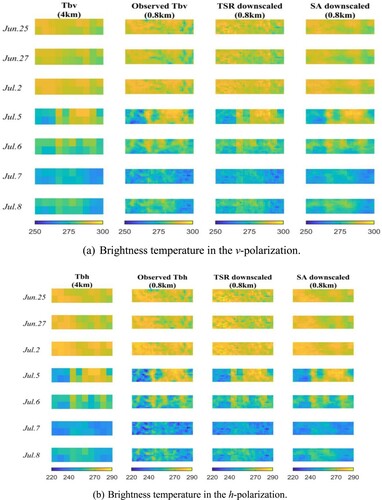
Figure 5. Comparison between the downscaled and observed brightness temperatures (T_b) resulting from the TSR and SA methods. The performance of each method was evaluated in terms of RMSE and correlation (R²) between the downscaled and reference values.

To evaluate how the time series observation pair affect the accuracy of the two downscaling algorithms, various combinations of length time series observations were used for downscaling. During the SMELR campaign, only three-day airborne active–passive microwave observations were collected. Consequently, three-day (June 27, July 5, and July 7) observations with time intervals consistent with that of SMELR were used for downscaling. With the shorter observation length, RMSE increased by 0.44 K for the h-pol and 0.26 K for the v-pol compared to the seven-day observation used. When five-day (June 27, July 2, 5, 6, and 7) observations were used, the RMSE values were 0.13 and 0.07 K higher than those based on seven-day observations. The results indicate that longer observed time periods could obtain more accurate regression results to obtain more accurate downscaling results. It was also confirmed that if there are insufficient time series observations, downscaling can still be conducted with slight reductions in accuracy.

4.2. Assumed robustness at variant incidence angles

The assumption was made that a linear relationship exists between the active and passive observations at the same incidence angle, which is the basis for downscaling brightness temperature using backscatter observations. For the case of TWRS, the incidence angles of active and passive observations varied. According to the analysis in Section3.1, the active and passive microwave observations are also approximately linear under variable angles. Therefore, the robustness of the linear relationship between brightness temperature and backscatter for the four possible polarization combinations (i.e. T_bh and σ_hh, T_bh and σ_vv, T_bv and σ_hh, T_bv and σ_vv) under all angle combinations from 30° to 65° at 2.5° intervals were investigated. To quantify the linear relationship between brightness temperature and backscatter, the determination coefficient R² was calculated using the entire time series of ground-based active and passive observations collected during the SMELR in 2018. The results for the different polarization combinations under all angle combinations are shown in Figures 6 and 7. The results showed that in most cases, the linear relationship between brightness temperature and backscatter was still robust under varying incident angle combinations. The linear correlation between T_b (both h- and v-pol) and σ_vv was stronger than that with σ_hh for most incidence angle combinations, and these results are in good agreement with those presented in previous studies (Das, Entekhabi, and Njoku 2011; Wu et al. 2014). For the pasture field, in which the vegetation contribution was quite small, the microwave emission and backscatter were dominated by the soil surface in terms of soil moisture and surface roughness. The hh polarization mode was slightly more sensitive than the vv polarization mode to soil surface roughness (Geng et al. 1996; Holah et al. 2005). Several studies have shown that vv polarization is more sensitive to soil moisture than hh polarization (Holah et al. 2005; Zhang et al. 2008; Li et al. 2014). The radiometer brightness temperature was more sensitive to soil moisture than to soil roughness in most cases. This could explain why the linear correlation between T_b (both h- and v-pol) and σ_vv is stronger than that with σ_hh for most incidence angle combinations.

Figure 6. Variability of determination coefficient (R²) values as a function of incidence angles of the radar from 30° to 65° with 2.5° intervals.

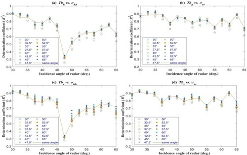
Figure 7. Determination coefficient (R²) between the L-band brightness temperature and backscatter coefficient under all angle combinations from 30° to 65° with 2.5° intervals.

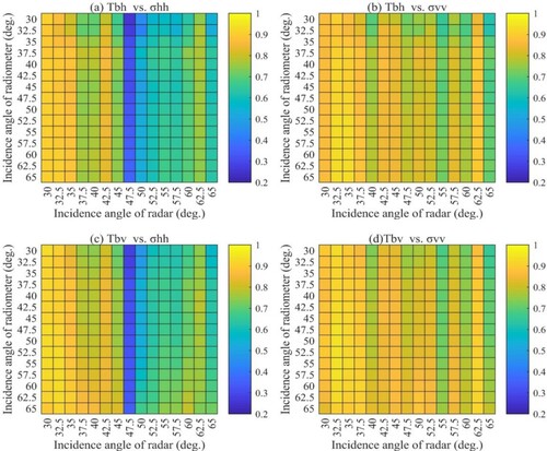
According to the experimental observations, for each incidence angle of a given brightness temperature (in both h- and v-pol), as the incidence angle of σ_hh increases, the determination coefficient (R²) first decreases and then increases with the tipping point at 47.5°. Whether this is caused by surface heterogeneity or vegetation type needs further study. The correlation between T_b (in both h- and v-pol) and σ_vv only changes slightly for each incidence angle combination. The determination coefficient (R²) between T_bh and σ_vv reaches its highest value at an active incidence angle of 32.5° for each passive incidence angle from 30° to 47.5° with a maximum determination coefficient of 0.9236 and 35° for each passive incidence angle from 50° to 65° with a maximum determination coefficient of 0.9351. The best correlation between T_bv and σ_vv occurs at an active incidence angle of 32.5° for each passive incidence angle from 30° to 62.5°, with a maximum determination coefficient (R²) of 0.9434. The determination coefficient (R²) changes slightly when the incidence angle of radar is the same for each incidence angle of T_b, which indicates that the linear relationship between active and passive observations mainly depends on the incidence angle of the radar. Therefore, both the TSR and SA downscaling algorithms were applied to demonstrate the feasibility of each when the incidence angles of the radiometer and radar are different in the next section.

4.3. Results from SMELR at different incidence angle

Using the airborne data from the SMELR dataset, the brightness temperature at 4 km (coarse resolution) was aggregated from 1 km radiometer observations, and the radar observations were aggregated from 0.1 km to 1 km (downscaling resolution) prior to applying the downscaling algorithm. Consequently, the downscaled brightness temperature results were derived at a resolution of 1 km using aggregated radar observations. As stated in section 4.2 and a previous study, the backscatter at vv-pol had the best linear correlation with brightness temperature for both h- and v-pol. Therefore, the relationships of σ_vv and brightness temperature were used to downscale the brightness temperature at h- and v-pol, respectively. Radiometer data with incidence angles of 22.5°, 25.0°, 27.5°, 30.0° and 32.5° and radar data ranging from 40.0° to 52.5° with 2.5° interval were selected for downscaling according to their consist spatial coverages. Both the TSR and SA downscaling algorithms were conducted for the nine possible incidence angle combinations (i.e. 27.5°- 40°, 27.5°- 42.5°, 27.5°- 45°, 27.5°- 47.5°, 27.5°- 50°, 25.0°- 52.5° for radiometer incidence angles of 27.5°). The observed brightness temperature at the original resolution of 1 km resolution was used as the reference to evaluate the downscaled results. The downscaling performance in terms of RMSE is presented in Table 2, and an example of intercomparing between the downscaling results and observed (reference) brightness temperature is shown in Figures 8 and 9 for the incidence angle of the radiometer at 27.5° for both h- and v-pol.

Figure 8. Brightness temperature (T_b) at an incidence angle of 27.5° from SMELR in 2018, aggregated T_b at 4 km, observed (reference) T_b at 1 km, and downscaled T_b from the TSR and SA downscaling algorithms at 1 km with incidence angle of radar backscatter at (a) 40°; (b) 42.5°; (c) 45° (d) 47.5°; (e) 50°; (f) 52. 5°.

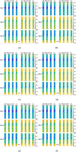
Figure 9. Comparison between observed and downscaled brightness temperatures (T_b) from the TSR and SA algorithms at various incidence angles. The performance of each method was evaluated in terms of RMSE and determination correlation (R²) between downscaled and reference T_b.

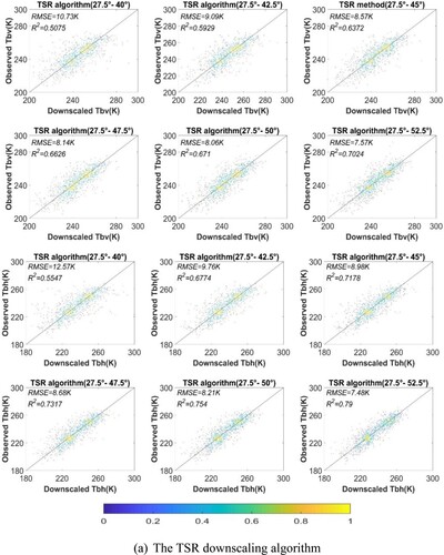
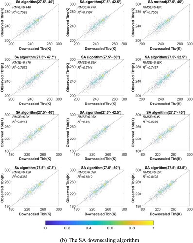
Table 2. Root mean square error (RMSE) between the downscaled brightness temperature (T_b) and reference T_b with respect to polarization and incidence angles.

	Passive Active	TSR algorithm					SA algorithm
		22.5° (K)	25.0° (K)	27.5° (K)	30.0° (K)	32.5° (K)	22.5° (K)	25.0° (K)	27.5° (K)	30.0° (K)	32.5° (K)
V	40°	11.75	11.44	10.73	11.69	11.82	5.97	5.97	6.44	6.86	7.45
	42.5°	10.71	10.19	9.09	9.60	9.40	6.05	6.06	6.47	6.65	7.37
	45°	10.34	9.82	8.57	8.51	8.18	6.04	6.07	6.49	6.67	7.48
	47.5°	10.04	9.37	8.14	8.23	7.83	6.01	6.04	6.47	6.69	7.49
	50°	9.77	9.09	8.06	8.08	7.62	5.94	6.13	6.89	7.07	7.35
	52.5°	9.17	8.42	7.57	7.48	7.09	5.95	6.12	6.88	7.03	7.3
H	40°	11.62	11.65	12.57	12.14	12.75	6.11	5.82	6.3	6.09	6.02
	42.5°	8.62	8.51	9.76	9.67	10.07	6.15	5.87	6.37	6.17	6.1
	45°	7.79	7.64	8.98	8.77	8.76	6.15	5.89	6.4	6.24	6.18
	47.5°	7.43	7.24	8.68	8.57	8.44	6.19	5.93	6.42	6.27	6.25
	50.0°	7.09	6.91	8.21	8.19	8.06	6.26	6.02	6.39	6.21	6.03
	52.5°	6.66	6.43	7.48	7.43	7.27	6.22	5.97	6.36	6.21	5.99

The results showed that both algorithms performed well when the incidence angles of the active and passive observations were different, especially for the RMSE value of the h-pol, which was consistent with that of SMEX02. The TSR algorithm is sensitive to the incidence angle of radar observation. When the radiometer angle is the same, the RMSE decreases with increasing incidence angles for radar observations. The main reason is that both co- and cross-polarization observations are used in the TSR algorithm, and the quality of radar observations is relatively good with increasing incidence angles. This can also be seen in Figure 8; with increasing radar incidence angles, the spatial pattern of the downscaling result is better. The RMSE of the SA algorithm shows no obvious change with the incidence angle. This may be because the SA algorithm only uses the phase information of radar copolarized observations in the frequency domain, so it weakens the dependence of the SA algorithm on the incidence angle. It is noted that the RMSE of the SA algorithm at 32.5° v-pol is larger than that at other angles. This is because the RFI was not completely eliminated at the boundary of the flight region in the v-pol mode on the 17th. In addition, it can also be found that both downscaling algorithms are not only dependent on the near linear relationship between the active and passive observations at variant incidence angles but are also affected by factors such as surface heterogeneity and vegetation conditions. In Eq. (9), the parameters α and β depend on vegetation and surface roughness. For the development of both downscaling algorithms, the main limitation is the assumption of a constant α and β across a coarse pixel, where α(M) = α(C) and β(M) = β(C), which should be true for a perfectly homogeneous region. However, this could not represent the real distribution of α and β due to the heterogeneity of natural surfaces. If the coarse pixel was entirely covered by homogenous vegetation, then the use of a single α and β would be appropriate for downscaling. However, variations in vegetation type, soil moisture heterogeneity, or surface roughness would result in different values of α and β for medium-resolution pixels within the same coarse pixel.

The TSR algorithm can better reproduce the spatial pattern details but has larger RMSEs with minimum values of 6.43 and 7.09 K for the h- and v-pol, respectively. The SA downscaling method could basically reflect the spatial distribution of the brightness temperature observations at 1 km, but the downscaled brightness temperature showed a blocky distribution. The reason for the blocky distribution is that averaging ($T_{bp}(C)\approx 1/nm\sum _{j=1}^{nm}{T}_{bp}(M_j)$) was carried out over nm pixels (M) to keep the disaggregated brightness temperature consistent with the radiometer brightness temperature. However, the RMSE here is lower than that of the TSR algorithm, with minimum RMSEs of 5.82 and 5.94 K for the h-pol and v-pol, respectively. In comparison, the TSR method had a larger RMSE than the SA method for both h-pol and v-pol. One possible reason for the relatively worse performance of the TSR method is the shorter time series of the airborne data in SMELR. For the TSR method, the accuracy of the downscaling results is mainly dependent on the parameter β, as shown in Eq. (9). The parameter β was estimated from the regression of the time series of active and passive observations at a coarse resolution (C), and more accurate regression requires a longer time period to make it statistically significant. However, only three days of flight data were available during the SMELR campaign, and the instability of time series regression leads to the decreased reliability of the β estimation and the reduced accuracy of the downscaling results. This indicates that the TWRS mission needs to be designed with a short orbit revisit period to ensure enough similar pairs of active–passive observations. The SA method does not need to estimate the parameter β for downscaling, which is a potential reason that the accuracy of the SA method is higher than that of the TSR method.

In addition, the mechanisms of the two downscaling methods are different. Although both methods are based on the linear relationship between active and passive microwave observations (Eq. (9)), the TSR method combines the active and passive observations based on regression analysis, which requires a satisfactory number of active–passive observations to regress the necessary parameters (β and Γ in Eq. (10)) for downscaling. However, the SA downscaling method only uses the linear relationship to combine the phase and amplitude of active and passive signals to achieve the purpose of downscaling. There is no actual linear regression analysis between active and passive observations in the process of SA downscaling. Moreover, the TSR method assumes a constant β within a coarse pixel, but the parameter β varies with respect to surface roughness and vegetation conditions. Although co- and cross-polarization backscatter was used to correct the subgrid heterogeneity effects, it was still based on statistical regression. The SA method assumes the parameter β to be constant within a medium-scale pixel, which greatly reduces the error caused by heterogeneity. This may be another reason why the RMSE of the SA method is lower than that of the TSR method. The main limitation of the SA algorithm is the ambiguity of its spatial pattern. Therefore, cross-polarization observations collected by radar instruments should be introduced to correct the effects of surface heterogeneity and vegetation and improve the availability of detailed information in downscaling results.

5. Conclusions

The objective of this study was to test the active–passive combined downscaling algorithm under variant incidence angles for application to new missions. The robustness of the two downscaling approaches, the TSR and SA methods, was evaluated using the PALS datasets from SEMX02. The algorithm was found to perform well compared to the TSR method with a lower RMSE value and a higher correlation, indicating that it can be used as an alternative method for downscaling brightness temperature. Consequently, both approaches were tested for downscaling brightness temperature under variant incidence angles using multiangular airborne data from SMELR. Before conducting the downscaling algorithm, the robustness of the active–passive linear relationship under various incidence angles was evaluated using ground multiangular active–passive observations from SMELR. The results showed that in most cases, the linear relationship between brightness temperature and backscatter was robust not only for the same incidence angle but also for varying incident angle conditions. Moreover, it was found that backscatter measured in the vv-pol was best correlated to brightness temperature at both h- and v-pol for incidence angles ranging from 30° to 65°, therefore being more suitable for downscaling brightness temperature than backscatter at hh-polarization.

Airborne active–passive observations collected at variance incidence angles were applied to both downscaling approaches. The results showed that the SA method performed better than the TSR method according to the resultant RMSE values. The downscaling spatial patterns produced by both approaches largely matched that of the reference, but the SA method exhibited obvious boundary traces inherited from coarse pixels. It was also found that the accuracy of the TSR method was primarily determined by the correlation between brightness temperature and backscatter, which required long time-series active–passive observations for reliable regression. Both assessed downscaling approaches can be applied to downscaling using the synchronous active–passive observations obtained with 1-D synthetic aperture technology under incidence angles varying between days. This study can provide support for the design of new satellite missions with passive and active observations under different incidence angles.

Disclosure statement

No potential conflict of interest was reported by the author(s).

Additional information

Funding

This work was supported by the Natural Science Foundation of Shandong Province under grant number ZR2020MD017, the Natural Science Foundation of China under grant number 41501409 and the Natural Science Foundation of Shandong Province under grant number ZR2015DL003.

References

- Akbar, R., and M. Moghaddam. 2015. “A Combined Active-Passive Soil Moisture Estimation Algorithm with Adaptive Regularization in Support of SMAP.” IEEE Transactions on Geoscience and Remote Sensing 53 (6): 3312–3324. doi:https://doi.org/10.1109/TGRS.2014.2373972.
- Anderson, M. C., J. M. Norman, J. R. Mecikalski, J. A. Otkin, and W. P. Kustas. 2007. “A Climatological Study of Evapotranspiration and Moisture Stress Across the Continental United States Based on Thermal Remote Sensing: 2. Surface Moisture Climatology.” Journal of Geophysical Research: Atmospheres 112 (D11112): 1–13. doi:https://doi.org/10.1029/2006JD007507.
- Bastiaanssen, W. G., D. J. Molden, and I. W. Makin. 2000. “Remote Sensing for Irrigated Agriculture: Examples from Research and Possible Applications.” Agricultural Water Management 46 (2): 137–155. doi:https://doi.org/10.1016/S0378-3774(00)00080-9.
- Brocca, L., L. Ciabatta, C. Massari, S. Camici, and A. Tarpanelli. 2017. “Soil Moisture for Hydrological Applications: Open Questions and New Opportunities.” Water 9 (140): 1–20. doi:https://doi.org/10.3390/w9020140.
- Choudhury, B. J., T. J. Schmugge, A. Chang, and R. W. Newton. 1979. “Effect of Surface-Roughness on the Microwave Emission from Soils.” Journal of Geophysical Research: Oceans 84 (C9): 5699–5706. doi:https://doi.org/10.1029/JC084iC09p05699.
- Corradini, C. 2014. “Soil Moisture in the Development of Hydrological Processes and Its Determination at Different Spatial Scales.” Journal of Hydrology 516: 1–5. doi:https://doi.org/10.1016/j.jhydrol.2014.02.051.
- Dai, A., K. E. Trenberth, and T. Qian. 2004. “A Global Dataset of Palmer Drought Severity Index for 1870–2002: Relationship with Soil Moisture and Effects of Surface Warming.” Journal of Hydrometeorology 5 (6): 1117–1130. doi:https://doi.org/10.1175/JHM-386.1.
- Das, N. N., D. Entekhabi, R. S. Dunbar, A. Colliander, F. Chen, W. Crow, T. J. Jackson, et al. 2018. “The SMAP Mission Combined Active-Passive Soil Moisture Product at 9 km and 3 km Spatial Resolutions.” Remote Sensing of Environment 211: 204–217. doi:https://doi.org/10.1016/j.rse.2018.04.011.
- Das, N. N., D. Entekhabi, and E. G. Njoku. 2011. “An Algorithm for Merging SMAP Radiometer and Radar Data for High-Resolution Soil-Moisture Retrieval.” IEEE Transactions on Geoscience and Remote Sensing 49 (5): 1504–1512. doi:https://doi.org/10.1109/TGRS.2010.2089526.
- Das, N. N., D. Entekhabi, E. G. Njoku, J. C. Shi, J. T. Johnson, and A. Colliander. 2014. “Tests of the SMAP Combined Radar and Radiometer Algorithm Using Airborne Field Campaign Observations and Simulated Data.” IEEE Transactions on Geoscience and Remote Sensing 52 (4): 2018–2028. doi:https://doi.org/10.1109/TGRS.2013.2257605.
- De Rosnay, P., M. Drusch, A. Boone, G. Balsamo, B. Decharme, P. Harris, Y. Kerr, T. Pellarin, J. Polcher, and J. P. Wigneron. 2009. “AMMA Land Surface Model Intercomparison Experiment Coupled to the Community Microwave Emission Model: ALMIP-MEM.” Journal of Geophysical Research: Atmospheres 114 (D05108): 1–18. doi:https://doi.org/10.1029/2008JD010724.
- Dirmeyer, P. A., and S. Halder. 2016. “Sensitivity of Numerical Weather Forecasts to Initial Soil Moisture Variations in CFSv2.” Weather and Forecasting 31 (6): 1973–1983. doi:https://doi.org/10.1175/WAF-D-16-0049.1.
- Dobriyal, P., A. Qureshi, R. Badola, and S. A. Hussain. 2012. “A Review of the Methods Available for Estimating Soil Moisture and Its Implications for Water Resource Management.” Journal of Hydrology 458–459: 110–117. doi:https://doi.org/10.1016/j.jhydrol.2012.06.021.
- Entekhabi, D., N. Das, E. Njoku, S. Yueh, J. Johnson, and J. Shi. 2014. “Soil Moisture Active Passive (SMAP) Algorithm Theoretical Basis Document: L2 &L3 Radar/Radiometer Soil Moisture (Active/Passive) Data Products.” December 9. https://smap.jpl.nasa.gov/system/internal_resources/details/original/277_L2_3_SM_AP_RevA_web.pdf.
- Entekhabi, D., E. G. Njoku, P. E. O’Neill, K. H. Kellogg, W. T. Crow, W. N. Edelstein, J. K. Entin, et al. 2010. “The Soil Moisture Active Passive (SMAP) Mission.” Proceedings of the IEEE 98 (5): 704–716. doi:https://doi.org/10.1109/JPROC.2010.2043918.
- Geng, H., Q. H. J. Gwyn, B. Brisco, J. Boivert, and R. J. Brown. 1996. “Mapping of Soil Moisture from C-Band Radar Images.” Canadian Journal of Remote Sensing 22 (1): 117–126. doi:https://doi.org/10.1080/07038992.1996.10874642.
- Guo, P., J. C. Shi, and T. J. Zhao. 2013. “A downscaling algorithm for combining radar and radiometer observations for SMAP soil moisture retrieval.” IEEE International Geoscience and Remote Sensing Symposium (IGARSS), Melbourne, 21–26 July. doi:https://doi.org/10.1109/IGARSS.2013.6721261.
- Holah, N., N. Baghdadi, M. Zribi, A. Bruand, and C. King. 2005. “Potential of ASAR/ENVISAT for the Characterization of Soil Surface Parameters Over Bare Agricultural Fields.” Remote Sensing of Environment 96: 78–86. doi:https://doi.org/10.1016/j.rse.2005.01.008.
- Kerr, Y. H., P. Waldteufel, J. P. Wigneron, S. Delwart, F. Cabot, J. Boutin, M. J. Escorihuela, et al. 2010. “The SMOS Mission: New Tool for Monitoring key Elements of the Global Water Cycle.” Proceedings of the IEEE 98 (5): 666–687. doi:https://doi.org/10.1109/JPROC.2010.2043032.
- Kim, Y., and J. van Zyl. 2009. “A Time-Series Approach to Estimate Soil Moisture Using Polarimetric Radar Data.” IEEE Transactions on Geoscience and Remote Sensing 47 (8): 2519–2527. doi:https://doi.org/10.1109/TGRS.2009.2014944.
- Koster, R. D., P. A. Dirmeyer, Z. Guo, G. Bonan, E. Chan, P. Cox, C. Gordon, S. Kanae, E. Kowalczyk, and D. Lawrence. 2004. “Regions of Strong Coupling Between Soil Moisture and Precipitation.” Science 305 (5687): 1138–1140. doi:https://doi.org/10.1126/science.1100217.
- Li, Y. Y., K. Zhao, J. H. Ren, Y. L. Ding, and L. L. Wu. 2014. “Analysis of the Dielectric Constant of Saline-Alkali Soil Sand the Effect on Radar Backscattering Coefficient: A Case Study of Soda Alkaline Saline Soils in Western Jilin Province Using RADARSAT-2data.” The Scientific World Journal 2014 (563015): 1–14. doi:https://doi.org/10.1155/2014/563015.
- Loew, A., T. Stacke, W. Dorigo, R. D. Jeu, and S. Hagemann. 2013. “Potential and Limitations of Multidecadal Satellite Soil Moisture Observations for Selected Climate Model Evaluation Studies.” Hydrology and Earth System Sciences 17 (9): 3523–3542. doi:https://doi.org/10.5194/hess-17-3523-2013.
- Massari, C., T. Moramarco, Y. Tramblay, and J. F. D. Lescot. 2014. “Potential of Soil Moisture Observations in Flood Modelling: Estimating Initial Conditions and Correcting Rainfall.” Advances in Water Resources 74: 44–53. doi:https://doi.org/10.1016/j.advwatres.2014.08.004.
- Mo, T., B. J. Choudhury, T. J. Schmugge, J. R. Wang, and T. J. Jackson. 1982. “A Model for Microwave Emission from Vegetation-Covered Fields.” Journal of Geophysical Research: Ocean 87 (C13): 11229–11237. doi:https://doi.org/10.1029/JC087iC13p11229.
- Montopoli, M., N. Pierdicca, and F. S. Marzano. 2012. “Spectral Downscaling of Integrated Water Vapor Fields from Satellite Infrared Observations.” IEEE Transactions on Geoscience and Remote Sensing 50 (2): 415–428. doi:https://doi.org/10.1109/TGRS.2011.2161996.
- Narayan, U., V. Lakshmi, and T. J. Jackson. 2006. “High-resolution Change Estimation of Soil Moisture Using L-Band Radiometer and Radar Observations Made During the SMEX02 Experiments.” IEEE Transactions on Geoscience and Remote Sensing 44 (6): 1545–1554. doi:https://doi.org/10.1109/TGRS.2006.871199.
- Njoku, E. G., and D. Entekhabi. 1996. “Passive Microwave Remote Sensing of Soil Moisture.” Journal of Hydrology 184 (1-2): 101–129. doi:https://doi.org/10.1016/0022-1694(95)02970-2.
- Njoku, E. G., W. J. Wilson, S. H. Yueh, S. J. Dinardo, F. K. Li, T. J. Jackson, V. Lakshmi, and J. Bolten. 2002. “Observations of Soil Moisture Using a Passive and Active low-Frequency Microwave Airborne Sensor During SGP99.” IEEE Transactions on Geoscience and Remote Sensing 40 (12): 2659–2673. doi:https://doi.org/10.1109/TGRS.2002.807008.
- Ochsner, T. E., M. H. Cosh, R. H. Cuenca, W. A. Dorigo, C. S. Draper, Y. Hagimoto, Y. H. Kerr, E. G. Njoku, E. E. Small, and M. Zreda. 2013. “State of the Art in Large-Scale Soil Moisture Monitoring.” Soil Science Society of America Journal 77 (6): 1888–1919. doi:https://doi.org/10.2136/sssaj2013.03.0093.
- Peng, J., A. Loew, O. Merlin, and N. E. Verhoest. 2017. “A Review of Spatial Downscaling of Satellite Remotely Sensed Soil Moisture.” Reviews of Geophysics 55 (2): 341–366. doi:https://doi.org/10.1002/2016RG000543.
- Piles, M., D. Entekhabi, and A. Camps. 2009. “A Change Detection Algorithm for Retrieving High-Resolution Soil Moisture from SMAP Radar and Radiometer Observations.” IEEE Transactions on Geoscience and Remote Sensing 47 (12): 4125–4131. doi:https://doi.org/10.1109/TGRS.2009.2022088.
- Robinson, D., C. Campbell, J. Hopmans, B. Hornbuckle, S. B. Jones, R. Knight, F. Ogden, J. Selker, and O. Wendroth. 2008. “Soil Moisture Measurement for Ecological and Hydrological Watershed-Scale Observatories: A Review.” Vadose Zone Journal 7 (1): 358–389. doi:https://doi.org/10.2136/vzj2007.0143.
- Sabaghy, S., J. P. Walker, L. J. Renzullo, and T. J. Jackson. 2018. “Spatially Enhanced Passive Microwave Derived Soil Moisture: Capabilities and Opportunities.” Remote Sensing of Environment 209: 551–580. doi:https://doi.org/10.1016/j.rse.2018.02.065.
- Saha, S., S. Moorthi, H. L. Pan, X. Wu, J. Wang, S. Nadiga, P. Tripp, et al. 2010. “The NCEP Climate Forecast System Reanalysis.” Bulletin of the American Meteorological Society 91 (8): 1015–1058. doi:https://doi.org/10.1175/2010BAMS3001.1.
- Seneviratne, S. I., T. Corti, E. L. Davin, M. Hirschi, E. B. Jaeger, I. Lehner, B. Orlowsky, and A. J. Teuling. 2010. “Investigating Soil Moisture–Climate Interactions in a Changing Climate: A Review.” Earth-Science Reviews 99 (3-4): 125–161. doi:https://doi.org/10.1016/j.earscirev.2010.02.004.
- Sheffield, J., G. Goteti, F. Wen, and E. F. Wood. 2004. “A Simulated Soil Moisture-Based Drought Analysis for the United States.” Journal of Geophysical Research: Atmospheres 109 (D24108): 1–19. doi:https://doi.org/10.1029/2004JD005182.
- Wigneron, J. P., T. J. Jackson, P. O’Neill, G. De Lannoy, P. de Rosnay, J. P. Walker, P. Ferrazzoli, et al. 2017. “Modelling the Passive Microwave Signature from Land Surfaces: A Review of Recent Results and Application to the L-Band SMOS & SMAP Soil Moisture Retrieval Algorithms.” Remote Sensing of Environment 192: 238–262. doi:https://doi.org/10.1016/j.rse.2017.01.024.
- Wu, X., J. P. Walker, N. N. Das, R. Panciera, and C. Rudiger. 2014. “Evaluation of the SMAP Brightness Temperature Downscaling Algorithm Using Active-Passive Microwave Observations.” Remote Sensing of Environment 155: 210–221. doi:https://doi.org/10.1016/j.rse.2014.08.021.
- Zhan, X. W., P. R. Houser, J. P. Walker, and W. T. Crow. 2006. “A Method for Retrieving High-Resolution Surface Soil Moisture from Hydros L-Band Radiometer and Radar Observations.” IEEE Transactions on Geoscience and Remote Sensing 44 (6): 1534–1544. doi:https://doi.org/10.1109/TGRS.2005.863319.
- Zhang, T., Q. Zeng, Y. Li, and Y. Xiang. 2008. “Study on Relation between InSAR Coherence and Soil Moisture.” The International Archives of the Photogrammetry, Remote Sensing and Spatial Information Sciences Part B XXXVII (7): 1–5.
- Zhao, T., L. Hu, J. Shi, H. Lv, S. Li, D. Fan, P. Wang, D. Geng, C. S. Kang, and Z. Zhang. 2020b. “Soil Moisture Retrievals Using L-Band Radiometry from Variable Angular Ground-Based and Airborne Observations.” Remote Sensing of Environment 248 (111958): 1–18. doi:https://doi.org/10.1016/j.rse.2020.111958.
- Zhao, T. J., J. C. Shi, L. Q. Lv, H. X. Xu, D. Q. Chen, Q. Cui, T. J. Jackson, et al. 2020a. “Soil Moisture Experiment in the Luan River Supporting New Satellite Mission Opportunities.” Remote Sensing of Environment 240 (111680): 1–20. doi:https://doi.org/10.1016/j.rse.2020.111680.