Constant-level spatio-temporal integrated search algorithm for repeating sun-synchronous orbit satellite images

ABSTRACT

Metadata information and catalogue services are major ways of making satellite images findable and accessible. Spatio-temporal indexing is the key to ensuring efficient searches. Because spatial information and temporal information are usually independently maintained and indexed, the image retrieval process has to include two search steps: a spatial query and a temporal query. As most Earth Observation satellites are specially designed to have repeating sun-synchronous orbits (RSSO), this type of satellite data has a close correlation between its spatial coverage and temporal coverage information. In this paper, an integrated spatio-temporal indexing mechanism is proposed for RSSO satellites. The spatio-temporal Look-Up Table (st-LUT) that serves as the index reflects the coupled correlation between the spatial and temporal coverage information within one orbit revisiting cycle. Image retrieval algorithms are designed based on the st-LUT. In this study, 1,765,797 Landsat 8 scenes collected from 28 June 2013 to 31 December 2019 data are used to establish and validate the proposed indexing mechanism and search algorithms. Because this new method only need to focus on the changes of the spatial and temporal coverage over the time in one orbit revisiting cycle, the spatial search space is limited to the fixed number of grids. Therefore, the search algorithm is at a constant level. Its performance is not related to the volume of the images that need to search.

GRAPHICAL ABSTRACT

KEYWORDS:

• Earth observation
• data acquisition
• remote sensing
• spatial data infrastructure
• image retrieval

1. Introduction

The global Earth observation programs have successfully acquired a huge volume of satellite image data over the last several decades. For example, the United States Geological Survey’s (USGS) Landsat data archive currently contains more than 5.5 million images (Wulder et al. 2016), and the Landsat program collects about 1 terabyte of data each day (Baumann et al. 2016). Remote sensing provides a very unique capability to constantly monitor the Earth System and its changes over the time at global scale. It has been widely utilized in many research fields, and promoted by many global organization and international collaboration projects. For example, the Group on Earth Observations (GEO) is promoting the global sharing of remote sensing data, and utilizing them to many latest global engagement priorities, such as Sustainable Development Goals (SDGs), Climate Action, and Disaster Risk Reduction. In particular, the 2030 Agenda (Cf 2015) explicitly declared to support developing countries by ensuring access to high-quality, timely, reliable, and disaggregated data, including geospatial and Earth observation data(UN 2015). In climate change studies, remote sensing images help us understand the climate system and its changes, including changes in global warming, snow and ice, sea-level changes, solar radiation, aerosols, clouds, water vapor, and precipitation (Yang et al. 2013). In addition, in terms of disaster risk reduction and monitoring, remote sensing provides fast responses. For example, the International Charter ‘Space and Major Disasters’ (Charter 2021) oversees the acquisition and transmission of satellite data to relief organizations in the event of a major disaster.

The very first step to utilize remote sensing data in many application areas is finding data of interest. With the introduction of the FAIR Data Principles (Wilkinson et al. 2016), the importance of findability has been further emphasized in the remote sensing society. For many large-scale remote sensing data centers, machine-readable metadata has been extensively utilized to enable the discovery of datasets and services to meet users’ needs. To find data of interest from such a huge archive of remote sensing images, researchers usually perform spatio-temporal queries to select the data to be processed. For example, when executing satellite image fusion tasks (Zhu et al. 2016), the ability to quickly find the overlap between two satellites is important. Moreover, in emergency response when every second counts, the ability to perform fast data queries is critical. One typical example is the Charter, which needs to coordinate satellite resources to ensure rapid response to major disaster situations. On 17 May 2019, a flood occurred in Paraguay, and the Charter member Secretaria de Emergencia Nacional (SEN) requested activation. Thirty-four remote sensing data products captured during the period from 14 May to 2 June 2019 were provided by other Charter members. The Charter members depend heavily on an efficient spatio-temporal search capability to fulfill data requests in a very timely manner.

For remote sensing image data, catalogue services (Bai and Di 2011; Bai et al. 2012) are the major mechanism used to facilitate the query process on the web. Catalogue services support the ability to publish and search collections of descriptive information (metadata) in remote sensing image data and related information objects. When performing a spatio-temporal query, the spatial operations usually account for most of the duration of the query process. Therefore, many types of spatial indexes are developed to accelerate the retrieval process. R-tree (Nascimento and Silva 1998) is a common indexing scheme derived from the B-tree (Bayer and McCreight 2002). It was originally proposed for organizing spatial objects that use multi-dimensional indexes. The R-tree and its families, such as the R⁺-Tree (Sellis, Roussopoulos, and Faloutsos 1987), the R*-Tree (Beckmann, Kriegel, and Seeger 1990), and the Hilbert R-Tree (Kamel and Faloutsos 1993), have been extensively used by researchers to conduct efficient processing of queries in multi-dimensional data sets (Manolopoulos et al. 2010). The Quadtree (Finkel and Bentley 1974) was invented by Finkel and Bentley to express an extension of the Binary Search Tree in two dimensions, which was able to index points (Point Quadtree). Then, several Quadtree variations were developed for almost all types of spatial data (Klinger and Dyer 1976; Gargantini 1982; Samet 1990). The geohashes index is another important spatial indexing model. It was invented by Gustavo Niemeyer in 2008 to geocode specific points as a short string for use in web URLs (Uniform Resource Locators). All of these indexes have been extensively applied in most relational databases to index spatial data. However, most databases cannot directly support spatio-temporal data retrieval. To realize efficient spatio-temporal queries, several indexing mechanisms have been introduced for relational databases (Tao, Papadias, and Sun 2003 Zhu, Gong, and Zhang 2007;). For example, Carvalho, Ribeiro, and Augusto Sousa (2006) developed a spatio-temporal database system based on the temporal TimeDB and Oracle Spatial for temporal and spatial support. Zhao et al. (2011) developed the Spatio-Temporal Object Cartridge (STOC), which is an Oracle-based spatio-temporal information management system. Mahmood et al. (2017) introduced the spatio-temporal ontological concept using a relational data model for modeling spatio-temporal data. For non-relational databases, Fox et al. (2013) described a spatio-temporal index structure that leverages the horizontal scalability of NoSQL databases (Accumulo) (Cordova, Rinaldi, and Wall 2015), which is a sorted, distributed, and key/value store designed for non-relational databases built on Google’s BigTable database model (Chang et al. 2008), in order to achieve performant query and transformation semantics.

All of the aforementioned spatio-temporal data indexing mechanisms maintain the spatial and temporal data independently. The spatial and temporal query constraints are executed individually. Thus, it is not easy to improve their execution efficiencies by optimizing the query constraints. Moreover, there is usually a two-level filter to execute spatial queries. The primary filter returns a superset of objects’ bounding boxes, and the secondary filter applies boundary coordinates to obtain the final result set. Therefore, there are two major limitations when retrieve remote sensing images. One is the large and increasing search space. For example, the latest Landsat 8 Operational Land Imager (OLI) and Thermal Infrared Sensor (TIRS) Collection1 Level-1 dataset contained more than 1,850,000 scenes as of 6 Sep 2020. It does take some time to find the data of interest among these millions of scenes that match multiple query criteria, such as spatial location, temporal information, and cloud coverage. In addition, all of the abovementioned methods build their index based on the entire dataset. As new data are added, the indices need to be updated, which requires extra computation and adversely affects the performance. The other limitation is the unavoidably complex spatial operations, such as intersection, containment, and distance (Arce, Bacca, and Paredes 2009), which further lead to the overall high time consumption. Because the query algorithm is executed for time and space independently (Bai et al. 2007), the total time cost is mostly dependent on the more complex one, which is usually the spatial operations. The computation time becomes unpredictable for extreme large data volumes. Considering the rapid increase in the capabilities of civilian satellite observations, the efficiency of the currently used spatio-temporal retrieval algorithms is facing great challenges, especially in the realization of the findability requirement of the FAIR principles for massive global remote sensing images.

The purpose of this study is to present a new spatio-temporal integrated indexing mechanism and a new querying method for repeating sun-synchronous orbiting (RSSO) satellite data. According to the World Meteorological Organization’s (WMO) Observing Systems Capability Analysis and Review (OSCAR) database, among the 780 satellites used for meteorological and Earth observation purposes, as of 6 Sep 2020, 451 were RSSO satellites (Oscar 2019). In addition, most of the widely used satellite data are RSSO satellite image data, such as Landsat series, Sentinel-2, QuickBird, China–Brazil Earth Resources Satellite (CBERS), and FengYun. RSSO satellites have the characteristics of both sun synchronization and repeat orbits. Therefore, they can ensure stable illumination conditions and periodic monitoring of the Earth’s surface to examine environment changes over time. An index specially designed for these RSSO satellites would improve the retrieval process and lower the maintenance costs. The current indexing methods are designed for more general purposes. They have been widely implemented in remote sensing image data management systems such as the General Index Framework for Space Partitioning Trees (SP-GiST) indexing system for the PostgrelSQL database. The revisiting characteristics of RSSO satellites have already been clearly examined by other researchers (Zhang and Roy 2016b; Li and Roy 2017), but no one has utilized this characteristic in the image retrieval process. The main reason for this is the irregular revisiting time variation. In this study, the spatio-temporal distribution of scenes and the deviation in the scene revisiting time of the RSSO satellite were studied in order to improve the robustness of the algorithm.

The rest of this paper is organized as follows. The Landsat 8 satellite image data are taken as an example, and in Section 2, the revisiting time and scene durations of all of the historical image data are analyzed. In Section 3, a spatio-temporal Look-Up Table (st-LUT) is introduced as a spatio-temporal integrated index for RSSO satellite image data. Then, based on the st-LUT, a spatio-temporal query algorithm is developed. Section 4 provides examples of three query scenarios and their corresponding retrieval results. Then, the performance of the method is analyzed. The limitations and future challenges are discussed in Section 5.

2. Data

Landsat 8 is an RSSO satellite with an orbit revisiting cycle of 16 days, which means the satellite revisits the same locations at almost the same local time every 16 days. Based on this characteristic, the World Reference System (WRS) was designed as a global notation system that catalogs the Landsat data using Path and Row numbers (NASA 2020). Because the observatory instruments onboard Landsat continually scan the Earth, the resulting data are segmented into individual frames of data that are known as scenes. The Path and Row numbers are designated to specify the nominal center of each scene, and two successive scenes are designed to occupy 23.92 s of spacecraft time calculated from the equator.

Each Landsat 8 scene has a metadata file containing its spatial coverage and temporal information. The temporal information includes the acquisition date, beginning time (the corresponding time when the scene starts to be recorded), end time (the corresponding time when the recording ends), and product generated date. The time information is defined in Coordinated Universal Time (UTC) and local time. The spatial information includes the coordinates of the four corners and the center of the scene and the corresponding path and row numbers.

Landsat 8 scenes are identified by a designated ID that follows the convention shown below. $Lxss+ppp+rrr+YYYY+DDD+GGG+VV\mathrm{\_}FT,$where L denotes the Landsat; x indicates which sensor collected the data for this product (O for OLI, T for TIRS, and C for a combination of TIRS and OLI); ss is the satellite number (e.g. 08 denotes Landsat 8); ppp is the three-digit WRS-2 path number; rrr is the three-digit WRS-2 row number; YYYY and DDD are the year and the date of acquisition, respectively; GGG is the ground station identifier; VV is the version of the algorithm used to produce the current scene; and FT is the file type (B1-B11 for image band file number, MTL for metadata file, BQA for quality band file, and MD5 for checksum file).

Although Landsat 8 images are available starting from 9 March 2013, the operational status was not fully established until late June. In this study, scene 100–11 (in this paper, Path and Row information is given in the format of Path-Row) taken on 28 June 2013 was considered to be the first scene when the revisiting time became stable. The exact beginning acquisition time of this scene is introduced as T₀ (time stamp). The time is 2013:179:00:24:42 in the year:day:hour:min:sec format, and the time stamp is 1372350282.

In this study, the Landsat 8 historical scenes were divided into two parts. All of the 1,765,797 scenes collected from 28 June 2013–31 December 2019 were used to establish the new spatio-temporal integrated indexing mechanism and the new querying method. The rest of the scenes, i.e. those acquired since 2020, were used for testing.

3. Methods

3.1. Building the spatio-temporal look-up table

The basic idea of an st-LUT focused on one repeating cycle to infer other spatio-temporal locations. The pattern was calculated and formatted into a table, which is called a spatio-temporal look-up table (st-LUT; Figure 1) for Landsat 8. Table 1 illustrates the table’s structure.

Figure 1. The relationship between the spatio-temporal look-up table and the scenes.

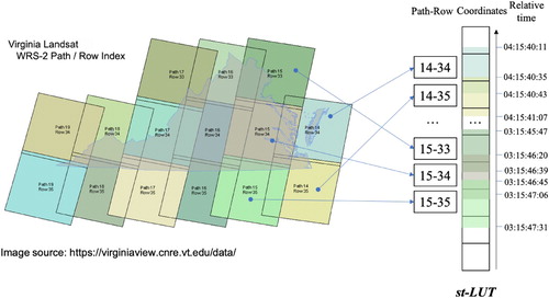
Table 1. Example of a spatio-temporal look-up table for Landsat 8.

ID	Coordinates	WRS-2 Path	WRS-2 Row	Temporal duration field
1	(UL, UR, LL, LR^a)100-11	100	11	[T(100-11)b, T(100-11)e]
2	(UL, UR, LL, LR)100-12	100	12	[T(100-12)b, T(100-12)e]
…
	(UL, UR, LL, LR)i−j	i	j	[T(i−j)b, T(i−j)e]
…
233*248	(UL, UR, LL, LR)100-10	100	10	[T(100-10)b, T(100-10)e]

^a UL: Upper left coordinate; UR: Upper right coordinate; LL: Lower left coordinate; LR: Lower right coordinate.

For Landsat 8 scene archive $\mathrm{{\rm Y}}$, every path-row location has a time series of scenes ${\mathit{S}}^{ij}=\left[S_1^{ij},\dots ,S_n^{ij}\right]n\in \mathit{R}$, where i is the path number and j is the row number. These series $S_1^{ij},\dots ,S_n^{ij}$contain both the historical and future scenes of this path-row location, and n denotes the number of the scene in time order.

In the st-LUT, the records are listed in time order, i.e. according to the flying track of the Landsat 8. Each st-LUT record consists of two spatial fields (a WRS-2 number field and a corner coordinates field) and the temporal duration field. The temporal duration field is the time cost of the satellite records for each scene. It always records from the same relative time in every revisiting cycle. This field is expressed by a time pair [T_(ij)b, T_(ij)e] where T_(ij)b is the scene’s beginning time in Path-Row i-j in a 16-day cycle (T_(ij)b is calculated using Equations (1.2) and (2)). Similarly, T_(ij)e is the scene’s end time in Path-Row i-j in a 16-day cycle.

The temporal duration field of the st-LUT is the average number of each scene’s relative time in one revisiting cycle. The decimal number p is introduced to denote the time position of a UTC time since T₀ (see Equation (1.1)). The relative time t represents the time offset within one revisiting cycle, which is scaled to [0,16] (see Equation (1.2)). The integer n is the cycle’s ordinal number of ut since T₀. For the convenience of calculation, all of the UTC times were converted to timestamps (time in second). (1.1) $p=\frac{ut-T_0}{T}.$(1.1) (1.2) $t=\frac{\mathrm{m}\mathrm{o}\mathrm{d}\left(ut-T_0,T\right)}{T}\cdot T_d.$(1.2) (1.3) $n=\frac{ut-T_0}{T}.$(1.3) Sz is the length of the orbit revisit cycle (in seconds). T₀ was introduced in Section 2 in this paper. For Landsat 8, the revisiting cycle is 16 days. The cycle in days T_d is equal to 16, and the cycle in seconds T is equal to 1382400. Using Equation (1.2), every beginning and end time of ${\mathit{S}}^{ij}$ can be converted to a relative time ${\mathit{t}}^{ij}=\left[\left(t_{1b}^{ij},t_{1e}^{ij}\right),\dots ,\left(t_{nb}^{ij},t_{ne}^{ij}\right)\right],n\in \mathit{R}$.

The expectation of the historical beginning and end times of ${\mathit{t}}^{ij}$ (see Equation (2)) represents the average level of the revisiting time. This is considered to be the basis of the st-LUT’s temporal duration field. (2) $\left\{\begin{array}{c}{T}_{\left(ij\right)b}=E\left({\mathit{t}}_b^{ij}\right)\\ T_{\left(ij\right)e}=E\left({\mathit{t}}_e^{ij}\right)\end{array}\right..$(2) The relative time t can also be extended to the n^th timestamp $u{t}_n$ using Equation (3). (3) $u{t}_n=t\cdot T+\left(n-1\right)\cdot T+T_0.$(3) n denotes the n^th cycle starting from T₀. Equation (3) not only provides the ability to calculate all of the possible time locations, but it also provides the possibility of developing a future image acquisition plan when the n is set to a number larger than the current cycle.

3.2. The deviation of the time field

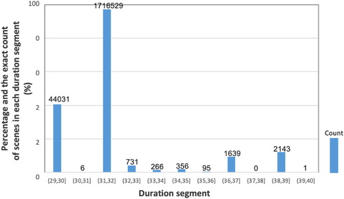
Figure 2 describes the fluctuation in the scene duration segment. For Landsat 8, each scene will ideally last for 32 s, so that it will revisit the same place at the same local time. Generally speaking, it takes 31 or 32 s to record one scene, but about 2% of the scenes last for approximately 29 s and less than 0.3% of the scenes last for more than 32 s. This leads to a deviation in the revisiting time at each Path-Row location. For example, one scene was recorded starting at 01:06:47 on 22 April 2019 at location 104/61. The next time Landsat 8 revisited location 104/61 should have started at 01:06:47 on 8 May 2019. However, scene 104/61 was actually captured at 01:06:52 on 8 May 2019, which is 5 s later than the planned revisit. This slight difference in time is mainly related to the orbit’s altitude and inclination drift (Wertz 2001; Zhang and Roy 2016a), which are caused by many factors, such as gravitational factors. Thus, the satellite needs to keep maneuvering to maintain its orbit (Wertz 2001).

Figure 2. Distributions of the durations of the historical Landsat 8 scenes.

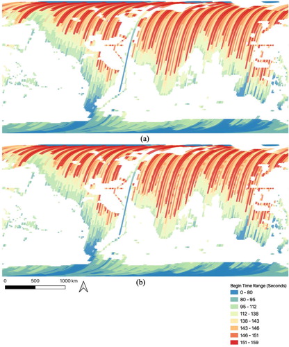
Because orbit drift and maneuvers cannot be precisely predicted for future acquisition, we set a buffer for the temporal duration field in order to include all of the possible results when implementing the retrieval algorithm. In order to determine the buffer window setting, Figure 3(a) and (b) plot the deviation in every Path-Row’s revisiting time comparing with the average value. The absolute value of the time difference ranges from 0 to 160 s. Geographically speaking, the revisiting time deviations in most areas between latitude 60°N and 90°S are relatively small, i.e. less than 140 s, but the revisiting time (both of beginning and end time) of scenes taken along some paths deviate by up to 160 s. Setting a proper time buffer can help to improve the coverage of the st-LUT’s temporal field and to improve the robustness of the algorithm. According to the deviation, the buffer window was set to 160 s for each time boundary, so the full window was 320 s wide. Therefore, the temporal duration field time pair calculated using Equation (2) extended to [T_(ij)b−160T_d/T, T_(ij)e + 160T_d/T] for Landsat 8.

Figure 3. The revisiting time deviation range compared with the average revisiting time for each Path-Row. (a) Plot of beginning time deviation range; and (b) plot of end time deviation range.

3.3. The design of the retrieval algorithm

The retrieval algorithm consists of three parts: temporal query, spatial query, and spatio-temporal query algorithms. The st-LUT is the basis of these algorithms.

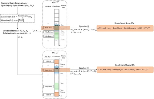
3.3.1. Temporal query algorithm

Algorithm A (Figure 4) shows the steps required to fulfill a temporal query.

Figure 4. Algorithm A of the temporal query.

Problem Statement. Given the time query constraint (qt_b, qt_e) where qt_b<qt_e, the algorithm returns the corresponding records intersecting with the temporal constraints and all possible scene IDs.

The time location of the query constraint and the relative time in the cycle are (p_b, p_e) and (t_b, t_e), respectively, and they are obtained using Equation (1.1) and Equation (1.2). The ΔD is the time duration of the input time constraint $\left(\mathrm{\Delta }D=p_e-p_b\right)$. According to the value of ΔD, there are several possible situations.

1. If ΔD ≤ 1, the time duration is less than one orbit cycle. Thus, there is no repeating location in the result set. The simplest situation is when t_e > t_b, for which the time constraint falls within the same cycle. The algorithm directly takes (t_b, t_e) as the input to the st-LUT for the query. Algorithm A returns a result set of Path-Rows whose time fields intersect with (t_b, t_e) according to the st-LUT. However, when t_e < t_b, the time query constraint crosses the boundary of a cycle. The time t_b is near the end of a cycle and t_e is near the start of the next cycle. The result set contains a group of Path-Rows whose temporal fields intersect with (t_e, 16) and (0, t_b) according to the st-LUT.

2. If ΔD > 1, the query covers at least one full cycle. Therefore, every path-row location is visited at least once. The (p_b, p_e) can be divided into several relative time periods using the integer part, e.g. (p_b, n), [n + 1, n + 2), [n + 2, p_e). The integer part n is the n^th cycle starting at T₀. The query result will return a large set of records covering the entire surface of the Earth between times qt_b and qt_e.

The result records obtained using Algorithm A contain both Path-Row and relative time information. The relative time information should be converted back into UTC time using Equation (3). Then, the result sceneIDs can be concatenated with the Path-Row and UTC time information. The result may be a superset due to the buffer setting. Other specific information can be applied for further filtering.

3.3.2. Spatial query algorithm

The Algorithm B (Figure 5) describes how to filter qualified results using spatial constraints. With only spatial constraints, the result set will be a time series of images.

Figure 5. Algorithm B of the spatial query.

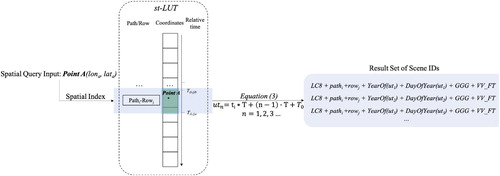
Problem Statement. Given the spatial information, i.e. [Path₁-Row₁, Path₂-Row₂, … , Path_n-Row_n] or [point₁, point₂, … , point_n], the algorithm returns the corresponding records intersecting with the spatial constraints and all possible scene IDs.

1. If the spatial information is in the Path-Row format, the result records can be selected by looking up the st-LUT. The result records include the spatial and temporal information for the string concatenation of SceneID. The temporal field needs to be extended to a UTC time sequence (ut₁, ut₂, ut_3, … , ut_n) using Equation (3). In this case, there are no time constraints. Therefore, the time sequence can include all of the potential imaging times from past to future by adjusting the cycle number n. Then, a string concatenation of the given spatial information and the resulting time sequence is applied to retrieve the final sceneIDs.

2. If the spatial information is in the coordinate format, the retrieving process needs to be conducted using the ‘coordinates’ column of st-LUT. A spatial index is necessary to accelerate the spatial query. Although this algorithm still involves spatial operations, it compresses the search space compared to traditional spatial queries. The spatial index is only necessary to build on the st-LUT, which only contains the coordinates in one revisiting cycle.

Similar to Algorithm A, the relative time information of the result records should be converted back to UTC time using Equation (3). The result sceneIDs can be concatenated with the path-row and UTC time information. The result may be a superset due to the buffer setting. Other specific information can be applied for further filtering.

3.3.3. Spatio-temporal query algorithm

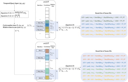
Algorithms A and B are performed based only on spatial or temporal constraints, respectively. When a query involves both spatial and temporal information. The retrieval process follows Algorithm C (Figure 6).

Figure 6. Algorithm C of the spatio-temporal query.

Algorithm C is for both temporal and spatial queries. The spatial and temporal queries will be conducted based on the st-LUT. Therefore, the computational load will be smaller than the traditional database query processes due to the coupled spatio-temporal property.

For example, if it receives (qt_b, qt_e) as the temporal constraint and (lon_a, lat_a) as the spatial constraint, the spatial information helps to locate the Path-Row number of the candidate set, and temporal information filters the final result set using Equation (3) by providing the number of cycles since T₀.

This process not only reduces the search space for spatial queries from the full set to a limited table volume, which will not exceed the size of the st-LUT, but it also avoids a second search of the time field using Equation (3).

However, RSSO satellites do not recording the entire surface of the Earth all the time, instead they record certain areas according to their mission and operation status. Therefore, some concatenated sceneIDs may not obtain scenes. These sceneIDs will return empty when retrieving scenes from physical file systems.

3.4. Time cost

By taking advantage of the orbit revisiting characteristic, the search space is compressed into one orbital cycle, and it is not related to the volume of the datasets. Therefore, the computational time of the proposed algorithm should remain almost the same regardless of the size of the test set.

In order to test the query performance under different data volumes, the Landsat historical scene metadata were reorganized as four subsets containing 10000, 100000, 1000000, and 1850000 scenes, respectively. One hundred spatio-temporal query constraints were randomly generated as the query inputs and each query was executed three times as the time cost of this query to avoid some extreme situations. The average computational time of the one hundred queries was defined as the final computational time of the subset.

To compare our method with a current mature spatio-temporal indexing method, all of the query tests were conducted using PostGIS. In PostGIS, the most commonly used spatial index for spatio-temporal queries is SP-GiST. The tests were conducted using the SP-GiST index and our index.

4. Results

Three examples are given in the following sections to illustrate the retrieval process of the algorithm proposed in Section 3.

4.1. Spatial query results

A spatial query with time constraints was used to retrieve all of the scenes acquired within the given time window. The following is an example illustrating Algorithm A.

Query Example 1: (qt_b, qt_e) = (09/01/2020 05:00:00, 10/16/2020 10:00:00)

Therefore, (t_b, t_e) = (14, 11.9828356), (p_b, p_e) = (163.875, 166.748927228), and $\mathrm{\Delta }D=p_e-p_b=2.87392723$.

Because ΔD > 1 and t_b > t_e, the query time window is larger than one orbit cycle. According to Algorithm A, the time constraint is split into four parts: (163.875, 164), [164, 165), [165, 166), and [166, 166.748927228). Groups [164, 165) and [165, 166) cover the entire surface of the Earth, so no look-up calculation is needed. The result sceneID set is returned by concatenating the spatial and temporal information. The other two time periods will return records whose st-LUT’s temporal field is between [0.875 × 16, 16) and [0, 748927228 × 16).

4.2. Temporal query results

A temporal query with spatial constraints was used to retrieve all of the scenes acquired within the given spatial area.

Query Example 2: Coordinates = (−18.6462, −70.8398)

In this situation, the spatial information is in the form of coordinates. According to Algorithm B, the first step is to convert the coordinates to Path-Row format. From the st-LUT, the corresponding Path-Rows are 2–73 and 3-73. In this query situation, no temporal information is given. The time sequence can be extended to a future time. The resulting SceneIDs are listed in Table 2.

Table 2. The Result SceneIDs of Query 2.

Result SceneIDs
…
LC80030732020255LGN00
LC80020732020248LGN00
LC80030732020271LGN00
LC80020732020264LGN00
LC80030732020287LGN00
LC80020732020280LGN00
LC80030732020303LGN00
LC80020732020296LGN00
LC80030732020319LGN00^a
LC80030732020312LGN00^a
…

^a SceneIDs in light gray are the inferred future acquisition plan.

4.3. Spatio-temporal query results

The purpose of a spatial–temporal query is to retrieve data based on both spatial and temporal constraints.

Query Example 3: Time Constraints: (qt_b, qt_e) = (09/01/2020 05:00:00, 10/16/2020 10:00:00);

         Spatial Constraints: Coordinates = (−18.6462, −70.8398)

First, the spatial constraints return path-rows 2–71 and 3-71. The temporal constraints provide four candidate time period groups. The combination of these forms the final result set (Table 3 below).

Table 3. The result set of Query 3.

Result SceneIDs
LC80030732020255LGN00
LC80020732020248LGN00
LC80030732020271LGN00
LC80020732020264LGN00
LC80030732020287LGN00
LC80020732020280LGN00
LC80030732020255LGN00
LC80020732020248LGN00

4.4. Query performance for different search spaces

Compared with other indexes used in current spatio-temporal databases, such as the SP-GiST, one significant advantage of the st-LUT is its relatively stable retrieval performance. When adding new data, the computational time for SP-GiST will increase as the data volume becomes larger. However, the proposed algorithm using st-LUT keeps the computational time at an almost constant level. According to Section 3.4., four different-size subsets of Landsat 8 scenes were extracted from the historical scene archive and were plotted on the x axis in Figure 6. The y axis is the average computational time of one hundred random queries. The average computational time using SP-GiST as the index increased with increasing dataset volume (the orange line in Figure 7), while the average computational time using the st-LUT index remained around 0.2685 ms (the blue line in Figure 7).

Figure 7. The average computational time for different test set volumes for the different index models.

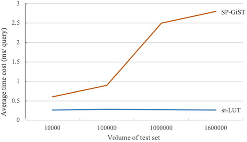
For each query, the spatial search space of the st-LUT indexing method was less than 57,784 scenes (the number of WRS-2 grids) for the worst case scenario. Therefore, the computational times using the SP-GiST and st-LUT were almost the same level when the data size was less than 100,000 scenes. However, when the size of the dataset was greater than 100,000 scenes, the computational time of the SP-GiST increased significantly, while that of the st-LUT remained at a constant level.

5. Discussion

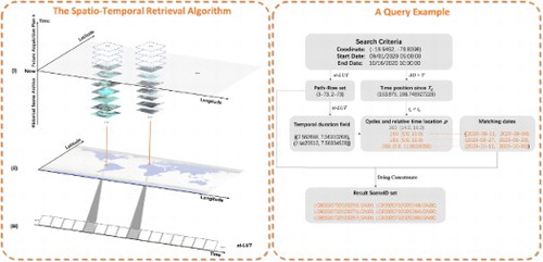
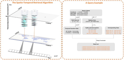
The major contribution of the proposed algorithm is the compression of the search space. By building the st-LUT, the search space is compressed to a constant level. Figure 8 illustrates the compression of the search space and gives a query example. For Landsat 8, the original archive contains more than 1,700,000 scenes from 2013. A query such as searching scenes taken from UTC time 09/01/2020 05:00:00–10/16/2020 10:00:00 at location (−18.6462, −70.8398) would do spatial operations among all the historical scenes. In addition, when new scenes are added, it is necessary to update the spatial index. However, the proposed spatio-temporal indexing model, i.e. the st-LUT, has the ability to convert the spatial information between Path-Row numbers and coordinates. The st-LUT compresses the spatial search space from all scenes to one revisiting cycle (from (i) to (ii) in Figure 8). By integrating the spatial and temporal information, it further compresses the grid to a one-dimension table. From (i) to (iii) in Figure 8, it simplifies the index from three dimensions to a one-dimensional look-up table.

Figure 8. Schematic of the proposed spatio-temporal retrieval algorithm and a query example. (left) The proposed algorithm compresses the search space from a varied volume to a one-dimensional table; and (right) a query example.

The proposed st-LUT gives the corresponding relationship between a scene’s location and its revisiting time at the second level. Although a buffer is set as the time window, it still has time query capabilities accurate to the second. Because RSSO satellite imagery follows a regular acquisition rule, our method can predict the spatio-temporal information of future image acquisitions. A quick response to future acquisition prediction helps accelerate satellite scheduling in emergency situations such as earthquakes, forest fires, and searches for missing ships and aircraft. To make future-acquisition predictions, the only extra step is to set n to a larger number in Equation (3) in order to extend the time sequence to a future time.

More generally, this method is good for RSSO satellites because they have a regular reference grid system and a periodic revisiting characteristic. Using this algorithm for other satellites just consists of five steps: building the one-dimensional grid sequence in time order, grouping the historical images according to the grid sequence, analyzing the spatio-temporal pattern of the historical images in each grid unit, building the st-LUT spatial–temporal integrated index, and finally realizing spatio-temporal query algorithms. The structure of the st-LUT is decided by the organization of the native reference grid systems employed by individual satellite systems. For example, Landsat 8 uses WRS-2, and Sentinel-2′s tiling grid is based on the Military Grid Reference System (MGRS). Regardless of the type of reference grid system used, the revisiting feature is always applicable for these RSSO satellites.

For the existing large-scale remote sensing data catalogue like the Global Earth Observation System of Systems (GEOSS), the aforementioned algorithm can be applied on the basis of the existing metadata service. Once the st-LUT is established for the remote sensing images, the space–time retrieval algorithm could be established and then deployed to substitute the current search capability. Ideally, the method described in this article can achieve better performance than the traditional method to search images on the whole dataset.

Furthermore, the method is only suitable for satellites that have a regular grid system. For satellites like SAR and InSAR that are capable of acquiring images on-demand, since the spatio-temporal coverages of the resultant images do not exhibit a revisiting pattern, the algorithm presented in this paper does not work. Actually, according to WMO’s database, Landsat, CBERS, Sentinel-2 and totally 451 Earth observation satellites are RSSO ones.

6. Conclusions

In this paper, a spatial–temporal data retrieval method for RSSO satellite imagery was proposed. RSSO satellite image data are very commonly used for Earth observation purposes. The proposed method takes advantage of the revisiting feature of RSSO satellites to build a spatio-temporal look-up table using one revisiting cycle. A search algorithm was developed based on this characteristic. Three query scenarios were implemented to explain the algorithm. More than 1,850,000 Landsat 8 scenes were used as an example. The proposed method is different from the traditional space–time indexing methods in that the indexing will not change as new data are added. By using the Landsat 8 image metadata archive as a case study, we compared the results of the proposed method with those of other spatio-temporal indexing and querying methods and found that the efficiency of the proposed method is not affected by the volume of the data.

This image data retrieval method compresses the search space to a constant-level and improves the search efficiency. Based on the st-LUT, it realizes an optimization for large-volume RSSO historical image data retrieval. Compared with other current and heavily used indexing models, the space of our index remains constant and will not change as the data volume increases. In addition, the proposed method is also suitable for other RSSO satellites. Its improvement in terms of the search complexity will help to reduce maintenance costs and increase image query speeds.

Another advantage of this method is its ability to quickly predict a future image acquisition situations. It can provide users with the ability to query when satellites acquire data over their area of interest and to query the acquisition location at any given time. This will help to evaluate the satellite observation coverage.

There are still several limitations to the proposed method. One is that the proposed solution cannot ensure that the st-LUT covers all of the possible revisiting times, especially for future situations, leading to a recall rate of less than 100%. Furthermore, the method is only suitable for satellites that have a regular grid system. Therefore, satellites such as SAR and InSAR that are able to acquire images on-demand, so their spatio-temporal coverages of resultant images do not follow the pattern utilized in this spatio-temporal integrated algorithm.

Disclosure statement

No potential conflict of interest was reported by the author(s).

Correction Statement

This article has been republished with minor changes. These changes do not impact the academic content of the article.

Additional information

Funding

This work was supported by National Key Research and Development Program of China: [grant number 2019YFE0126400].

References

- Arce, Gonzalo R, Jan Bacca, and José L Paredes. 2009. “Nonlinear Filtering for Image Analysis and Enhancement.” In The Essential Guide to Image Processing, edited by Alan C Bovik, 263–291. Orlando, U.S: Academic Press.
- Bai, Yuqi, and Liping Di. 2011. “Providing Access to Satellite Imagery Through OGC Catalog Service Interfaces in Support of the Global Earth Observation System of Systems.” Computers & Geosciences 37 (4): 435–443.
- Bai, Yuqi, Liping Di, Aijun Chen, Yang Liu, and Yaxing Wei. 2007. “Towards a Geospatial Catalogue Federation Service.” Photogrammetric Engineering & Remote Sensing 73 (6): 699–708.
- Bai, Yuqi, Liping Di, Douglas D Nebert, Aijun Chen, Yaxing Wei, Xuanang Cheng, Yuanzheng Shao, Dayong Shen, Ranjay Shrestha, and Huilin Wang. 2012. “GEOSS Component and Service Registry: Design, Implementation and Lessons Learned.” IEEE Journal of Selected Topics in Applied Earth Observations and Remote Sensing 5 (6): 1678–1686.
- Baumann, Peter, Paolo Mazzetti, Joachim Ungar, Roberto Barbera, Damiano Barboni, Alan Beccati, Lorenzo Bigagli, Enrico Boldrini, Riccardo Bruno, and Antonio Calanducci. 2016. “Big Data Analytics for Earth Sciences: the EarthServer Approach.” International Journal of Digital Earth 9 (1): 3–29.
- Bayer, Rudolf, and Edward McCreight. 2002. “Organization and Maintenance of Large Ordered Indexes.” In Software Pioneers, edited by Manfred Broy and Ernst Denert, 245–262. New York City, US: Springer.
- Beckmann, N., H. P. Kriegel, and B. Seeger. 1990. “The R*-Tree: an Efficient and Robust Method for Points and Rectangles.” Proceedings of the 1990 ACM SIGMOD conference.
- Carvalho, Alexandre, Cristina Ribeiro, and A. Augusto Sousa. 2006. “A Spatio-Temporal Database System Based on Timedb and Oracle Spatial.” In Research and Practical Issues of Enterprise Information Systems, edited by A Min Tjoa, Li Da Xu, Maria Raffai, and Niina Maarit Novak, 11–20. New York City, US: Springer.
- Cf, O. D. D. S. 2015. “Transforming our world: the 2030 Agenda for Sustainable Development”.
- Chang, Fay, Jeffrey Dean, Sanjay Ghemawat, Wilson C Hsieh, Deborah A Wallach, Mike Burrows, Tushar Chandra, Andrew Fikes, and Robert E Gruber. 2008. “Bigtable: A Distributed Storage System for Structured Data.” ACM Transactions on Computer Systems (TOCS) 26 (2): 1–26.
- The Charter. 2021. “The International Charter Space and Major Disasters.” Accessed March 6 2021. https://disasterscharter.org/web/guest/home.
- Cordova, Aaron, Billie Rinaldi, and Michael Wall. 2015. Accumulo: Application Development, Table Design, and Best Practices. Sebastopol, US: O'Reilly Media, Inc.
- Finkel, Raphael A., and Jon Louis Bentley. 1974. “Quad Trees a Data Structure for Retrieval on Composite Keys.” Acta Informatica 4 (1): 1–9.
- Fox, Anthony, Chris Eichelberger, James Hughes, and Skylar Lyon. 2013. “Spatio-temporal Indexing in Non-Relational Distributed Databases.” 2013 IEEE International Conference on Big data.
- Gargantini, Irene. 1982. “An Effective Way to Represent Quadtrees.” Communications of the ACM 25 (12): 905–910.
- Kamel, Ibrahim, and Christos Faloutsos. 1993. Hilbert R-tree: An improved R-tree Using Fractals.
- Klinger, Allen, and Charles R Dyer. 1976. “Experiments on Picture Representation Using Regular Decomposition.” Computer Graphics and Image Processing 5 (1): 68–105.
- Li, Jian, and David P Roy. 2017. “A Global Analysis of Sentinel-2A, Sentinel-2B and Landsat-8 Data Revisit Intervals and Implications for Terrestrial Monitoring.” Remote Sensing 9 (9): 902.
- Mahmood, Nadeem, Syed Muhammad Aqil Burney, Kashif Rizwan, Asadullah Shah, and Adnan Nadeem. 2017. “Building Spatio-temporal Database Model Based on Ontological Approach Using Relational Database Environment.”
- Manolopoulos, Yannis, Alexandros Nanopoulos, Apostolos N Papadopoulos, and Yannis Theodoridis. 2010. R-trees: Theory and Applications. Berlin, Germany: Springer Science & Business Media.
- NASA. 2020. “The Worldwide Reference System.” Accessed 2020-11-10. https://landsat.gsfc.nasa.gov/the-worldwide-reference-system/.
- Nascimento, Mario A., and Jefferson R. O. Silva. 1998. “Towards Historical R-trees.” ACM Symposium on Applied Computing.
- Oscar, W. M. O. 2019. OSCAR Observing Systems Capability Analysis and Review Tool.
- Samet, Hanan. 1990. The Design and Analysis of Spatial Data Structures. Vol. 85. Reading, MA: Addison-Wesley.
- Sellis, Timos, Nick Roussopoulos, and Christos Faloutsos. 1987. The R+-Tree: A Dynamic Index for Multi-Dimensional Objects.
- Tao, Yufei, Dimitris Papadias, and Jimeng Sun. 2003. “The TPR*-Tree: an Optimized Spatio-Temporal Access Method for Predictive Queries.” International Conference on very large data bases.
- UN. 2015. Transforming Our World: The 2030 Agenda for Sustainable Development. New York City, US: UN General Assembly.
- Wertz, James Richard. 2001. “Mission Geometry: Orbit and Constellation Design and Management: Spacecraft Orbit and Attitude Systems.” Mission Geometry: Orbit and Constellation Design and Management: Spacecraft Orbit and Attitude Systems/James R. Wertz. El Segundo, CA; Boston: Microcosm: Kluwer Academic Publishers, 2001. Space technology library; 13.
- Wilkinson, Mark D, Michel Dumontier, IJsbrand Jan Aalbersberg, Gabrielle Appleton, Myles Axton, Arie Baak, Niklas Blomberg, Jan-Willem Boiten, Luiz Bonino da Silva Santos, and Philip E Bourne. 2016. “The FAIR Guiding Principles for Scientific Data Management and Stewardship.” Scientific Data 3 (1): 1–9.
- Wulder, Michael A, Joanne C White, Thomas R Loveland, Curtis E Woodcock, Alan S Belward, Warren B Cohen, Eugene A Fosnight, Jerad Shaw, Jeffrey G Masek, and David P Roy. 2016. “The Global Landsat Archive: Status, Consolidation, and Direction.” Remote Sensing of Environment 185: 271–283.
- Yang, Jun, Peng Gong, Rong Fu, Minghua Zhang, Jingming Chen, Shunlin Liang, Bing Xu, Jiancheng Shi, and Robert Dickinson. 2013. “The Role of Satellite Remote Sensing in Climate Change Studies.” Nature Climate Change 3 (10): 875–883.
- Zhang, H. K., and David P. Roy. 2016a. “Landsat 5 Thematic Mapper Reflectance and NDVI 27-Year Time Series Inconsistencies due to Satellite Orbit Change.” Remote Sensing of Environment 186: 217–233. %@ 0034-4257.
- Zhang, H. K., and David P. Roy. 2016b. “Landsat 5 Thematic Mapper Reflectance and NDVI 27-Year Time Series Inconsistencies due to Satellite Orbit Change.” Remote Sensing of Environment 186: 217–233.
- Zhao, Lei, Peiquan Jin, Lanlan Zhang, Huaishuai Wang, and Sheng Lin. 2011. “Developing an Oracle-Based Spatio-Temporal Information Management System.” International Conference on database Systems for advanced applications.
- Zhu, Qing, Jun Gong, and Yeting Zhang. 2007. “An Efficient 3D R-Tree Spatial Index Method for Virtual Geographic Environments.” Isprs Journal of Photogrammetry & Remote Sensing 62 (3): 217–224.
- Zhu, Xiaolin, Eileen H Helmer, Feng Gao, Desheng Liu, Jin Chen, and Michael A Lefsky. 2016. “A Flexible Spatiotemporal Method for Fusing Satellite Images with Different Resolutions.” Remote Sensing of Environment 172: 165–177.