Improving the estimation of canopy cover from UAV-LiDAR data using a pit-free CHM-based method

ABSTRACT

Accurate and rapid estimation of canopy cover (CC) is crucial for many ecological and environmental models and for forest management. Unmanned aerial vehicle-light detecting and ranging (UAV-LiDAR) systems represent a promising tool for CC estimation due to their high mobility, low cost, and high point density. However, the CC values from UAV-LiDAR point clouds may be underestimated due to the presence of large quantities of within-crown gaps. To alleviate the negative effects of within-crown gaps, we proposed a pit-free CHM-based method for estimating CC, in which a cloth simulation method was used to fill the within-crown gaps. To evaluate the effect of CC values and within-crown gap proportions on the proposed method, the performance of the proposed method was tested on 18 samples with different CC values (40−70%) and 6 samples with different within-crown gap proportions (10−60%). The results showed that the CC accuracy of the proposed method was higher than that of the method without filling within-crown gaps (R² = 0.99 vs 0.98; RMSE = 1.49% vs 2.2%). The proposed method was insensitive to within-crown gap proportions, although the CC accuracy decreased slightly with the increase in within-crown gap proportions.

KEYWORDS:

• Canopy cover
• light detecting and ranging
• unmanned aerial vehicle
• within-crown gaps
• pit-free CHM

1. Introduction

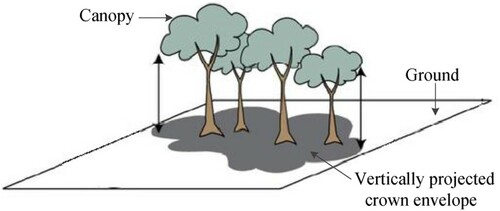
Canopy cover (CC) is defined as the fraction of ground covered by the vertically projected crown envelope (Jennings, Brown, and Sheil 1999; Rautiainen, Stenberg, and Nilson 2005; Gschwantner et al. 2009). Specifically, the definition regards the cover as a solid object; that is, within-crown gaps are included, as shown in Figure 1 (Jennings, Brown, and Sheil 1999; Rautiainen, Stenberg, and Nilson 2005; Gschwantner et al. 2009; Ma, Su, and Guo 2017; Tang et al. 2019; Li et al. 2020). CC plays a key role in the assessment of forest floor microclimate and light conditions (Hansen et al. 2013; Mu et al. 2018), wildlife habitat modeling (Smart et al. 2012) and timber volume estimation (Jennings, Brown, and Sheil 1999). Rapid and accurate estimation of CC is urgently needed to improve the accuracy and applicability of these models (Li et al. 2015; Wu et al. 2019).

Figure 1. Schematic illustration of canopy cover (Dyer et al. 2014). Canopy cover is the fraction of ground covered by the vertically projected crown envelope (gray area), which is considered solid.

Conventionally, CC is assessed through field measurements with tools such as Cajanus tubes and line intersect sampling (Korhonen et al. 2006; Korhonen et al. 2011; Ma, Su, and Guo 2017; Wu et al. 2019). Ground-based data collection is highly time-consuming, laborious and expensive; thus, it can only be used to obtain the CC over a small area and may not be usable in certain forested areas due to the lack of access (Ma, Su, and Guo 2017). Optical remote sensing features have the advantages of acquiring CC data rapidly at a large scale. Numerous efforts have been devoted to two-dimensional image-measured CC (Carreiras, Pereira, and Pereira 2005; Ozdemir 2008; Ko et al. 2009; Pekin and Macfarlane 2009; Karlson et al. 2015; Parmehr et al. 2016; Korhonen et al. 2017; Li et al. 2018). However, the overall estimation accuracy may be unreliable since the radiometric information from these images is seriously impacted by the light and shadow conditions in a forest (Asner 2003; Tang et al. 2019). For example, parts of tree crowns are often shadowed by neighboring canopies and are difficult to identify as canopy from the images, causing CC underestimation (Ma, Su, and Guo 2017).

Light detection and ranging (LiDAR), an active remote sensing technique, has become a reliable tool for forest inventories given its capability to provide precise three-dimensional structural information of forests (Hyyppä et al. 2008; Liang et al. 2016; Zhang et al. 2019; Shao et al. 2020). Moreover, LiDAR data are independent of solar illumination and shadow effects (Cao et al. 2012; Wulder et al. 2012; Zhu et al. 2018). The airborne LiDAR system, one of the most frequently used LiDAR platforms, has been used to estimate CC in various forest types (Smith et al. 2009; Korhonen et al. 2011; Ma, Su, and Guo 2017; Tang et al. 2019). Ma, Su, and Guo (2017), Korhonen, Heiskanen, and Korpela (2013), and Li et al. (2015) demonstrated that LiDAR was superior to passive optical imagery in CC estimation, and CC estimation from airborne LiDAR can be a promising alternative to ground truthing. The CHM-based method is widely used to estimate CC from LiDAR point clouds due to its advantage of being independent from off-nadir scan angles. Specifically, some pulses transmitted at large scan angles may yield uneven sampling of the measured area, causing bias in CC estimation. Uniform sampling is generated by CHM data, and then the CC is estimated by calculating the ratio between the number of canopy pixels and the total number of pixels (Holmgren, Nilsson, and Olsson 2003; Korhonen et al. 2006; Hopkinson 2007; Ma, Su, and Guo 2017; Tang et al. 2019; Wu et al. 2019).

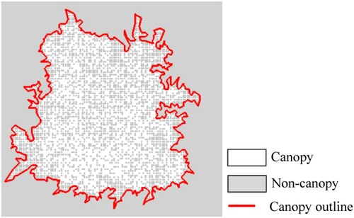
In recent years, as a low-altitude airborne LiDAR system, the use of unmanned aerial vehicle-light detecting and ranging (UAV-LiDAR) systems has gradually increased in forest investigations, especially in applications emphasizing crown shape, due to their higher mobility, lower cost, and higher point density than platforms at high altitudes (Jaakkola et al. 2010; Lin, Hyyppä, and Jaakkola 2011; Wallace et al. 2012; Liu et al. 2018; Cao et al. 2019; Liang et al. 2019). In addition, compared with platforms at high altitudes, the UAV-LiDAR system can transmit narrower laser beams and, therefore, is more likely to penetrate the canopy through within-crown gaps and even reach non-canopy components (such as the understory vegetation or the ground). In CHMs, within-crown gaps appear as pits, whose heights are significantly lower than those of their neighbors. The forest canopy extracted from CHMs using a height threshold (typically set to 2 m) has many holes rather than being a solid object. Therefore, the vertically projected area of the canopy is underestimated, resulting in CC underestimation. As shown in Figure 2, large quantities of within-crown gaps are classified as non-canopy at a height threshold of 2 m, leading to approximately 50% CC underestimation.

Figure 2. A sample of the effect of within-crown gaps on CC estimation. The CC was underestimated by approximately 50%, as many within-crown gaps were classified as non-canopy (i.e. gray pixels within the red outline). Note that reference canopy pixels were located in the canopy outlines that were manually delineated, and the reference CC was calculated as a ratio of the number of reference canopy pixels to the total pixels.

This study aims to improve CC estimation from UAV-LiDAR point clouds by suppressing the influence of within-crown gaps. To address this objective, we used the cloth simulation method to construct a pit-free CHM in which within-crown gaps were filled. The pit-free CHM was used to estimate CC by calculating the fraction of canopy pixels. To validate the proposed method, 18 samples with different CC values (40−70%) were used to assess CC accuracy. In addition, the performance of the proposed method was further assessed on 6 samples with different proportions of within-crown gaps (10−60%).

2. Materials and methods

2.1. Real data

2.1.1. Study area

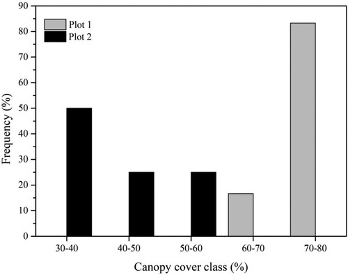
This study was conducted in the Saihanba National Forest Park, Chengde, Hebei province (${42}^{\circ }23.87^{\mathrm{\prime }}\mathrm{N},{117}^{\circ }19.05^{\mathrm{\prime }}\mathrm{E}$). The area is characterized by a subhumid continental climate with an annual average temperature of −1.4°C and an average annual precipitation of approximately 450 mm. The elevation ranges from 1100 m to 1940m. The forest covers more than 70,000 ha and is dominated by planted conifer forests and natural broadleaf forests. The main conifer and broadleaf tree species are Larix principis-rupprechtii and Betula platyphylla, respectively. A conifer forest site and a broadleaf forest site were established to evaluate the performance of the proposed method, which were named as Plots 1 and 2. The terrain of Plots 1 and 2 features flat and sloped, respectively. Each of the two sites was divided into 12 samples that were 25 m × 25 m in size. Six samples in Plot 1 were discarded since these samples contain roads, which are represented by black crosses in Figure 3. CC values of all 18 samples in Plots 1 and 2 range from 40% to 70%, and the distribution of their CC levels is shown in Figure 4.

Figure 3. Location of the study area. Two of the UAV-LiDAR data acquisition sites (named as Plots 1 and 2) and corresponding forest types. Each of the two sites was divided into 12 samples, in which six samples containing roads are discarded (marked by black crosses).

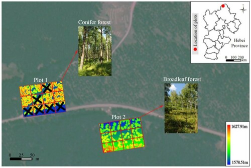
Figure 4. Distribution of canopy cover levels of Plots 1 and 2.

2.1.2. UAV-LiDAR data collection

In this study, the SZT-R250 LiDAR system (ZHENGTU LIDAR, Beijing, China) was used to collect UAV-LiDAR point clouds. This system consists of two main parts: a four-rotor UAV platform and a ground control system. A Rigel mini-1vux LiDAR scanner (RIEGL, Horn, Lower Austria, Austria), a Novatel STIM300 IMU (Novatel, Calgary, Alberta, Canada) and a GNSS (device model is not specified by the manufacturer) were mounted on this UAV platform. The ground control system includes twoterminal devices: one was used to collect LiDAR data, and the other was used to continuously track the aircraft and monitor the UAV flying parameters. Additionally, a South Galaxy G1 GNSS (South, Guangzhou, China) ground base station, with a positioning accuracy of 8 mm + 1 ppm, was used to provide accurate reference measurements and other parameters for postprocessing of the UAV-LiDAR data.

The raw UAV-LiDAR data were collected from 22−23 August 2019, over the research site. The UAV-LiDAR system operated 50 m above ground level, and footprint was 80 mm × 25 mm. In Plots 1 and 2, point density was 271.14 pts/m² and 254.22 pts/m², and the mean point spacing in the horizontal direction was both 0.06 m. The UAV flying parameters and the scanner properties are listed in Table 1.

Table 1. Flight parameters and scanner properties of the UAV-LiDAR data acquisition.

Parameters of four-rotor UAV	Value
Fight altitude (m)	50
Flight velocity (m/s)	5
Swath width (m)	40
Wavelength (nm)	Near Infrared
Beam divergence (mrad)	1.6 × 0.5
Footprint (mm)	80 × 25
Scanning angle	±90°
Pulse repetition frequency (kHz)	100
Point density (pts/m^2)	271.14, 254.22

The collected raw LiDAR data were processed as follows. First, the flight trajectories were reconstructed using the processed GNSS and IMU data. Second, the UAV-LiDAR data coordinates were translated into the WGS84 coordinate system in consideration of the flight trajectory information. Finally, all detected points were converted from WGS84 coordinates to UTM Cartesian coordinates.

2.1.3. Establishment of reference data

To evaluate the performance of the proposed method, we generated the reference data of each sample. First, noise points were removed using the elevation frequency histogram of point clouds (Zhang and Lin 2013; Nie et al. 2017). Three parameters needed to be set: the elevation bin size (w), the highest elevation threshold (h) and the lowest elevation threshold (l). For Plot 1, the values of w, h and l were set at 0.02, 1604.45 and 1578.51 m, respectively, and the corresponding values for Plot 2 were 0.02, 1627.91 and 1584.25 m, respectiely. The errors that failed to be automatically removed were manually corrected. Second, ground and nonground points were classified using a cloth simulation filter (CSF) (Zhang et al. 2016). Three main parameters should be set to implement the CSF, that is, the cloth resolution, classification threshold and max iterations, which were set to 0.2 m, 0.1 m and 50, respectively, in Plots 1 and 2. The errors that failed to be automatically classified were manually corrected. A digital terrain model (DTM) was generated using the ground data through standard linear interpolation (Zhang et al. 2020). Third, the normalized point clouds were generated using the DTM. Then, the normalized point clouds were gridded and only the highest point in each grid was retained. Based on the gridded point clouds, CHMs were constructed by standard linear interpolation (Zhang et al. 2020). In Plots 1 and 2, the grid size was set at 0.07 m, which was slightly larger than their mean point spacing. Fourth, in the top view mode, the canopy outlines were manually delineated, and all pixels surrounded by canopy outlines were marked as a canopy. Finally, the CC was calculated as a ratio of the number of canopy pixels to the total pixels in the sample plot. Although the reference data were not classified 100% correctly in terms of practicality, misclassification was much less common in these reference data than in the automatic canopy and non-canopy classification results. Therefore, we assumed that the reference data provided a correct classification of canopy and non-canopy parts in this study.

2.2 Simulated data

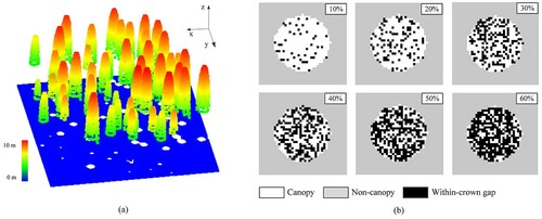
Simulated point cloud data were used to quantify the influence of the number of within-crown gaps on the CC derived from the pit-free CHM-based method. Six semiellipsoid canopy scenes with different proportions of within-crown gaps (10−60%) were generated. The semiellipsoid model is expressed as z$=\sqrt{r^2-64x^2-64y^2},(x^2+y^2\le r^2,z>0)$, where $(x,y,z)$ are the simulated point coordinates and r is the base radius. The within-crown gaps were randomly created in canopies, and their heights were randomly reduced from their original elevations. It was implemented with the C++ programming language. Figure 5 shows a canopy scene and individual canopies with different proportions of within-crown gaps. With the increase in within-crown gap proportions, individual within-crown gaps were gradually merged into within-crown gap clusters, which had various sizes and irregular shape. The point space of the simulated scene data was 0.05 m. The ground and canopy point heights were 0 m and greater than 2 m, respectively.

Figure 5. Simulated point cloud data. (a) Canopy scene. (b) Samples of individual canopies with different proportions of within-crown gaps (10−60%).

2.3. Estimation of canopy cover using pit-free CHM

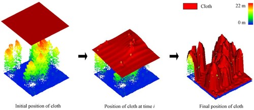
When using the CHM-based method to estimate the CC, the within-crown gaps in CHM, which had smaller values than the canopy height threshold of 2 m, would be classified as non-canopy, leading to CC underestimation. To overcome this problem, we proposed a pit-free CHM-based method to estimate CC. The within-crown gaps in a CHM would be filled in a pit-free CHM. A pit-free CHM construction method based on cloth simulation was used in this study because of the following merits: (a) it is capable of filling within-crown gaps of various sizes; (b) it does not change the values of all CHM pixels while filling the within-crown gaps; and (c) it only requires a CHM resolution parameter to be established. The experiments using the cloth simulation-based method mentioned above were significantly better than those constructed using the mean and median filtered methods, as evidenced by the lowest average root mean square error (cloth simulation-based method: 0.5 m; mean filtered method: 1.16 m; median filtered method: 1.01 m). This method involves the simulation of the physical process of a cloth touching an object (Figure 6). A simulated cloth is iteratively dropped onto a height-normalized forest point cloud; the simulated cloth sticks to the uppermost layer of the forest canopy and bridges over the within-crown gaps due to the degree of hardness of the simulated cloth. A more detailed description of this method is given in the literature (Zhang et al. 2020). In the present study, the pit-free CHMs in Plots 1 and 2 were generated with a resolution of 0.07 m, which was slightly larger than their mean point spacing because this size was not only able to characterize the tree crown as finely as possible but also reduce the data redundancy in each pixel (Zhao et al. 2013). Based on the pit-free CHMs, the CC was estimated using Equation (1): (1) $\mathrm{C}\mathrm{C}=\frac{\sum \mathrm{C}\mathrm{H}{\mathrm{M}}_{\mathrm{c}\mathrm{a}\mathrm{n}\mathrm{o}\mathrm{p}\mathrm{y}}}{\sum \mathrm{C}\mathrm{H}{\mathrm{M}}_{\mathrm{t}\mathrm{o}\mathrm{t}\mathrm{a}\mathrm{l}}}$(1) where $\mathrm{C}\mathrm{H}{\mathrm{M}}_{\mathrm{c}\mathrm{a}\mathrm{n}\mathrm{o}\mathrm{p}\mathrm{y}}$ is the pixels of the pit-free CHM belonging to the canopy (with a CHM value above 2 m). $\mathrm{C}\mathrm{H}{\mathrm{M}}_{\mathrm{t}\mathrm{o}\mathrm{t}\mathrm{a}\mathrm{l}}$ is the total number of pit-free CHM pixels.

Figure 6. Overview of the cloth simulation method.

2.4. Accuracy assessment

The accuracy of CC estimation was evaluated by using the coefficient of determination (R²) and root mean squared error (RMSE), which were calculated as follows (Ma, Su, and Guo 2017): (2) $R^2=1-\frac{{\sum }_{i=1}^n{(\mathrm{C}{\mathrm{C}}_i-{\widehat{\mathrm{C}\mathrm{C}}}_i)}^2}{{\sum }_{i=1}^n{(\mathrm{C}{\mathrm{C}}_i-\overline{\mathrm{C}\mathrm{C}})}^2}$(2) (3) $\mathrm{R}\mathrm{M}\mathrm{S}\mathrm{E}=\sqrt{\sum _{i=1}^n{(\mathrm{C}{\mathrm{C}}_i-{\widehat{\mathrm{C}\mathrm{C}}}_i)}^2/n}$(3)

where n is the number of samples; $\mathrm{C}{\mathrm{C}}_i$ and ${\widehat{\mathrm{C}\mathrm{C}}}_i$ represent the reference and estimated results at the ith sample, respectively; and $\overline{\mathrm{C}\mathrm{C}}$ is the mean of all reference data.

The error of the CC estimates of each sample achieved using the CHM and pit-free CHM-based methods was evaluated using two indicators, that is, the underestimation and overestimation errors. The underestimation error is the ratio of the number of misclassified canopy pixels to the total number of pixels, whereas the overestimation error is the ratio of the number of misclassified non-canopy pixels to the total number of pixels. The formulas for the underestimation and overestimation errors are expressed as follows: (4) $\mathrm{u}\mathrm{n}\mathrm{d}\mathrm{e}\mathrm{r}\mathrm{e}\mathrm{s}\mathrm{t}\mathrm{i}\mathrm{m}\mathrm{a}\mathrm{t}\mathrm{i}\mathrm{o}\mathrm{n}\mathrm{e}\mathrm{r}\mathrm{r}\mathrm{o}\mathrm{r}=\mathrm{a}/\mathrm{c}$(4) (5) $\mathrm{o}\mathrm{v}\mathrm{e}\mathrm{r}\mathrm{e}\mathrm{s}\mathrm{t}\mathrm{i}\mathrm{m}\mathrm{a}\mathrm{t}\mathrm{i}\mathrm{o}\mathrm{n}\mathrm{e}\mathrm{r}\mathrm{r}\mathrm{o}\mathrm{r}=\mathrm{b}/\mathrm{c}$(5) where a is the number of canopy pixels misclassified as non-canopy pixels, b is the number of non-canopy pixels misclassified as canopy pixels, and c is the total number of pixels.

3. Results

3.1. Evaluation of real data

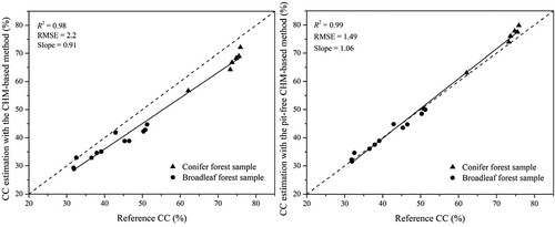
Figure 7 shows the relationship between the reference and estimated CC for the 18 samples. The CC values derived from the pit-free CHM-based method had better agreement with the reference dataset (R² = 0.99 vs 0.98) and higher precision (RMSE = 1.49% vs 2.2%) than the CHM-based method across various CC levels.

Figure 7. Canopy cover estimations with the (a) CHM and (b) pit-free CHM-based methods for all samples. The dashed line denotes a 1:1 relationship, and the solid line is the fitted line.

Table 2 presents the underestimation and overestimation errors for the CHM and pit-free CHM-based methods on Plots 1 and 2. On average, the underestimation error of the pit-free CHM-based method was only one-fifth of that of the CHM-based method. With respect to the overestimation error, the difference in accuracy between the different methods was slight, with an average of 0.45%.

Table 2. Underestimation and overestimation errors of the CHM and pit-free CHM-based methods.

	CHM-based method (%)			Pit-free CHM-based method (%)
	Underestimation error	Overestimation error		Underestimation error	Overestimation error
Plot 1	9.24	2.9		1.07	3.22
Plot 2	8.01	3.5		2.66	2.28
Average	8.63	3.2		1.87	2.75

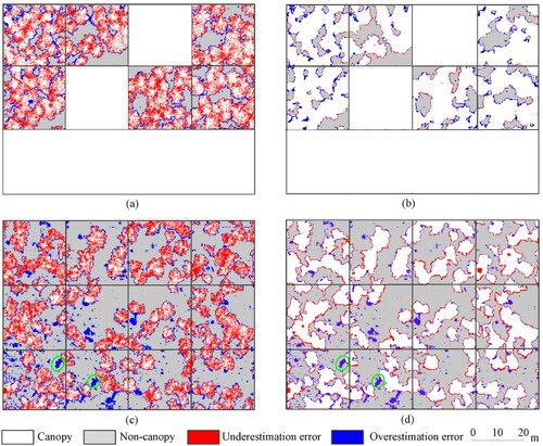
Figure 8 shows the distributions of the underestimation and overestimation errors of the CHM and pit-free CHM-based methods on Plots 1 and 2. It is clear that the underestimation error of the CHM-based method was mainly located in the region covered by a vertical projection of the tree crown, as shown in Figure 8(a,c). The underestimation error of the CHM-based method was effectively removed by the pit-free CHM-based method. The distributions of the overestimation error of the two methods were similar, and they tended to be located in understory vegetation. In addition, parts of inclined trunks were incorrectly accepted as the canopy, such as those denoted by the green circles in Figure 8(c,d).

Figure 8. Error distributions of the (the first column) CHM and (the second column) pit-free CHM-based methods in Plots 1 and 2. (a) and (b) are Plot 1; (c) and (d) are Plot 2. In (a) and (b), blank rectangular regions are the discarded samples since they contain roads. In (c) and (d), regions inside the green circle represent the overestimation error caused by the inclined trunk.

3.2. Evaluation of simulated data

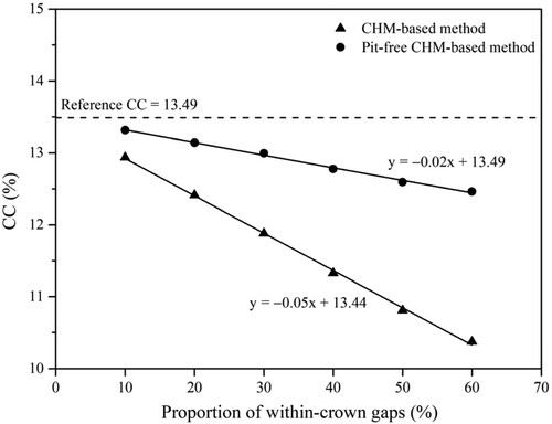
Figure 9 shows the CC estimation accuracy of the CHM and pit-free CHM-based methods under different proportions of within-crown gaps (10−60%), in which the reference CC is 13.49%. From 10% to 60% within-crown gaps, the CC values estimated by the CHM method decreased from 12.94% to 10.38%, while CC values estimated by the pit-free CHM-based method decreased from 13.32% to 12.46%. Overall, with the increase in within-crown gaps, the CC estimation accuracy of the pit-free CHM-based method deteriorated. However, the decay rate of the pit-free CHM-based method was much lower than that of the CHM-based method (slope = −0.02 vs −0.05).

Figure 9. Influences of proportion of within-crown gaps (from 10% to 60%, with an interval of 10%) on the CC estimation accuracies for the CHM and pit-free CHM-based methods.

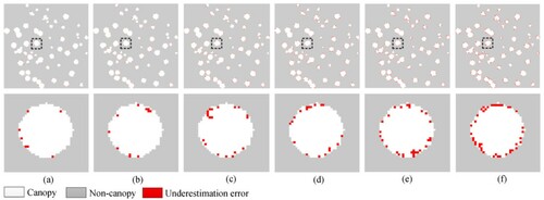
As shown in Figures 10 and 11, only underestimation error was present for the CHM and pit-free CHM-based methods on simulated data. The pit-free CHM-based method removed most of the underestimation errors, although a small number of errors were present at the edge of tree crowns (Figure 11). Moreover, the underestimation error increased with the increase in within-crown gap proportions.

Figure 10. Error distribution of the CHM-based method at different proportions of within-crown gaps: (a) 10%, (b) 20%, (c) 30%, (d) 40%, (e) 50%, and (f) 60%. The region framed by the dashed rectangle is magnified on the underside.

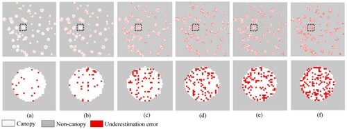
Figure 11. Error distribution of the pit-free CHM-based method at different proportions of within-crown gaps: (a) 10%, (b) 20%, (c) 30%, (d) 40%, (e) 50%, and (f) 60%. The region framed by the dashed rectangle is magnified on the underside.

4 Discussion

4.1. Analysis of errors

4.1.1. Underestimation error

CHM construction is an important prerequisite for estimating CC. However, large quantities of within-crown gaps in a CHM may cause obvious CC underestimation. In this study, a pit-free CHM-based method was proposed to improve CC estimation, which constructed a CHM without within-crown gaps and then estimated CC based on the CHM. The results showed that the underestimation error caused by within-crown gaps was one key reason why the estimation of CC using UAV-LiDAR point clouds is biased and imprecise (Table 2 and Figure 8). This finding aligns with those obtained from several other data sources, such as full-waveform airborne LiDAR data and ultrafine-resolution images (Korhonen et al. 2006; Tang et al. 2019). Therefore, it is necessary to reduce the underestimation error caused by within-crown gaps to improve the CC estimation accuracy of UAV-LiDAR point clouds.

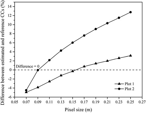
The CHM-based method can reduce the CC underestimation error by setting a high pixel size. Specifically, after setting a high pixel size, each within-crown gap point is not generated to an individual pixel but a mixed pixel with multiple points. In the mixed pixel, within-crown gap points (i.e. low points inside the canopy) are usually neglected because only the highest point is retained. The example shown in Figure 12 demonstrates that within-crown gaps are gradually neglected with increasing pixel size. Meanwhile, tree crown edges are gradually blurred due to the expansion of tree crown edges (Figure 13), which also increases CC estimation value. Both of the above factors (neglect of within-crown gaps and expansion of tree crown edges) contribute to the increase in CC estimation value. However, how to set the optimal pixel size for accurate CC estimation in different areas is still challenging since the optimal parameter may be related to multiple factors, such as the number of within-crown gaps and the length of the tree crown edges (Jennings, Brown, and Sheil 1999; Ma, Su, and Guo 2017). Based on the reference CC, we identified the optimal pixel size of Plots 1 and 2 by a trial-and-error process. It can be found that their optimal pixel sizes were 0.15 and 0.09 m, and CC estimation results were sensitive to the pixel size since a small change in the pixel size may lead to a large change in the difference between the estimated and reference CCs, as shown in Figure 14. In comparison, the proposed method used raw pixel size (i.e. slightly larger than mean point spacing) to alleviate the negative effects of within-crown gaps in CC estimation. Result showed that the CC estimation results of the proposed method were quite close to the reference CCs (R² = 0.99, RMSE = 1.49%) due to the significant reduction in CC underestimation error (Figures 7 and 8). It proved the effectiveness of the proposed method for alleviating the negative effects of within-crown gaps.

Figure 12. Canopy covers derived from different pixel sizes. (a) 0.07 m, (b) 0.13 m, (c) 0.21 m, and (d) 0.25 m.

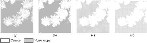
Figure 13. A sample with reference canopy sampling points overlaid on the CHM.

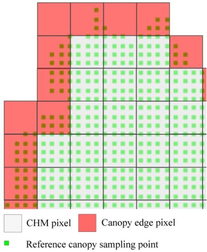
Figure 14. The sensitivity of the CHM-based method to the setting of pixel size.

4.1.2. Overestimation error

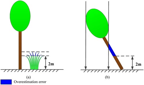
For the CHM and pit-free CHM-based methods, the overestimation error was mainly distributed on understory vegetation (Figure 8). This result may be explained by the fact that the tree crown and understory vegetation cannot be accurately distinguished based on a height threshold of 2 m (Figure 15(a)). Such errors can be reduced by setting a higher threshold, such as the 5 m height criteria in the forest definition of the Food and Agriculture Organization of the United Nations, but it will increase the risk of tree crown pixels being misclassified as understory vegetation. Devising methods for better separating tree crowns and understory vegetation presents a challenge for CC estimation that needs to be addressed in future studies. In addition, parts of inclined trunks were misclassified as tree crowns, as shown in the green circles in Figure 8(c,d). This phenomenon can be explained by the fact that the inclined trunks cannot be hidden in the vertical projection of the tree crown (Figure 15(b)). In the inclined and vertical states, the vertical projection area of the tree crown was inconsistent. However, this situation had not yet been considered in the definition of CC. Thus, a refined definition will be needed considering that high-resolution remote sensing data, such as UAV-LiDAR data, provide great potential for identifying area differences between the two states.

Figure 15. The distributions of overestimation error. (a) Understory vegetation. (b) Inclined trunk.

4.2. The impact of within-crown gap proportions on the proposed method

This study investigated the effects of different proportions of within-crown gaps on the proposed method. The results showed that the CC estimation accuracy of the pit-free CHM-based method had a weak negative correlation with proportions of within-crown gaps. Moreover, all errors were located at the edge of tree crowns. This effect occurred because the proportions of within-crown gaps were positively correlated with the number of within-crown gaps at the edge of tree crowns. Moreover, the proposed method failed to fill the within-crown gaps at the edge of tree crowns. Thus, the larger the proportion of within-crown gaps, the lower the CC estimation accuracy of the pit-free CHM-based method. To further improve the CC estimation accuracy of the proposed method, we will continue to improve the filling of within-crown gaps at the edge of tree crowns in future studies.

5. Conclusion

This study was conducted to develop a more accurate method for estimating CC from UAV-LiDAR point clouds by suppressing the influence of within-crown gaps. A pit-free CHM-based method was proposed to estimate CC. The proposed method used cloth simulation to fill the within-crown gaps. We demonstrated the effectiveness of the proposed method by conducting a comparison with the CHM-based method. The CHM and pit-free CHM-based methods were evaluated on 24 samples with various CC values and within-crown gap proportions. The results showed that the presence of large quantities of within-crown gaps was a key factor leading to biased estimation of CC. Compared with the CHM-based method, the pit-free CHM-based method obtained higher accuracy due to the limitation of underestimation error caused by within-crown gaps. Taken together, these findings highlight the necessity of alleviating the negative effects of within-crown gaps to obtain accurate CC estimations from UAV-LiDAR point clouds, and the pit-free CHM-based method demonstrated the potential for the improvement of CC estimation.

Disclosure statement

No potential conflict of interest was reported by the author(s).

Additional information

Funding

This work was supported by the National Natural Science Foundation of China (grant numbers 41971380 and 41671414), Guangxi Natural Science Fund for Innovation Research Team (grant number 2019JJF50001), and the Open Fund of State Key Laboratory of Remote Sensing Science (grant number OFSLRSS201920).

References

- Asner, Gregory P., and Amanda S. 2003. “Canopy Shadow in IKONOS Satellite Observations of Tropical Forests and Savannas.” Remote Sensing of Environment 87 (4): 521–533.
- Cao, Chunxiang, Yunfei Bao, Min Xu, Wei Chen, Hao Zhang, Qisheng He, Zengyuan Li, et al. 2012. “Retrieval of Forest Canopy Attributes Based on a Geometric-Optical Model Using Airborne LiDAR and Optical Remote-Sensing Data.” International Journal of Remote Sensing 33 (3): 692–709.
- Cao, Lin, Kun Liu, Xin Shen, Xiangqian Wu, and Hao Liu. 2019. “Estimation of Forest Structural Parameters Using UAV-LiDAR Data and a Process-Based Model in Ginkgo Planted Forests.” IEEE Journal of Selected Topics in Applied Earth Observations and Remote Sensing 12 (11): 4175–4190.
- Carreiras, João M.B., José M.C. Pereira, and João S. Pereira. 2005. “Estimation of Tree Canopy Cover in Evergreen Oak Woodlands Using Remote Sensing.” Forest Ecology and Management 223 (1–3): 45–53.
- Dyer, Fiona J., Ben Broadhurst, Ross M. Thompson, Kim Jenkins, Patrick Donald Driver, Neil Saintilan, Sharon Bowen, et al. 2014. “Commonwealth Environmental Water Office Long Term Intervention Monitoring Project. Lachlan River System.” In Commonwealth Environmental Water Office Technical Report, 1–192. Canberra: University of Canberra.
- Gschwantner, Thomas, Klemens Schadauer, Claude Vidal, Adrian Lanz, Erkki Tomppo, Lucio Di Cosmo, Nicolas Robert, et al. 2009. “Common Tree Definitions for National Forest Inventories in Europe.” Silva Fennica 43 (2): 303–321.
- Hansen, M. C., P. V. Potapov, R. Moore, M. Hancher, S. A. Turubanova, A. Tyukavina, D. Thau, et al. 2013. “High-resolution Global Maps of 21st-Century Forest Cover Change.” Science 342: 850–853.
- Holmgren, J., M. Nilsson, and H. Olsson. 2003. “Simulating the Effects of Lidar Scanning Angle for Estimation of Mean Tree Height and Canopy Closure.” Canadian Journal of Remote Sensing 29 (5): 623–632.
- Hopkinson, Chris. 2007. “The Influence of Flying Altitude, Beam Divergence, and Pulse Repetition Frequency on Laser Pulse Return Intensity and Canopy Frequency Distribution.” Canadian Journal of Remote Sensing 33 (4): 312–324.
- Hyyppä, J., H. Hyyppä, D. Leckie, F. Gougeon, X. Yu, and M. Maltamo. 2008. “Review of Methods of Small-Footprint Airborne Laser Scanning for Extracting Forest Inventory Data in Boreal Forests.” International Journal of Remote Sensing 29 (5): 1339–1366.
- Jaakkola, Anttoni, Juha Hyyppä, Antero Kukko, Xiaowei Yu, Harri Kaartinen, Matti Lehtomäki, and Yi Lin. 2010. “A Low-cost Multi-sensoral Mobile Mapping System and Its Feasibility for Tree Measurements.” ISPRS Journal of Photogrammetry and Remote Sensing 65 (6): 514–522.
- Jennings, S. B., N. D. Brown, and D. Sheil. 1999. “Assessing Forest Canopies and Understorey Illumination: Canopy Closure, Canopy Cover and Other Measures.” Forestry 72 (1): 59–74.
- Karlson, Martin, Madelene Ostwald, Heather Reese, Josias Sanou, Boalidioa Tankoano, and Eskil Mattsson. 2015. “Mapping Tree Canopy Cover and Aboveground Biomass in Sudano-Sahelian Woodlands Using Landsat 8 and Random Forest.” Remote Sensing 7 (8): 10017–10041.
- Ko, Dongwook, Nathan Bristow, David Greenwood, and Peter Weisberg. 2009. “Canopy Cover Estimation in Semiarid Woodlands: Comparison of Field-based and Remote Sensing Methods.” Forest Science 55 (2): 132–141.
- Korhonen Lauri, Hadi, Petteri Packalen, and Miina Rautiainen. 2017. “Comparison of Sentinel-2 and Landsat 8 in the Estimation of Boreal Forest Canopy Cover and Leaf Area Index.” Remote Sensing of Environment 195: 259–274.
- Korhonen, Lauri, Janne Heiskanen, and Ilkka Korpela. 2013. “Modelling Lidar-derived Boreal Forest Canopy Cover with SPOT 4 HRVIR Data.” International Journal of Remote Sensing 34 (22): 8172–8181.
- Korhonen, Lauri, Kari T. Korhonen, Miina Rautiainen, and Pauline Stenberg. 2006. “Estimation of Forest Canopy Cover: A Comparison of Field Measurement Techniques.” Silva Fennica 40 (4): 577–588.
- Korhonen, Lauri, Ilkka Korpela, Janne Heiskanen, and Matti Maltamo. 2011. “Airborne Discrete-return LIDAR Data in the Estimation of Vertical Canopy Cover, Angular Canopy Closure and Leaf Area Index.” Remote Sensing of Environment 115 (4): 1065–1080.
- Li, Linyuan, Jun Chen, Xihan Mu, Weihua Li, Guangjian Yan, Donghui Xie, and Wuming Zhang. 2020. “Quantifying Understory and Overstory Vegetation Cover Using UAV-based RGB Imagery in Forest Plantation.” Remote Sensing 12 (2): 1–18.
- Li, Linyuan, Xihan Mu, Craig Macfarlane, Wanjuan Song, Jun Chen, Kai Yan, and Guangjian Yan. 2018. “A Half-Gaussian Fitting Method for Estimating Fractional Vegetation Cover of Corn Crops Using Unmanned Aerial Vehicle Images.” Agricultural and Forest Meteorology 262 (November 2017): 379–390.
- Li, Wang, Zheng Niu, Xinlian Liang, Zengyuan Li, Ni Huang, Shuai Gao, Cheng Wang, and Shakir Muhammad. 2015. “Geostatistical Modeling Using LiDAR-derived Prior Knowledge with SPOT-6 Data to Estimate Temperate Forest Canopy Cover and Above-ground Biomass via Stratified Random Sampling.” International Journal of Applied Earth Observation and Geoinformation 41: 88–98.
- Liang, Xinlian, Ville Kankare, Juha Hyyppä, Yunsheng Wang, Antero Kukko, Henrik Haggrén, Xiaowei Yu, et al. 2016. “Terrestrial Laser Scanning in Forest Inventories.” ISPRS Journal of Photogrammetry and Remote Sensing 115: 63–77.
- Liang, Xinlian, Yunsheng Wang, Jiri Pyörälä, Matti Lehtomäki, Xiaowei Yu, Harri Kaartinen, Antero Kukko, et al. 2019. “Forest In Situ Observations Using Unmanned Aerial Vehicle as an Alternative of Terrestrial Measurements.” Forest Ecosystems 6. Article 20.
- Lin, Yi, Juha Hyyppä, and Anttoni Jaakkola. 2011. “Mini-UAV-borne LIDAR for Fine-scale Mapping.” IEEE Geoscience and Remote Sensing Letters 8 (3): 426–430.
- Liu, Kun, Xin Shen, Lin Cao, Guibin Wang, and Fuliang Cao. 2018. “Estimating Forest Structural Attributes Using UAV-LiDAR Data in Ginkgo Plantations.” ISPRS Journal of Photogrammetry and Remote Sensing 146: 465–482.
- Ma, Qin, Yanjun Su, and Qinghua Guo. 2017. “Comparison of Canopy Cover Estimations from Airborne LiDAR, Aerial Imagery, and Satellite Imagery.” IEEE Journal of Selected Topics in Applied Earth Observations and Remote Sensing 10 (9): 4225–4236.
- Mu, Xihan, Wanjuan Song, Zhan Gao, Tim R. McVicar, Randall J. Donohue, and Guangjian Yan. 2018. “Fractional Vegetation Cover Estimation by Using Multi-angle Vegetation Index.” Remote Sensing of Environment 216: 44–56.
- Nie, Sheng, Cheng Wang, Pinliang Dong, Xiaohuan Xi, Shezhou Luo, and Haiming Qin. 2017. “A Revised Progressive TIN Densification for Filtering Airborne LiDAR Data.” Measurement 104: 70–77.
- Ozdemir, I. 2008. “Estimating Stem Volume by Tree Crown Area and Tree Shadow Area Extracted from Pan-sharpened Quickbird Imagery in Open Crimean Juniper Forests.” International Journal of Remote Sensing 29 (19): 5643–5655.
- Parmehr, Ebadat G., Marco Amati, Elizabeth J. Taylor, and Stephen J. Livesley. 2016. “Estimation of Urban Tree Canopy Cover Using Random Point Sampling and Remote Sensing Methods.” Urban Forestry and Urban Greening 20: 160–171.
- Pekin, Burak, and Craig Macfarlane. 2009. “Measurement of Crown Cover and Leaf Area Index Using Digital Cover Photography and Its Application to Remote Sensing.” Remote Sensing 1 (4): 1298–1320.
- Rautiainen, Miina, Pauline Stenberg, and Tiit Nilson. 2005. “Estimating Canopy Cover in Scots Pine Stands.” Silva Fennica 39 (1): 137–142.
- Shao, Jie, Wuming Zhang, Nicolas Mellado, Nan Wang, Shuangna Jin, Shangshu Cai, Lei Luo, Thibault Lejemble, and Guangjian Yan. 2020. “SLAM-aided Forest Plot Mapping Combining Terrestrial and Mobile Laser Scanning.” ISPRS Journal of Photogrammetry and Remote Sensing 163: 214–230.
- Smart, L. S., J. J. Swenson, N. L. Christensen, and J. O. Sexton. 2012. “Three-dimensional Characterization of Pine Forest Type and Red-cockaded Woodpecker Habitat by Small-footprint, Discrete-return Lidar.” Forest Ecology and Management 281: 100–110.
- Smith, Alistair M.S., Michael J. Falkowski, Andrew T. Hudak, Jeffrey S. Evans, Andrew P. Robinson, and Caiti M. Steele. 2009. “A Cross-comparison of Field, Spectral, and Lidar Estimates of Forest Canopy Cover.” Canadian Journal of Remote Sensing 35 (5): 447–459.
- Tang, Hao, Xiao-Peng Song, Feng A. Zhao, Alan H. Strahler, Crystal L. Schaaf, Scott Goetz, Chengquan Huang, Matthew C. Hansen, and Ralph Dubayah. 2019. “Definition and Measurement of Tree Cover: A Comparative Analysis of Field-, Lidar- and Landsat-based Tree Cover Estimations in the Sierra National Forests, USA.” Agricultural and Forest Meteorology 268: 258–268.
- Wallace, Luke, Arko Lucieer, Christopher Watson, and Darren Turner. 2012. “Development of a UAV-LiDAR System with Application to Forest Inventory.” Remote Sensing 4 (6): 1519–1543.
- Wu, Xiangqian, Xin Shen, Lin Cao, Guibin Wang, and Fuliang Cao. 2019. “Assessment of Individual Tree Detection and Canopy Cover Estimation Using Unmanned Aerial Vehicle Based Light Detection and Ranging (UAV-LiDAR) Data in Planted Forests.” Remote Sensing 11 (8): 908–928.
- Wulder, Michael A., Joanne C. White, Ross F. Nelson, Erik Næsset, Hans Ole Ørka, Nicholas C. Coops, Thomas Hilker, Christopher W. Bater, and Terje Gobakken. 2012. “Lidar Sampling for Large-area Forest Characterization: A Review.” Remote Sensing of Environment 121: 196–209.
- Zhang, Wuming, Shangshu Cai, Xinlian Liang, Jie Shao, Ronghai Hu, Sisi Yu, and Guangjian Yan. 2020. “Cloth Simulation-based Construction of Pit-free Canopy Height Models from Airborne LiDAR Data.” Forest Ecosystems 7. Article 1.
- Zhang, Jixian, and Xiangguo Lin. 2013. “Filtering Airborne LiDAR Data by Embedding Smoothness-constrained Segmentation in Progressive TIN Densification.” ISPRS Journal of Photogrammetry and Remote Sensing 81: 44–59.
- Zhang, Wuming, Jianbo Qi, Peng Wan, Hongtao Wang, Donghui Xie, Xiaoyan Wang, and Guangjian Yan. 2016. “An Easy-to-use Airborne LiDAR Data Filtering Method Based on Cloth Simulation.” Remote Sensing 8 (6): 501–522.
- Zhang, Wuming, Peng Wan, Tiejun Wang, Shangshu Cai, Yiming Chen, Xiuliang Jin, and Guangjian Yan. 2019. “A Novel Approach for the Detection of Standing Tree Stems from Plot-level Terrestrial Laser Scanning Data.” Remote Sensing 11 (2): 211–229.
- Zhao, Dan, Yong Pang, Zengyuan Li, and Guoqing Sun. 2013. “Filling Invalid Values in a Lidar-derived Canopy Height Model with Morphological Crown Control.” International Journal of Remote Sensing 34 (13): 4636–4654.
- Zhu, Xi, Andrew K. Skidmore, Tiejun Wang, Jing Liu, Roshanak Darvishzadeh, Yifang Shi, Joe Premier, and Marco Heurich. 2018. “Improving Leaf Area Index (LAI) Estimation by Correcting for Clumping and Woody Effects Using Terrestrial Laser Scanning.” Agricultural and Forest Meteorology 263: 276–286.