19-year remotely sensed data in the forecast of spectral models of the environment

ABSTRACT

The aims of this study were: i) to compare no-till areas in two municipalities located in different regions of Brazil, along with the influence on CO₂Flux and GPP, and ii) to verify the difference between environmental factors followed by the trends of these variables regarding future scenarios (ARIMA time-series model number). The study was carried out in two areas with different latitudes in the municipalities of Sinop-MT and Passo Fundo-RS, both in Brazil. A time series of 19 years was performed with data acquired by remote sensing from the following satellites: i) Landsat-8 (OLI and TIRS), and ii) TERRA/AQUA (MODIS). The results propound that the spectro-temporal variables are directly influenced by soil management and agricultural practices over the observation time, with a satisfactory correlation in future predictions of the variables for the next ten years, in which presented that the variation of GPP and albedo values for the two study sites would gradually increase until 2028 and the temperature remained constant between the range of its seasonality, and CO₂Flux tends to decrease in its seasonality, indicating a higher CO₂ absorption.

KEYWORDS:

• ARIMA
• numerical modeling
• remote sensing
• orbital products
• tillage

1. Introduction

The growth of the world population has increasingly demanded the conversion of forested areas into agricultural fields. These changes in land use and land occupation, together with the burning of fossil fuels, are the largest emitters of greenhouse gases (GHGs). The increase in GHG emissions and their contribution to global warming has led to the search for mitigation strategies that reduce the sources of these gases (Carvalho et al. 2010; Carvalho et al. 2016) and the search for more sustainable agriculture, which are one of the significant challenges of current society.

Soil tillage interventions are carried out to prepare the arable land for sowing and planting. Such soil changes by intensive cultivation can cause long-term damage and hence lead to soil degradation for crop growth and increase the potential for environmental degradation (Reicosky, Sauer, and Hatfield 2011; Lal 2015). Soybean [Glycine max (L.) Merril] is a crop that has been highlighted in the world scenario due to its use in food and the size of its grown area (Silva Junior et al. 2020). In Brazil, soybean occupied more than 33 million hectares (M/ha) in the 2018/2019 crop year (SOJAMAPS 2020), making the country the second-largest producer in the area, just behind the USA, the first world exporter of this oilseed.

In soybean sowing, tillage techniques (T) are used, which consist of using plowing and harrowing for the incorporation of correctives, fertilizers, plant residues, and weeds, or soil surface decompaction. On the other hand, no-tillage (NT) has become a widespread conservation practice in recent years, as it seeks to keep the soil always covered by developing crops and plant residues. Thus, NT increase the carbon (C) surface in soil, maintain the soil structure and hence reduce soil degradation under intensive agriculture (Didoné et al. 2014; Alliaume et al. 2014; Barut and Celik 2017; Das et al. 2017). It is known that increasing organic C on the surface can improve the soil quality (Wick, Kühne, and Vlek 1998; Dexter et al. 2008; Lal 2016; Duval, Martinez, and Galantini 2020; Ramírez et al. 2020).

Tillage and no-till systems have already been evaluated in sugarcane crops based on the verification of the differences in C emissions by each system. In the sugarcane management system based on geostatistical analysis, the clay content in the soil was the outstanding attribute to explain the CO₂ flow (Tavares et al. 2018). Previous studies are worth mentioning for indicating the potential of sugarcane to capture atmospheric CO₂ and promote C sequestration in the soil (La Scala et al. 2001; Silva-Olaya et al. 2013). It is worth noting that these studies were performed by ‘in situ’ assessments, but they can be carried out by remote sensing (RS) techniques.

The contributions of RS techniques by using Terra/Aqua and Landsat satellites can provide advances in studies aimed at characterizing the dynamics of vegetation cover and C on the land surface. By RS, it is possible to both estimate the loss of CO₂ to the atmosphere (Richey et al. 2002; Novo et al. 2005; Czarnogorska, Samsonov, and White 2016; Crowell et al. 2018; Pastick et al. 2020) and carbon absorption through gross primary production – GPP (Silva Junior et al. 2019a; Rossi et al. 2020), and variables such as albedo and temperature can also help to understand these dynamics.

Several studies in the literature aim to quantify the C stored in vegetation, based on future projections about the climate system (Silva, Lopes, and Azevedo 2005; Braga 2013; Wu et al. 2016; Ouyang et al. 2020). Knowing the changes of these variables to the atmosphere is fundamental in studies aiming at monitoring, comparing, and evaluating the impact regarding the modifications of the soil-plant-atmosphere relationship. The information obtained can be applied in strategies for reducing CO₂ emissions to the atmosphere, mainly as input data in numerical simulations and climate projections (Easterling et al. 2000; Solman, Nunez, and Cabré 2008; Silva and Lambers 2020).

Based on the above, the study used RS techniques to evaluate the tillage and no-tillage management systems for soybean sowing in two Brazilian municipalities at different latitudes, to identify i) what system would contribute to more sustainable agriculture with lower GHG emissions?; ii) Is latitude influenced by CO₂ flow and Gross Primary Production (GPP)?; iii) and to check the difference between environmental factors (Albedo, Temperature, GPP, and CO₂Flux), followed by these variables for the future scenario via numerical modeling.

2. Material and methods

2.1. Study area

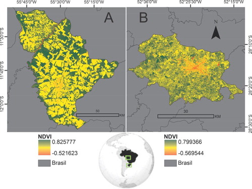
Two study areas were selected: the first is the municipality of Sinop with approximately 3,941.958 km² (IBGE 2020), located in the state of Mato Grosso (MT), Midwest region of Brazil. Sinop is located between 11°20’ to 12°10'S and 55°50’ to 55°10'W, with an altitude of 371 m. According to Köppen classification, the region's climate is ‘Aw’ (hot and humid tropical), with two well-defined seasons: rainy (October to April) and dry (May to September), with average annual rainfall of 1,974.77 mm, respectively, and average monthly temperatures between 23.2 and 25.8°C (Souza et al. 2013) (Figure 1A). The second study area is the municipality of Passo Fundo with approximately 783.603 km² (IBGE 2020), located in the state of Rio Grande do Sul (RS), southern region of Brazil. Passo Fundo is located between 28°6’ to 28°24'S and 52°40’ to 52°12'W, with an attitude of 687 m. According to the Köppen classification, the climate is described as subtropical-humid (‘Cfa’), with an average annual temperature of 17.5°C and above 30°C in summer, and an annual rainfall of 1,787.8 mm (Figure 1B).

Figure 1. Geographical location of Sinop – MT (A) and Passo Fundo – RS (B) and spatial variability of NDVI (product MOD13Q1.V6) of the temporal mean of the Julian days 206 to 258 of the year 2017, respectively.

2.2. Soybean area detection

The soybean crop mapping was performed with the images from the Landsat 5 satellites (Thematic Mapper – TM), Lansat 7 (Enhanced Thematic Mapper Plus – ETM+), Landsat 8 (Operational Land Imager – OLI e Thermal Infrared Sensor – TIRS) and TERRA/AQUA (Moderate-Resolution Imaging Spectroradiometer – MODIS), through the use of spectral bands according to the methodology previously proposed by Silva Junior et al. (2017).

Based on the soybean cultivation calendar in the state of Mato Grosso and Rio Grande do Sul, the Perpendicular Crop Enhancement Index (PCEI) previously developed by Silva Junior et al. (2017) was obtained. At the initial stage of the soybean crop, the reflections recorded by the sensor may interfere with the PCEI values, since the soil will be without cultivation. To avoid this interference, the Perpendicular Vegetation Index (PVI) Equation (1) was applied, and the red and infrared spectral bands were used for ground line regression, as described by Nanni and Demattê (2006). (1) $PVI={\displaystyle \frac{P_{IVP}-a{P}_V-b}{\sqrt{1+a^2}}}$(1)

Wherein: a and b are, respectively, a slope and the intercept of the ground line, P_V and P_IVP is an independent variable.

Through the PVI time series, the Perpendicular Crop Enhancement Index (PCEI) was calculated, which is represented by Equation (2) and summarized in Equation (3), as described by Silva Junior et al. (2017): (2) $\mathrm{PCEI}=g.{\displaystyle \frac{\left(\mathrm{Max}{\displaystyle \frac{{\rho }_{\mathrm{IVP}}-a{\rho }_V-b}{\sqrt{1+a^2}}+S}\right)-\left(\mathrm{Min}{\displaystyle \frac{{\rho }_{\mathrm{IVP}}-a{\rho }_V-b}{\sqrt{1+a^2}}+S}\right)}{\left(\mathrm{Max}{\displaystyle \frac{{\rho }_{\mathrm{IVP}}-a{\rho }_V-b}{\sqrt{1+a^2}}+S}\right)+\left(\mathrm{Min}{\displaystyle \frac{{\rho }_{\mathrm{IVP}}-a{\rho }_V-b}{\sqrt{1+a^2}}+S}\right)}}$(2) (3) $PCEI={\displaystyle \frac{(MaxPVI+S)-(MinPVI+S)}{(MaxPVI+S)+(MinPVI+S)}}$(3) MaxPVI is the maximum value of PVI observed in the period of maximum development of the soybean crop; MinPVI is the minimum value observed in the period of pre-seeding and/or emergency; S is the coefficient of improvement (10²), and g is the gain factor (10²). All values of the time series for automated detection of soybean areas were implemented in JavaScript on the Google Earth Engine platform and validated by Silva Junior et al. (2017), Silva Junior et al. (2020).

2.3. Vegetation index

For this study, six vegetation indices were used: Normalized Difference Vegetation Index (NDVI), Enhanced Vegetation Index 2 (EVI2), Normalized Difference Senescence Index (NDSVI), Soil Adjusted Total Vegetation Index (SATVI), Soil Tillage Index (STI), and Normalized Difference Tillage Index (NDTI) (Table 1). NDVI and EVI2 quantify the presence of photosynthetic pigments in vegetation. For identifying senescent vegetation and the green vegetation density degree, the NDSVI and SATVI indices were used. In the identification of the dry cover fraction and the soil management system over the years, we used the STI and NDTI indices.

Table 1. Vegetation indices used in the study to estimate the soil management, in 2000/2001 and 2017/2018 crop years

Vegetation Index	Equations	References
Normalized Difference Vegetation (NDVI)	$NDVI={\displaystyle \frac{\rho NIR-\rho RED}{\rho NIR+\rho RED}}$	Rouse et al. (1974)
Enhanced Vegetation Index 2 (EVI2)	$EVI2=2.5\ast {\displaystyle \frac{\rho NIR-\rho RED}{\rho NIR+(2.4\ast \rho RED)+1}}$	Jiang et al. (2008)
Normalized Difference Senescence Index (NDSVI)	$NDSVI={\displaystyle \frac{\rho SWIR1-\rho RED}{\rho SWIR1+\rho RED}}$	Qi et al. (2002)
Soil Adjusted Total Vegetation Index (SATVI)	$SATVI={\displaystyle \frac{\rho SWIR1-\rho RED}{\rho SWIR1+\rho RED+L}(1+L)-\left({\displaystyle \frac{\rho SWIR2}{2}}\right)}$	Marsett et al. (2006)
Soil Tillage Index (STI)	$STI={\displaystyle \frac{\rho SWIR1}{\rho SWIR2}}$	Van Deventer et al. (1997)
Normalized Difference Tillage Index (NDTI)	$NDTI={\displaystyle \frac{\rho SWIR1-\rho SWIR2}{\rho SWIR1+\rho SWIR2}}$	Van Deventer et al. (1997)

Wherein: near-infrared wavelength reflectance $(\rho NIR)$; red wavelength reflectance ($\rho RED$); short-infrared wavelength reflectance ($\rho SWIR1$ and $\rho SWIR2$); Constant (related to the slope of the ground line in a characteristic space graph) which is usually defined as 0.5 (L).

2.4. Discriminating soil management by spectral indices, GEOBIA and data mining

The steps to identify the type of soil management before soybean sowing for the two study areas followed the methodology applied in the Landsat 5, 7, and 8 satellites based on the GEOBIA (Geographic Object-Based Image Analysis) technique and data mining (DM) to improve image processing.

Image processing through multiresolution segmentation sought to explore spatial relationships along with their spectral characteristics or more criteria of homogeneity in one or more dimensions of attribute space (Blaschke 2010; Garcia-Pedrero et al. 2015). The computational environment of the eCognition® software was used to interpret the images by the object-oriented classification method (Gao et al. 2019), together with the WEKA® software, which is a set equipped with learning algorithms for data mining and statistical evaluation tasks (Kalmegh 2015).

The proposed steps are shown in the flowchart (Figure 2), followed by the junction of the images with modification in the radiometric resolution, setting of the segmentation factors, segmentation of the images, selection of the objects to generate the training set, data mining, interpretation and evaluation of the decision tree, classification of the multitemporal data using decision implementation, and classification validation.

Figure 2. Flowchart of the main steps of the study, with emphasis on GEOBIA and data mining in computing environments.

The multiresolution segmentation performed in eCognition®, in which the developed objects (polygons) were exposed to the heterogeneity decision, in which the spectral band weights, form factors and compression were adjusted according to the scale parameter. The adjustment of a scale parameter can influence the size of the developed segments (Liu et al. 2018; Jozdani, Johnson, and Chen 2019; Yang et al. 2019).

In multiresolution segmentation, the similarity rule was established from the difference between the attribute of a probable region and the sum of the values between this attribute in the regions that compose it. Furthermore, the heterogeneity of the color attributes is created from an estimated sum of the standard deviations of each band in a specific region and shape, which were adjusted according to the size of the objects, calculated during the segmentation, generating distinct objects (Shang et al. 2019; Vogels et al. 2019).

The object-based approach offered the possibility of evaluating areas by spectral, textual, contextual, and hierarchical characteristics. Objects can be characterized in the spectral information of the objects based on mean values and standard deviations and in textual spectral information based on the gray level co-occurrence matrix (GLCM) proposed by Haralick, Shanmugam, and Dinstein (1973) and later implemented by Definiens (2006).

All spectral bands and indices used received the weight of 0.5 and 1, respectively, with scale 35 in the two study areas for processing at the same time during segmentation, thus ensuring the homogeneity of objects. After the segmentation, the classes assigned when defining each object as Tillage – T, No-tillage A – NT_A and No-tillage B – NT_B were taken into account (Rossi et al. 2020).

For classifying the objects as T, NT_A, and NT_B in the soybean seeding areas, the decision tree discriminated by Rossi et al. (2020) was implemented in the attributes extracted from the spectral bands and vegetation indices of the two study areas. The decision tree was acquired using the J48 algorithm, which is a C4.5 implementation that chooses an attribute to divide the data into two subsets based on the most significant gain of standardized information (entropy difference).

The advantages of the decision tree classification model are easy to understand and identify them with precision comparable to other classification models (Cruz and Tumibay 2019).

2.5. Land surface temperature (LST)

In this study, an algorithm based on the Landsat satellite series was used to acquire the LST of the study areas, as described by Du et al. (2015). The method is based on the study of atmospheric water vapor inversion based on thermal infrared data from the Landsat satellite to obtain the parameters of atmospheric water vapor (Ren et al. 2015).

The algorithm is based on data from the two thermal infrared channels of the Landsat sensor, Equation (4) of the non-linear two-channel split window. (4) $T_s=B_0+\left(B_2{\displaystyle \frac{1-\epsilon }{\epsilon }+B_3{\displaystyle \frac{{\mathrm{\Delta }}_{\epsilon }}{{\epsilon }^2}}}\right){\displaystyle \frac{T_i+T_j}{2}+\left(B_4+B_5{\displaystyle \frac{1-\epsilon }{\epsilon }+B_6{\displaystyle \frac{{\mathrm{\Delta }}_{\epsilon }}{{\epsilon }^2}}}\right){\displaystyle \frac{T_i+T_j}{2}+B_7(T_i+T_j{)}^2}}$(4) wherein, $\epsilon$ and ${\mathrm{\Delta }}_{\epsilon }$ are the average and the difference in the emissivity of the two channels, respectively, depending on the land cover and cover density; $T_i$ and $T_j$ are the observed radiation brightness of the two channels; B_i is the coefficient whose value can be obtained from experimental data, data from atmospheric parameters, or from simulated atmospheric radiative transfer equation, which depends on the atmospheric water vapor content to improve accuracy.

For reducing the coupling of atmospheric parameters, the algorithm estimates atmospheric water vapor based on thermal infrared data. An empirical relationship is established between the atmospheric transmittance rate $T_i/T_j$ and the atmospheric water vapor (WV) content of the two channels using the atmospheric profiles Moderate Resolution Atmospheric Transmission (MODTRAN) and Thermodynamic Initial Guess Retrieval (TIGR) firstly, and then using the covariance rate and covariance between the brightness temperatures of the two channels in a moving window of a specific size to estimate the atmospheric transmittance rate Equations (5) and (6). (5) $wv=a+b\left({\displaystyle \frac{T_i}{T_j}}\right)+c{\left({\displaystyle \frac{T_i}{T_j}}\right)}^2$(5) (6) ${\displaystyle \frac{T_i}{T_j}\approx R_{ji}={\displaystyle \frac{{\sum }_{k=1}^N(T_{i,k}-{\overline{T}}_j)(T_{i,k}-{\overline{T}}_j)}{{(T_{i,k}-{\overline{T}}_j)}^2}}}$(6)

In Equation (7), the results of the surface temperature calculation without unit were divided by 100 to obtain degrees Kelvin (K) and then converted to Celsius (°C). (7) $LST=T_s-273.15$(7)

2.6. CO₂ flux

For monitoring the described land uses and their carbon losses, it was applied via the TM, RTM+, and OLI sensor systems of the Landsat 5, 7, and 8 satellites, respectively. For this purpose, the orbital images corrected for reflectance factor and the composition mosaic of better tiles by Google Earth Engine platform between 01-01-2000 and 12-31-2018 were used.

The CO₂Flux index (Rahman et al. 2001) was used to measure the in C sequestration efficiency by vegetation, i.e. the photosynthesis rate in the photosynthesis process. For this purpose, the Photochemical Reflectance Index – PRI (Equation 8) was calculated (Gamon, Serrano, and Surfus 1997). For the formulation of this index, the green and blue spectral bands were used. The PRI estimates the leaf carotenoid pigments. These pigments, in turn, indicate the rate of CO₂ storage in leaves (Rahman et al. 2001; Barnes et al. 2017). (8) $PRI={\displaystyle \frac{B-G}{B+G}}$(8) B = Blue spectral band reflectance;

G = Green spectral band reflectance.

However, PRI results need to be rescheduled, resulting in positive values. For this, it is necessary to generate the sPRI Equation (9) (Martins and Baptista 2013). (9) $sPRI={\displaystyle \frac{(PRI+1)}{2}}$(9) Thus, the CO₂Flux index (µmol.m⁻².s⁻¹) was the result of the multiplication between NDVI and sPRI, in which there is a relationship between the PRI index, which indicates the light use efficiency in photosynthesis, and the NDVI, which demonstrates the vigor of photosynthestically active vegetation, in which it can be able to capture absorptions from carbon sequestration (Rahman et al. 2001).

For adequacy of CO₂Flux results with the study site, a correlation of values acquired by remote sensing and values measured by micrometeorological towers was made. The measurements obtained by the towers are determined using the Eddy Covariance method.

According to Boas Dos Santos (2017), the best correlation was through the Equation (10). (10) $CO2FLUX=13.63-(66.207\ast (NDVI\ast sPRI))$(10)

2.7. GPP (Gross primary productivity)

The product MOD17A2 related to gross primary production is a cumulative compound of GPP values based on the concept of solar radiation use efficiency by vegetation (ϵ). In this logic, the primary production is linearly related to absorbed photosynthetic active radiation (APAR), according to the Equation (11). APAR can be calculated as the product of the incident photosynthetically active radiation (PAR), in the visible spectral range from 0.4 μm to 0.7 μm, assumed to be 45% of the total incident solar radiation and the fraction of absorbed photosynthetically active radiation by the vegetation cover (FPAR) (Heinsch et al. 2003; Delgado et al. 2018). (11) $GPP=\epsilon \ast \mathrm{PAR}\ast \mathrm{FPAR}$(11)

One of the most significant challenges in the use of such models is to obtain the light use efficiency ‘ϵ’ in a large area, due to its dependence on environmental factors and vegetation itself. One of the solutions is to relate ‘ϵ’ according to its maximum value (ϵ_max), plus environmental contributions synthesized by minimum air temperature (Tminscalar) and water status in vegetation (VPDscalar – water vapor pressure deficit) (Field, Randerson, and Malmström 1995), according to Equation (12). (12) $\epsilon ={\epsilon }_{max}\ast T_{minscalar}\ast VP{D}_{scalar}$(12) In this study, MODIS GPP (Gross Primary Productivity), version 5.0, with composition on the Google Earth Engine platform, was used between 06-01-2017 and 05-31-2018. The pixel values referring to the digital numbers of the MODIS images were converted into biophysical values (Kg.C. m⁻²) by multiplying by the scale factor (0.0001) (Heinsch et al. 2003) Equation (13) GPP values were also transformed from the accumulated value every eight days to average values every eight days and converted from Kg.C.m⁻².day⁻¹ to g.C.m⁻².day⁻¹. (13) $GPP\mathrm{\_}1\mathrm{Km}={\displaystyle \frac{\mathrm{Biophysical}\mathrm{Pixel}(\mathrm{Kg}\mathrm{C}{\mathrm{m}}^{-2})}{8}}$(13)

2.8. Albedo and radiation balance

According to Allen et al. (2002), albedo is based on the linear integration of the wavelength reflectance with a variation from visible to near and medium infrared, with measurements of the reflectance factor at the top of the atmosphere. For Tasumi et al. (2008), the albedo estimation was created to improve the accuracy of several surface conditions in the energy balance, such as the use and conversion of the land surface mainly by anthropic actions. The albedo is calculated by integrating the surface reflectance of shortwave spectral bands. The surface reflectance factor is derived from orbital images using atmospheric transmittance functions in each spectral band, where atmospheric pressure, solar zenith angle, viewing angle of image acquisition, and calibrated coefficients for different sensors are used (He et al. 2018; Wang et al. 2016).

The surface albedo was calculated in the shortwave radiation domain (0.3 - 3.0 µm), but without atmospheric correction, where it was obtained by a linear combination of spectral reflectances ρ_λ,b, with weights ϖ_λ,b established for each band, as described in Equation (14): (14) ${\alpha }_{toa}=(\varpi {}_2^{}\ast {\rho }_{\lambda ,2})+(\varpi {}_3^{}\ast {\rho }_{\lambda ,3})+(\varpi {}_4^{}\ast {\rho }_{\lambda ,4})+(\varpi {}_5^{}\ast {\rho }_{\lambda ,5})+(\varpi {}_6^{}\ast {\rho }_{\lambda ,6})+(\varpi {}_7^{}\ast {\rho }_{\lambda ,7})$(14)

Thus, each weight was obtained by the ratio between the specific solar constant of band b and the sum of all constants ESUN_λ,b, according to Equation (15): (15) ${\varpi }_{\lambda ,b}={\displaystyle \frac{ENS{U}_{\lambda ,b}}{\mathrm{\Sigma }ENS{U}_{\lambda ,b}}}$(15) Where the values for OLI/LANDSAT-8 are shown in Table 2.

Table 2. Weight Coefficients ($\varpi$n) for the calculation of the planetary albedo through the use of LANDSAT-8 images.

Bands	Band 2	Band 3	Band 4	Band 5	Band 6	Band 7
$\varpi$n	0.300	0.277	0.233	0.143	0.036	0.012
ESUNλ,b	2011.3	1853	1532.8	956.4	237.8	80.2

Source: Silva et al. (2016) adapted by the authors.

Afterward, the albedo was corrected and calculated according to Equation (16), proposed by Tasumi et al. (2008): (16) ${\alpha }_{SUP}={\displaystyle \frac{{\alpha }_{TOA}-{\alpha }_{atm}}{{\tau }_{SW}^2}}$(16) wherein: α_atm is the portion of solar radiation reflected by the atmosphere, adopted as 0.03, according to Bastiaanssen (2000), in which $\tau$_SW is the atmospheric transmittance for bright sky days in Equation (17), proposed by Allen et al. (2002): (17) ${\tau }_{SW}=0.75+2\ast {10}^{-5}\ast DEM$(17) wherein: DEM is the digital elevation model, represented by the altitude (m) of each pixel, which was used by the mission with the Shuttle Radar Topography Mission (SRTM).

After obtaining the LAI values, the Surface Emissivity (ϵ₀) was calculated using the inverted Plank equation, proposed for a black body. The calculation of ϵ₀ is performed based on the LAI, according to (18) ${\epsilon }_0=0.95+0.01\ast LAI$(18)

For calculating the LST, the monochromatic radiance was previously computed based on the band 10 of the Thermal Infrared Sensor (TIRS) LANDSAT-8, using the radiance rescaling factors provided in the metadata (USGS 2019) Equation (19): (19) $L_{\lambda }=M_L{Q}_{cal}+A_L$(19) wherein: L_λ is the monochromatic radiance, M_L is the specific multiplicative rescaling factor (3.342 × 10⁻⁴), A_L is the specific additive rescaling factor (0.1), and Q_cal is the pixel-to-pixel value of the orbital image, using the Equation (20): (20) $Ts={\displaystyle \frac{K_2}{\ln ((K_1/K_2)+1)}}$(20) where: K₂ and K₁ are thermal band 10 calibration constants.

Then the emitted long-wave radiation W m⁻²) for each pixel was calculated (by Stefan-Boltzmann's Equation (21), as a function of temperature Ts and surface emissivity ϵ₀: (21) $R_{ol,emi}={\epsilon }_0.\sigma .T_s^4$(21) wherein σ is the Boltzmann constant (5.67*10⁻⁸ W m⁻² K⁻⁴).

The incident longwave radiation (W.m⁻²) was also calculated according to Stefan-Boltzmann's Equation Equation (22), as a function of the air emissivity (ϵ_a) and air temperature (T_a, obtained by the surface station), given by: (22) $R_{ol,atm}={\epsilon }_0.\sigma .T_a^4$(22) where: (22) ${\epsilon }_a=0.85\ast (-\ln {\tau }_{SW}{)}^{0.09}$(22) The incident shortwave radiation (W.m⁻²) was considered constant for the study area, and given the lack of pyranometric data, it was obtained according to the model below (Allen et al. 2002; Gomes 2009) Equation (23): (23) $Rs=Q.\cos \theta .dr.{\tau }_{SW}$(23) wherein $Q$ is the solar constant (1367 W m⁻²); θ is the solar incidence angle; $dr$ is the distance Earth-Sun, and ${\tau }_{sw}$ is the atmospheric transmissivity (calculated according to Equation (24)).

The radiation balance – Rn (W.m⁻²) was obtained according to Equation (24): (24) $Rn=(1-\alpha ).R_S+R_{ol,atm}-R_{ol,emi}-(1-{\epsilon }_0).R_{ol,atm}$(24) wherein: α is the surface albedo; $R_s$ incident shortwave radiation; $R_{\mathrm{ol},\mathrm{atm}}$ is the incident long-wave radiation; $R_{\mathrm{ol},\mathrm{emi}}$ emitted long-wave radiation, and ${\epsilon }_0$ is the surface emissivity (4–100 µm).

2.9. ARIMA – Future and past modeling

The Autoregressive Integrated Moving Average Model (ARIMA) was used to predict likely changes in the following variables: CO₂Flux, Albedo, GPP, and Temperature from the data series of the study area on the soy mask. ARIMA models have two general forms (p, d, and q) and (P, D, Q), non-seasonal and seasonal, respectively, according to Equation (25). The seasonal model was used in this study, in which AR(p) refers to the number of observations of delay included in the model, also called the order of delay in the regression equation for the series Y. I (d) refers to the number of times in which gross observations are differentiated, also called degree of differentiation, and MA (q) is the term for the moving average, leading to the observation of previous errors. The data of the analyzed variables were parameterized following their values of minimum and maximum variation for each author. (25) $Y_t=c+{\mathrm{\varnothing }}_1{y}_{d}t-1+{\mathrm{\varnothing }}_p{y}_{d}t-p+\dots +{\mathrm{\varnothing }}_1{e}_{t-1}+{\mathrm{\varnothing }}_q{e}_{t-q}+e_t$(25) wherein, y (d) is Y differentiated d times, and c are constants, p is the autoregressive order, d is the differentiation order (1 or 2 usually), and q is the moving average order.

The validation occurred by generating the 8-year data series, i. e., from the model, the previous series of 132 samples were generated to predict the next year. All years considered were validated from the following statistical indicators: Standard Error of the Estimate (SEE), coefficient of determination (R²), and Willmott's concordance index (d). The future simulation of the variables CO₂Flux, Albedo, GPP, and Temperature was performed for ten years, from January 2019 to December 2028, using monthly data from the 19-year time series (2000 to 2018). These models depend directly on past values and, therefore, they operate well on long and stable series (Valipour 2015).

All processing was performed in R software version 3.5.1 using the libraries (MASS, tseries, forecast, readxl, raster, rgdal, maptools, RSAGA, and ggplot2) (R CORE TEAM 2015).

3. Results and discussion

3.1. Identifying soybean in the study areas by MODIS

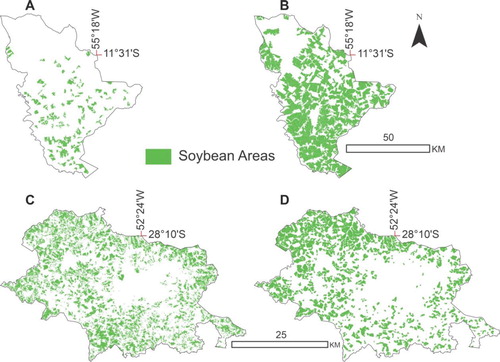
Soybean detection in Sinop – MT and Passo Fundo – RS, for 2000/2001 and 2017/2018 crop years by MODIS sensor, is shown in Figure 3. In 2000/2001, 34,875.95 ha (Sinop, MT) and 22,461.58 ha (Passo Fundo, RS) were mapped, respectively. In 2017/2018, the mapped area was 199.519,97 ha (Sinop, MT) and 21.886,41 ha (Passo Fundo, RS). Comparatively, there was a considerable increase of 472% and a decrease of 2.56%. This increase in cultivated area between the crop years is due to the increase in international demand and attractive soybean prices, which hence contributed to a significant increase in cultivated areas in the municipality of Sinop (CONAB 2019).

Figure 3. Mapping of soybean (ha) in 2000/2001 (A and C) and 2017/2018 (B and D) crop years in the municipalities of Sinop -MT (A and B) and Passo Fundo-RS (C and D) by MODIS sensor.

The findings obtained by mapping were satisfactory in the discrimination of soybean cultivation areas. Other studies, such as Gusso et al. (2013), Spera et al. (2016), Kastens et al. (2017), Silva Junior and Lima (2018), and Silva Junior et al. (2019b) also corroborate the efficiency of the methodology used in this study.

3.2. Vegetation indices

Figure 4 shows the vegetation indices in the municipalities of Sinop-MT and Passo Fundo-RS. The vegetation indices showed high spatial variability among the municipalities, mainly in the 2017/2018 crop year (Figure 4), in which the highest production and soybean growing area was verified (SOJAMAPS 2020; CONAB 2019; IBGE 2020). Passo Fundo-RS showed a higher amount of areas with vegetative density compared to Sinop-MT, according to EVI2 and NDVI. It is worth mentioning that cultivation areas in the state of RS are common to use forage crops, before soybean sowing and, however, the state of MT does not have this habit among farmers (Alvarenga et al. 2001; Carvalho et al. 2013).

Figure 4. Vegetation indices for the 2017/2018 crop year in the municipalities of Passo Fundo-RS (A) and Sinop-MT (B).

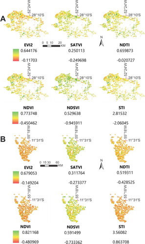
The NDTI and STI indices, in Passo Fundo-RS, pointed to the greater agglomeration of areas with dry cover fraction to the soil management system in relation to Sinop-MT, as already demonstrated in previous studies (Dai et al. 2018; Chai et al. 2019; Wang et al. 2019). Highlight to the SATVI and NDSVI indices that presented almost proportional senescence of vegetation between the two municipalities.

It is worth noting that the values obtained from EVI2 and NDVI, concerning the spectral behavior of the soil, can be affected by several factors. For example, due to the presence of moisture, organic matter content, presence of iron oxide (Fe₂O₃), the proportion of clay, silt, sand and the roughness of the soil, which in turn interfere in the electromagnetic energy with the soil (Moraes Novo 2010; Ponzoni, Shimabukuro, and Kuplich 2012; Gholizadeh et al. 2018).

The multispectral images and vegetation indices were extracted as close as possible to the beginning of the soil preparation for soybean sowing so that the spectral bands would not suffer extreme interference with humidity (CONAB 2019; Yue et al. 2019).

3.3. GEOBIA and classification of soil management

Figure 5 shows the efficiency of applying multiresolution segmentation in the spectral bands and the vegetation indices. The segmentation presented in Figure 5 (A) showed distinct discrimination of the generated objects (polygons), visually perceived when applying the combination of false color (RGB) on the image. Other studies have reported a higher precision when using the classification by multiresolution segmentation (Blaschke 2010; Kavzoglu and Tonbul 2017; Yin et al. 2017; Wang et al. 2020). With acceptable discrimination of objects in both study areas, the automated decision tree classification method (Rossi et al. 2020) was used, which can discriminate in Figure 5 (B) the types of soil management (T, NT_A, and NT_B).

Figure 5. Segmentation and application of the decision tree in the municipalities of Passo Fundo-RS (A1/B1) and Sinop-MT (A2/B2) in the 2000/2001 and 2017/2018 crop years.

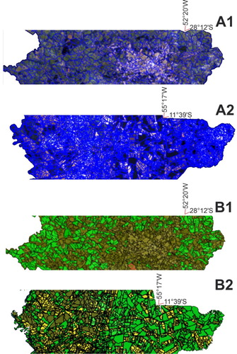
The image segmentation technique presented an acceptable object variation for applying the decision tree algorithm. It is worth noting that previous studies used a similar segmentation methodology to analyze changes in land cover and land use (Souza-Filho et al. 2018; Xi et al. 2019), detection of central pivot irrigated areas (Vogels et al. 2019), and weed discrimination (LÓPEZ-GRANADOS 2011; De Castro, López-Granados, and Jurado-Expósito 2013; Castillejo-González et al. 2014).

Figure 6 represents the discrimination of the thematic map of the studied areas regarding the types of soybean cultivation after the application of the decision tree algorithm. The results obtained indicate a higher intensity of soil management for no-till B in Passo Fundo-RS, in all crop year analyzed. On the other hand, Sinop-MT presented a variation in the soil management system, since, in the previous crop years (2000/2001), the T had the highest domain and later, in the 2017/2018, there was higher soil management by NT_B, with a significant increase for the NT_A if compared to the previous crop year. This fact is due to the arrival time of soybean cultivation in each municipality and its large-scale production. For example, the implementation of soybean in Passo Fundo began before 2000, and the intensification in production occurred from 2005. On the other hand, soybean areas in Sinop were minimal in 2000, and its intensification in production began in 2010 (IBGE 2020).

Figure 6. Discrimination of the areas studied regarding the type of soil management in 2000/2001 and 2017/2018 crop years. A – Passo Fundo and B – Sinop-MT.

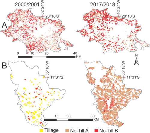
Comparatively, Passo Fundo-RS in the 2000/2001 crop year compared to Sinop-MT presented a higher percentage (86.14%) of the area prepared with the NT_A (Table 3). This finding is justified by the amount of planted area in each municipality, as described in item 3.1. However, in the 2017/2018 crop year, Sinop-MT exceeded Passo Fundo-RS in 91.43% of the area identified as NT_A. In the NT_B occurred the same, since in 2000/2001 Passo Fundo-RS presented areas with NT_B 40.74% greater than Sinop-MT, but in 2017/2018, there was a significant change in which Sinop-MT presented an area 77.69% greater (Table 3).

Table 3. Total area (ha) using tillage (T), no-till A (NT_A), and no-till B (NT_B) in the 2000/2001 and 2017/2018 crop years in the municipalities of Passo Fundo-RS and Sinop-MT.

Municipality	Crop Year	T (ha)	NT_A (ha)	NT_B (ha)
Passo Fundo	2000/2001	0	853.65	13,921.93
	2017/2018	0	14,063.01	7,823.39
Sinop	2000/2001	26,507.55	118.31	8,250.07
	2017/2018	383.70	164,066.52	35,069.74

The boxplot exploratory analysis represented by the time series in 19 years of study for albedo, CO₂FLUX, GPP, and temperature are shown in Figure 7. The albedo calculated for Passo Fundo-RS for NT_A was 0.15. The highlights were September 2010 (0.283), with the highest average albedo, and August 2016 (0.061) with lower value, respectively. Regarding the NT_B, the average albedo was 0.19, where the highest emission occurred in August 2017 (0.462) and the smallest in August 2015 (0.058). For no-till management systems, the largest albedo was recorded for NT_B. However, both systems coincided with the lowest albedo production, recorded in August in subsequent years.

Figure 7. Boxplot of annual values of albedo, CO₂Flux, GPP, and Temperature for time series 2000 to 2018 in the two municipalities studied.

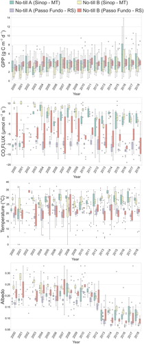
In Sinop-MT, the albedo average emitted during the analyzed years was for NT_A (0.18) and NT_B (0.21). The months with the highest albedo values were October 2010 (0.36) and January 2001 (0.516) for NT_A and NT_B, respectively. The minimum values were obtained in August 2015 (0.07) and June 2013 (0.10) (NT_A and NT_B). The municipalities of Passo Fundo and Sinop are related to the lower production of albedo for NT_A and higher for NT_B.

The amount of emission (-) and absorption (+) of CO₂Flux can be verified in Figure 7. The months of highest CO₂Flux emissions for NT_A occurred in August 2016 (Passo Fundo-RS) and December 2012 (Sinop-MT) – (Figure 7). For NT_B, the months with the highest CO₂Flux emissions were February 2016 (Passo Fundo-RS) and March 2013 (Sinop-MT), respectively. It is worth mentioning that the municipalities of Passo Fundo and Sinop absorbed practically the same amount of CO₂Flux in the NT_B over the entire time series. However, in 2017, Passo Fundo absorbed less CO₂Flux.

GPP values showed a distinct peak in each municipality from 2000 to 2011. Peaks were high in early November to the end of February for NT_A and NT_B in Passo Fundo-RS (Figure 7). In Sinop-MT, peaks occurred from early February to the end of June. However, from 2012 until 2018, the GPP peaks of the two municipalities start together from November until the end of March. The average temperature for NT_A varied from 20.64 °C for Passo Fundo to 26.20 °C for Sinop. In NT_B, these temperatures were around 21.20 °C to 27.16 °C for Passo Fundo and Sinop. Therefore, the temperatures in Sinop are higher than Passo Fundo over the entire 19-year time series.

The comparison of environmental variables at different latitudes, as shown in Figure 7, does not characterize the differentiation between T and NT. For, in Passo Fundo – RS, there was no discrimination of areas with T at the beginning of the time series. We decided to compare the environmental variables in Sinop-MT, which showed areas with NT in its time series (Figure 8).

Figure 8. Boxplot of annual values of Albedo, CO₂Flux, GPP, and Temperature for time series 2000 to 2018 in the municipality of Sinop – MT.

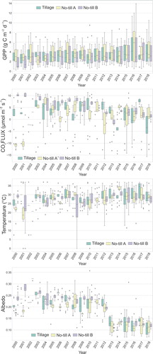
Average temperature data show seasonal variability among the three types of soil management with significant variation throughout the series. The T showed a high annual average compared to NT_A and NT_B, which can be justified by the lack of soil cover. The temperature values were higher than 20°C, regardless of the soil management used. However, in T, these values were always concentrated in the upper quartile, showing that the temperatures were high annually in the time series.

As the high temperatures stood out in T, a direct correlation with the albedo values can be observed. Over the time series, the albedo values were lower in T, so we have a higher absorption of solar radiation that directly influences the intensity of the heat and the higher irradiation in these areas. In Figure 8, the T values were concentrated in the lower quartile. In NT_B, the values were already concentrated in the upper quartile, starting in 2013, in which the albedo values had a significant decrease in the three management systems adopted.

High temperatures and low albedo values are directly linked to the presence of vegetation on the soil in T, while GPP values are linked to the process of photosynthesis by the plants. The GPP values in T over the time series were lower than NT_A and NT_B, with most values retained in the lower quartile. In NT_A, the values were higher than NT_B, and when both were considered, the NT_B values were more concentrated in the upper quartile.

CO₂ absorption was lower in T than in NT_A and NT_B in almost the entire time series. Thus, the highest concentration of C stock occurred in areas where vegetation was healthy since the light use efficiency in photosynthesis provided a vigor in photosynthetically active vegetation.

3.4. Environmental variables and ARIMA modeling

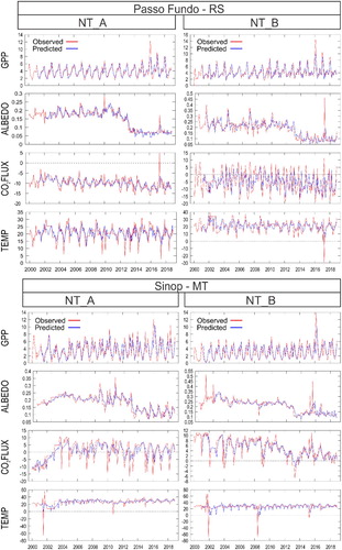
Based on the statistical analyses used for the model validation step, we verified that the model successfully simulated the time series for CO₂Flux, Albedo, GPP, and Temperature. The relationship of the highest coefficients of determination (R²) found in Passo Fundo-RS, in NT_A and NT_B for GPP (0.94 in 2008 and 0.91 in 2006) showed high correlation between observed and predicted with 90% of the variation explained and less than 10% of the values do not correlate. In Albedo (0.74 in 2006 and 0.59 in 2013) and Temperature (0.72 in 2004 and 0.58 in 2012), the two variables presented more than 70% of the variation explained, and CO₂Flux (0.56 in 2004 and 0.59 in 2012) less than 60% of the variation in observed values was explained by the predicted ones.

In Sinop – MT, the ratio of GPP (0.82 in 2017 and 0.91 in 2005) showed a high correlation, which was higher than 80% of the observed variation and less than 20% does not correlate, followed by Albedo (0.70 in 2014 and 0.64 in 2004) and CO₂Flux (0.65 in 2014 and 0.62 in 2004), which showed more than 60% of the observed variation, and Temperature (0.54 in 2011 and 0.39 in 2018), with the lowest correlation among all variables, analyzed.

Over the 19 years and of the 16 variables analyzed between the two municipalities and the two management systems, from the 304 values of R², only 193 presented R² < 0.5, which demonstrates that the variation in observed data explained 36.5% of the variation in predicted data and that 63.5% of the predicted data do not have a correlation. The d index was approximately 0.99 for all years of the time series (Figure 9). The results obtained from the regression showed a positive linear correlation for all years of the studied data series, revealing that ARIMA model is able to represent the condition of each variable in each municipality and the soil management systems in the soybean crop.

Figure 9. Observed and predicted data for Albedo, CO₂Flux (μmol m⁻² s⁻¹), GPP (g C m⁻² d⁻¹), and Temperature (°C) from January 2000 to December 2018.

Regarding the GPP in the two municipalities, it can be seen that the data are more clustered and closer to the line presenting R2 = 0.90, the highest of the series, and coefficient d = 1 (Figure 10). The variables Albedo (R² = 0.00058), CO₂Flux (R² = 0.0025), and Temperature (R² = 0.0010) had low correlation, respectively. For the entire time series studied in the two municipalities, SEE was satisfactory, with a mean value of 0.82.

Figure 10. Gross Primary Productivity (GPP) predicted versus observed among 2011 to 2018 years in NT_A and NT_B of Sinop (A and B, respectively), and NT_A and NT_B of Passo Fundo (C and D, respectively).

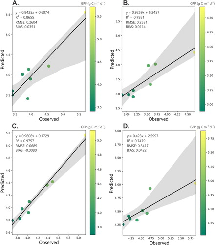
Figure 10 contains the relationship between predicted GPP versus observed GPP. The results of the presented statistical parameters (R², RMSE and BIAS) demonstrate that there is a high linear relationship between the observed and predicted values of GPP confirmed by the high values of R² and low values of RMSE and BIAS. It is important to highlight that NT_A presented a slight superiority in terms of the quality of the adjustment in relation to NT_B.

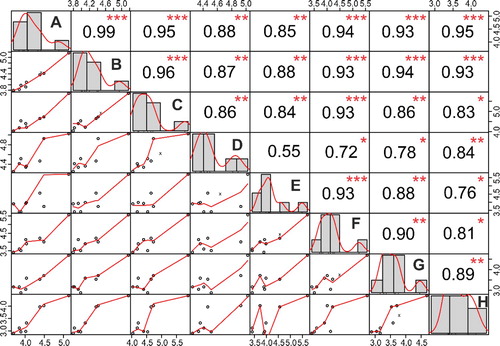
When assessing the distribution of observed and predicted data from GPP by histogram from 2011 to 2018 for validation of future data in the study area, a polygonal of variable frequencies could be generated (Figure 11). Figure 11 shows the LOESS curve demonstrating the data dispersion, in which observed NT_A of Passo Fundo – RS obtained the best dispersion followed by the best correlation. Otherwise, observed NT_A for Sinop – MT and predicted NT_B for Passo Fundo – RS had the worst dispersions and correlations between the data.

Figure 11. Histogram of each variable on the diagonal, the dispersion by the LOESS curve on the left, and the correlation of values (A – NT_A observed for Passo Fundo; B – NT_A predicted for Passo Fundo; C – NT_B observed for Passo Fundo; D – NT_B predicted for Passo Fundo; E – NT_A observed for Sinop; F – NT_A predicted for Sinop; G – NT_B observed for Sinop; H – NT_B predicted for Sinop) on the right.

Recent studies have focused predominantly on predicting the biomass energy (Wang et al. 2017), drought (Han, Wang, and Zhang 2010) or rainfall (Duffy et al. 2015; Rizeei, Pradhan, and Saharkhiz 2018), river flood analysis, and short-term predictions for future series (Machekposhti et al. 2017) and a strong performance on river flow (Fashae et al. 2019). Our study used the ARIMA (Autoregressive Integrated Moving Average) model as a prediction tool. This model can be applied to time-series data in a useful way to understand the data set better or to predict subsequent points to improve prediction accuracy in the short and medium-term.

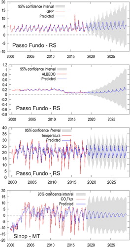
After the validation results, the variability of CO₂Flux, albedo, GPP and temperature was simulated for the future scenario from January 2019 to December 2028 based on the ARIMA model (Figure 12). The ARIMA model was able to represent the seasonality of the future period of environmental variables of both municipalities evaluated. The results of the predictions showed that the variation of GPP and albedo values for the two study sites would gradually increase until 2028. The temperature remained constant between the range of its seasonality, and CO₂Flux tends to decrease in its seasonality, indicating a higher CO₂ absorption.

Figure 12. ARIMA model applied to environmental variables: albedo, CO₂Flux, GPP, and temperature for the municipalities of Sinop – MT and Passo Fundo – RS, with a 95% confidence level.

4. Conclusion

The soybean production chain in Brazil has offered to its international consumers the image of a soybean produced with sustainability. This is a complex task, considering the territorial dimensions of the country, with soybean growing in different latitudes and cultivation methods. Our results show that a more sustainable soybean growing would be obtained by using the no-till (NT) technique, which showed adequate CO₂Flux sustainability indices in both study areas. The NT_A and NT_B values for the two study areas are always lower than tillage (T).

The environmental dynamics of the municipalities of Sinop – MT and Passo Fundo – RS is strongly linked to soybean cultivation. The CO₂Flux and GPP variables studied over 19 years are distinct between the two municipalities when considering no-till. In the municipality of Sinop, we found higher values of CO₂Flux, revealing that the Passo Fundo presents a higher absorption of CO₂ due to differences between latitudes. When we consider GPP from 2000 to 2004, the values of Passo Fundo are higher than Sinop. However, when we consider from 2005 to 2018, Sinop showed higher values, which indicates that Sinop was stimulated to soybean growing from 2005.

Future modeling based on the ARIMA model shows that seasonal trends of the environmental variables analyzed are changed due to soil management and crop implementation. The ARIMA model applied to the time series shows a confidence level for the future soybean scenario in the study areas, since there is an increasing trend in GPP, followed by a considerable decrease in albedo, CO₂Flux, and temperature in the two municipalities for the next years.

Availability statement

Data available on request from the authors.

Acknowledgments

This study was financed in part by the Coordenacao de Aperfeicoamento de Pessoal de Nivel Superior - Brasil (CAPES) - Finance Code 001 and the National Council for Research and Development (CNPq).

Disclosure statement

No potential conflict of interest was reported by the author(s).

References

- Allen, R., W. Bastiaanssen, R. Waters, M. Tasumi, and R. Trezza. 2002. “Surface Energy Balance Algorithms for Land (SEBAL)”, Idaho implementation - Advanced training and users manual, version 1.0, 97p. 2002.
- Alliaume, F., W. A. H. Rossing, P. Tittonell, G. Jorge, and S. Dogliotti. 2014. “Reduced Tillage and Cover Crops Improve Water Capture and Reduce Erosion of Fine Textured Soils in Raised bed Tomato Systems.” Agriculture, Ecosystems & Environment 183: 127–137.
- Alvarenga, R. C., W. A. L. Cabezas, J. C. Cruz, and D. P. Santana. 2001. “Ground Cover Plants for No-Till System.” Embrapa Milho e Sorgo-Artigo em periódico indexado (ALICE).
- Barnes, M. L., D. D. Breshears, D. J. Law, W. J. Van Leeuwen, R. K. Monson, A. C. Fojtik, G. A. Barron-Gafford, and D. J. Moore. 2017. “Beyond Greenness: Detecting Temporal Changes in Photosynthetic Capacity with Hyperspectral Reflectance Data.” PLoS One 12 (12): e0189539.
- Barut, Z., and I. Celik. 2017. “Tillage Effects on Some Soil Physical Properties in a Semi-Arid Mediterranean Region of Turkey.” Chemical Engineering Transactions 58: 217–222.
- Bastiaanssen, W. G. M. 2000. “SEBAL-based Sensible and Latent Heat Fluxes in the Irrigated Gediz Basin. Turkey.” Journalof Hidrology 229: 87–100.
- Blaschke, T. 2010. “Object Based Image Analysis for Remote Sensing.” ISPRS Journal of Photogrammetry and Remote Sensing 65 (1): 2–16.
- Boas Dos Santos, C. V. 2017. “Spectral Modeling for Determining CO2 Flow in Preserved Caatinga Areas and in Regeneration.” Dissertation – State University of Feira de Santana. Graduate Program in Modeling in Earth and Environmental Sciences.
- Braga, A. P. 2013. “Estimation of Gross Primary Productivity in Agricultural Areas and Primary Vegetation in the cerrado by Remote Sensing.” Dissertation - Federal University of Campina Grande, Center for Technology and Natural Resources, Campina Grande.
- Carvalho, J. L. N., J. C. Avanzi, M. L. N. Silva, C. R. D. Mello, and C. E. P. Cerri. 2010. “Carbon Sequestration Potential in Different Biomes in Brazil.” Revista Brasileira de Ciência do Solo 34 (2): 277–290.
- Carvalho, A. M., M. M. C. Bustamante, T. R. Coser, R. L. Marchão, and J. V. Malaquias. 2016. “Nitrogen Oxides and CO2 from an Oxisol Cultivated with Corn in Succession to Cover Crops.” Pesquisa Agropecuária Brasileira 9: 1213–1222.
- Carvalho, W. P., G. J. De Carvalho, D. D. O. A. Neto, and L. G. V. Teixeira. 2013. “Agronomic Performance of Cover Crops Used in Soil Protection During Fallow Period.” Pesquisa Agropecúaria Brasileira 48 (2): 157–166.
- Castillejo-González, I. L., J. M. Pena-Barragán, M. Jurado-Expósito, F. J. Mesas-Carrascosa, and F. López-Granados. 2014. “Evaluation of Pixel-and Object-Based Approaches for Mapping Wild oat (Avena Sterilis) Weed Patches in Wheat Fields using QuickBird Imagery for Site-Specific Management.” European Journal of Agronomy 59: 57–66.
- Chai, G., J. Wang, G. Wang, L. Kang, M. Wu, and Z. Wang. 2019. “Estimating Fractional Cover of non-Photosynthetic Vegetation in a Typical Grassland Area of Northern China Based on Moderate Resolution Imaging Spectroradiometer (MODIS) Image Data.” International Journal of Remote Sensing 40 (23): 8793–8810.
- CONAB - National Supply Company. 2019. “Grain Planting and Harvesting Calendar in Brazil 2019.” Accessed November 5, 2019. <https://www.ibge.gov.br/cidades-e-estados/mt.html>.
- Crowell, S. M., S. Randolph Kawa, E. V. Browell, D. M. Hammerling, B. Moore, K. Schaefer, and S. C. Doney. 2018. “On the Ability of Space-Based Passive and Active Remote Sensing Observations of CO2 to Detect Flux Perturbations to the Carbon Cycle.” Journal of Geophysical Research: Atmospheres 123 (2): 1460–1477.
- Cruz, A. P. D., and G. M. Tumibay. 2019. “Predicting Tuberculosis Treatment Relapse: A Decision Tree Analysis of J48 for Data Mining.” Journal of Computer and Communications 7 (7): 243–251.
- Czarnogorska, M., S. V. Samsonov, and D. J. White. 2016. “Airborne and Spaceborne Remote Sensing Characterization for Aquistore Carbon Capture and Storage Site.” Canadian Journal of Remote Sensing 42 (3): 274–290.
- Dai, J., D. Roberts, P. Dennison, and D. Stow. 2018. “Spectral-Radiometric Differentiation of Non-Photosynthetic Vegetation and Soil Within Landsat and Sentinel 2 Wavebands.” Remote Sensing Letters 9 (8): 733–742.
- Das, A., P. K. Ghosh, R. Lal, R. Saha, and S. Ngachan. 2017. “Soil Quality Effect of Conservation Practices in Maize–Rapeseed Cropping System in Eastern Himalaya.” Land Degradation & Development 28 (6): 1862–1874.
- De Castro, A. I., F. López-Granados, and M. Jurado-Expósito. 2013. “Broad-scale Cruciferous Weed Patch Classification in Winter Wheat using QuickBird Imagery for in-Season Site-Specific Control.” Precision Agriculture 14 (4): 392–413.
- Definiens. 2006. Definiens Professional 5: Reference Book. Munich, Germany: The Imaging Intelligence Company, p.122.
- Delgado, R. C., M. G. Pereira, P. E. Teodoro, G. L. Dos Santos, D. C. De Carvalho, I. C. Magistrali, and R. S. Vilanova. 2018. “Seasonality of Gross Primary Production in the Atlantic Forest of Brazil.” Global Ecology and Conservation 14: e00392.
- Dexter, A. R., G. Richard, D. Arrouays, E. A. Czyż, C. Jolivet, and O. Duval. 2008. “Complexed Organic Matter Controls Soil Physical Properties.” Geoderma 144 (3–4): 620–627.
- Didoné, E. J., J. P. G. Minella, J. M. Reichert, G. H. Merten, L. Dalbianco, C. A. P. De Barrros, and R. Ramon. 2014. “Impact of no-Tillage Agricultural Systems on Sediment Yield in two Large Catchments in Southern Brazil.” Journal of Soils and Sediments 14 (7): 1287–1297.
- Du, C., H. Ren, Q. Qin, J. Meng, and S. Zhao. 2015. “A Practical Split-Window Algorithm for Estimating Land Surface Temperature from Landsat 8 Data.” Remote Sensing 7 (1): 647–665.
- Duffy, P. B., P. Brando, G. P. Asner, and C. B. Field. 2015. “Projections of Future Meteorological Drought and wet Periods in the Amazon.” Proceedings of the National Academy of Sciences 112 (43): 13172–13177.
- Duval, M. E., J. M. Martinez, and J. A. Galantini. 2020. “Assessing Soil Quality Indices Based on Soil Organic Carbon Fractions in Different Long-Term Wheat Systems Under Semiarid Conditions.” Soil Use and Management 36 (1): 71–82.
- Easterling, D. R., G. A. Meehl, C. Parmesan, S. A. Changnon, T. R. Karl, and L. O. Mearns. 2000. “Climate Extremes: Observations, Modeling, and Impacts.” Science 289 (5487): 2068–2074.
- Fashae, O. A., A. O. Olusola, I. Ndubuisi, and C. G. Udomboso. 2019. “Comparing ANN and ARIMA Model in Predicting the Discharge of River Opeki from 2010 to 2020.” River Research and Applications 35 (2): 169–177.
- Field, C. B., J. T. Randerson, and C. M. Malmström. 1995. “Global net Primary Production: Combining Ecology and Remote Sensing.” Remote Sensing of Environment 51 (1): 74–88.
- Gamon, J., L. Serrano, and J. S. Surfus. 1997. “The Photochemical Reflectance Index: an Optical Indicator of Photosynthetic Radiation use Efficiency Across Species, Functional Types, and Nutrient Levels.” Oecologia 112 (4): 492–501.
- Gao, J., Z. Yu, L. Wang, and H. Vejre. 2019. “Suitability of Regional Development Based on Ecosystem Service Benefits and Losses: A Case Study of the Yangtze River Delta Urban Agglomeration, China.” Ecological Indicators 107: 105579.
- Garcia-Pedrero, A., C. Gonzalo-Martin, D. Fonseca-Luengo, and M. Lillo-Saavedra. 2015. “A GEOBIA Methodology for Fragmented Agricultural Landscapes.” Remote Sensing 7 (1): 767–787.
- Gholizadeh, A., D. Žižala, M. Saberioon, and L. Borůvka. 2018. “Soil Organic Carbon and Texture Retrieving and Mapping using Proximal, Airborne and Sentinel-2 Spectral Imaging.” Remote Sensing of Environment 218: 89–103.
- Gomes, H. B. 2009. “Radiation and Energy Balance in Sugar Cane and Cerrado Cultivation Areas in the State of São Paulo using Orbital Images.” 125p. Thesis – Federal University of Campina Grande (UFCG). Campina Grande.
- Gusso, A., J. R. Ducati, M. R. Veronez, D. Arvor, and L. G. D. Silveira Junior. 2013. “Spectral Model for Soybean Yield Estimate using MODIS/EVI Data.” International Journal of Geosciences 4 (9): 1233–1241.
- Han, P., P. X. Wang, and S. Y. Zhang. 2010. “Drought Forecasting Based on the Remote Sensing Data using ARIMA Models.” Mathematical and Computer Modelling 51 (11–12): 1398–1403.
- Haralick, R. M., K. Shanmugam, and I. H. Dinstein. 1973. “Textural Features for Image Classification.” IEEE Transactions on Systems, Man, and Cybernetics 6: 610–621.
- He, T., S. Liang, D. Wang, Y. Cao, F. Gao, Y. Yu, and M. Feng. 2018. “Evaluating Land Surface Albedo Estimation from Landsat MSS, TM, ETM+, and OLI Data Based on the Unified Direct Estimation Approach.” Remote Sensing of Environment 204: 181–196.
- Heinsch, F. A., M. Reeves, P. Votava, S. Y. Kang, C. Milesi, M. S. Zhao, J. Glassy, et al. 2003. “GPP and NPP (MOD17A2/A3) products nasa MODIS land algorithm.” MOD 17, User's Guide, p. 1–57.
- IBGE - Brazilian Institute of Geography and Statistics. 2020. “Discover Cities and States in Brazil.” Accessed January 22, 2020. <https://cidades.ibge.gov.br/>.
- Jiang, Z., A. R. Huete, K. Didan, and T. Miura. 2008. “Development of a two-Band Enhanced Vegetation Index Without a Blue Band.” Remote Sensing of Environment 112: 3833–3845.
- Jozdani, S. E., B. A. Johnson, and D. Chen. 2019. “Comparing Deep Neural Networks, Ensemble Classifiers, and Support Vector Machine Algorithms for Object-Based Urban Land use/Land Cover Classification.” Remote Sensing 11 (14): 1713.
- Kalmegh, S. 2015. “Analysis of Weka Data Mining Algorithm Reptree, Simple Cart and Randomtree for Classification of Indian News.” International Journal of Innovative Science, Engineering & Technology 2 (2): 438–446.
- Kastens, J. H., J. C. Brown, A. C. Coutinho, C. R. Bishop, and J. C. D. Esquerdo. 2017. “Soy Moratorium Impacts on Soybean and Deforestation Dynamics in Mato Grosso, Brazil.” PLoS One 12 (4): e0176168.
- Kavzoglu, T., and H. Tonbul. 2017. “A Comparative Study of Segmentation Quality for Multi-Resolution Segmentation and Watershed Transform.” In 2017 8th International Conference on Recent Advances in Space Technologies (RAST). IEEE. p. 113–117.
- Lal, R. 2015. “Restoring Soil Quality to Mitigate Soil Degradation.” Sustainability 7 (5): 5875–5895.
- Lal, R. 2016. “Soil Health and Carbon Management.” Food and Energy Security 5 (4): 212–222.
- La Scala, Jr., N., A. Lopes, J. Marques, Jr., and G. T. Pereira. 2001. “Carbon Dioxide Emissions After Application of Tillage Systems for a Dark Red Latosol in Southern Brazil.” Soil and Tillage Research 62 (3–4): 163–166.
- Liu, T., A. Abd-Elrahman, J. Morton, and V. L. Wilhelm. 2018. “Comparing Fully Convolutional Networks, Random Forest, Support Vector Machine, and Patch-Based Deep Convolutional Neural Networks for Object-Based Wetland Mapping using Images from Small Unmanned Aircraft System.” GIScience & Remote Sensing 55 (2): 243–264.
- LÓPEZ-GRANADOS, F. 2011. “Weed Detection for Site-Specific Weed Management: Mapping and Real-Time Approaches.” Weed Research 51 (1): 1–11.
- Machekposhti, K. H., H. Sedghi, A. Telvari, and H. Babazadeh. 2017. “Flood Analysis in Karkheh River Basin using Stochastic Model.” Civil Engineering Journal 3 (9): 794–808.
- Marsett, R. C., J. Qi, P. Heilman, S. H. Biedenbender, M. C. Watson, S. Amer, M. Weltz, D. Goodrich, and R. Marsett. 2006. “Remote Sensing for Grassland Management in the Arid Southwest.” Rangeland Ecology & Management 59 (5): 530–540.
- Martins, L. N., and G. M. M. Baptista. 2013. “Multitemporal Analysis of Forest Carbon Sequestration in the Carão Settlement Project, Acre.” Revista Brasileira de Geografia Física 6 (6): 1648–1657.
- Moraes Novo, E. M. L. de. 2010. Remote Sensing: Principles and Applications. 4ª Ed. São Paulo: Blucher, 363p.
- Nanni, M. R., and J. A. M. Demattê. 2006. “Behavior of the Soil Line Obtained by Laboratory Spectroradiometry for Different Soil Classes.” Revista Brasileira de Ciência do Solo 30 (6): 1031–1038.
- Novo, E. M. L. D. M., L. G. Ferreira, C. Barbosa, C. Carvalho, E. E. Sano, Y. Shimabukuro, J. J. Melack, et al. 2005. “Advanced Remote Sensing Techniques Applied to the Study of Climate Change and the Functioning of Amazonian Ecosystems.” Acta Amazonica 35 (2): 259–272.
- Ouyang, W., X. Wan, Y. Xu, X. Wang, and C. Lin. 2020. “Vertical Difference of Climate Change Impacts on Vegetation at Temporal-Spatial Scales in the Upper Stream of the Mekong River Basin.” Science of The Total Environment 701: 134782.
- Pastick, N. J., D. Dahal, B. K. Wylie, S. Parajuli, S. P. Boyte, and Z. Wu. 2020. “Characterizing Land Surface Phenology and Exotic Annual Grasses in Dryland Ecosystems Using Landsat and Sentinel-2 Data in Harmony.” Remote Sensing 12 (4): 725.
- Ponzoni, F. J., Y. E. Shimabukuro, and T. M. Kuplich. 2012. Remote Sensing of Vegetation. 2nd ed. São Paulo: Oficina de Textos, 176p.
- Qi, J., R. Marsett, P. Heilman, S. Bieden-Bender, S. Moran, D. Goodrich, and M. Weltz. 2002. “Ranges Improves Satellite-Based Information and Land Cover Assessments in Southwest United States.” EOS, Transactions American Geophysical Union 83 (51): 601–606.
- Rahman, A. F., J. A. Gamon, D. A. Fuentes, D. A. Roberts, and D. Prentiss. 2001. “Modeling Spatially Distributed Ecosystem Flux of Boreal Forest using Hyperspectral Indices from AVIRIS Imagery.” Journal of Geophysical Research 106 (D24): 33579–33591.
- Ramírez, P. B., F. J. Calderón, S. J. Fonte, F. Santibáñez, and C. A. Bonilla. 2020. “Spectral Responses to Labile Organic Carbon Fractions as Useful Soil Quality Indicators Across a Climatic Gradient.” Ecological Indicators 111: 106042.
- R Core Team. 2015. “R: A Language and Environment for Statistical Computing.” 583. Vienna, Austria: R Foundation for Statistical Computing.
- Reicosky, D. C., T. J. Sauer, and J. L. Hatfield. 2011. “Challenging Balance between Productivity and Environmental Quality: Tillage Impacts.” Publications from USDA-ARS / UNL Faculty, 1373. https://digitalcommons.unl.edu/usdaarsfacpub/1373.
- Ren, H., C. Du, R. Liu, Q. Qin, G. Yan, Z. L. Li, and J. Meng. 2015. “Atmospheric Water Vapor Retrieval from Landsat 8 Thermal Infrared Images.” Journal of Geophysical Research: Atmospheres 120 (5): 1723–1738.
- Richey, J. E., J. M. Melack, A. K. Aufdenkampe, V. M. Ballester, and L. L. Hess. 2002. “Outgassing from Amazonian Rivers and Wetlands as a Large Tropical Source of Atmospheric CO2.” Nature 416 (6881): 617–620.
- Rizeei, H. M., B. Pradhan, and M. A. Saharkhiz. 2018. “Surface Runoff Prediction Regarding LULC and Climate Dynamics using Coupled LTM, Optimized ARIMA, and GIS-Based SCS-CN Models in Tropical Region.” Arabian Journal of Geosciences 11 (3): 53.
- Rossi, F. S., C. A. Silva Junior, J. F. Oliveira-Júnior, P. E. Teodoro, L. S. Shiratsuchi, M. Lima, L. P. R. Teodoro, A. V. Tiago, and G. F. Capristo-Silva. 2020. “Identification of Tillage for Soybean Crop by Spectro-Temporal Variables, GEOBIA, and Decision Tree.” Remote Sensing Applications: Society and Environment 19: 100356.
- Rouse, J. W., R. H. Hass, J. A. Schell, and D. W. Deering. 1974. “Monitoring Vegetation Systems in the Great Plains with ERTS.” In EARTH RESOURCES TECHNOLOGY SATELLITE SYMPOSIUM, 3., Washington. Proceedings. Washington: NASA, 1974. p. 309–317.
- Shang, M., S. Wang, Y. Zhou, C. Du, and W. Liu. 2019. “Object-Based Image Analysis of Suburban Landscapes using Landsat-8 Imagery.” International Journal of Digital Earth 12 (6): 720–736.
- Silva, B. B., A. C. Braga, C. C. Braga, L. M. M. Oliveira, S. M. G. L. Montenegro, and B. Barbosa Junior. 2016. “Procedures for Calculation of the Albedo with OLI-Landsat 8 Images: Application to the Brazilian Semi-Arid.” Revista Brasileira de Engenharia Agrícola e Ambiental 20 (1), 3–8. doi:10.1590/1807-1929/agriambi.v20n1p3-8.
- Silva, L. C., and H. Lambers. 2020. “Soil-plant-atmosphere Interactions: Structure, Function, and Predictive Scaling for Climate Change Mitigation.” Plant and Soil 461: 5–27
- Silva, B. B., G. M. Lopes, and P. V. Azevedo. 2005. “Radiation Balance in Irrigated Areas using Landsat 5-TM Images.” Revista Brasileira de Meteorologia 20 (2): 243–252.
- Silva Junior, C. A., G. M. Costa, F. S. Rossi, J. C. E. Vale, R. B. Lima, M. G. Lima, J. F. Oliveira-Junior, P. E. Teodoro, and R. C. Santos. 2019a. “Remote Sensing for Updating the Boundaries Between the Brazilian Cerrado-Amazonia Biomes.” Environmental Science & Policy 101: 383–392.
- Silva Junior, C. A., A. H. S. Leonel Junior, F. S. Rossi, W. L. F. Correia Filho, D. B. Santiago, J. F. Oliveira-Junior, P. E. Teodoro, M. G. Lima, and G. F. Capristo-Silva. 2020. “Mapping Soybean Planting Area in Midwest Brazil with Remotely Sensed Images and Phenology-Based Algorithm using the Google Earth Engine Platform.” Computers And Electronics in Agriculture 169: 105194.
- Silva Junior, C. A., and M. Lima. 2018. “Soy Moratorium in Mato Grosso: Deforestation Undermines the Agreement.” Land Use Policy 71: 540–542.
- Silva Junior, C. A. D., M. R. Nanni, J. F. D. Oliveira-Júnior, E. Cezar, P. E. Teodoro, R. C. Delgado, S. Shiratsuchi L, M. Shakir, and M. L. Chicati. 2019b. “Object-based Image Analysis Supported by Data Mining to Discriminate Large Areas of Soybean.” International Journal of Digital Earth 12 (3): 270–292.
- Silva Junior, C. A., M. R. Nanni, P. E. Teodoro, and G. F. C. Silva. 2017. “Vegetation Indices for Discrimination of Soybean Areas: A new Approach.” Agronomy Journal 109 (4): 1331–1343.
- Silva-Olaya, A. M., C. E. P. Cerri, N. La Scala, Jr., C. T. D. S. Dias, and C. C. Cerri. 2013. “Carbon Dioxide Emissions Under Different Soil Tillage Systems in Mechanically Harvested Sugarcane.” Environmental Research Letters 8 (1): 015014.
- SOJAMAPS. 2020. “Geotechnology Applied in Agriculture and Forest (GAAF).” Accessed January 05, 2020. <http://pesquisa.unemat.br/gaaf/sojamaps/>.
- Solman, S. A., M. N. Nunez, and M. F. Cabré. 2008. “Regional Climate Change Experiments Over Southern South America. I: Present Climate.” Climate Dynamics 30 (5): 533–552.
- Souza, A. P., L. L. Mota, T. Zamadei, C. C. Martim, F. T. Almeida, and J. Paulino. 2013. “Climatic Classification and Climatological Water Balance in the State of Mato Grosso.” Nativa 1 (1): 34–43.
- Souza-Filho, P., W. Nascimento, D. Santos, E. Weber, R. Silva, and J. Siqueira. 2018. “A GEOBIA Approach for Multitemporal Land-Cover and Land-use Change Analysis in a Tropical Watershed in the Southeastern Amazon.” Remote Sensing 10 (11): 1683.
- Spera, S. A., G. L. Galford, M. T. Coe, M. N. Macedo, and J. F. Mustard. 2016. “Land-use Change Affects Water Recycling in Brazil's Last Agricultural Frontier.” Global Change Biology 22 (10): 3405–3413.
- Tasumi, M., R. G. Allen, R. Trezza, and J. L. Wright. 2008. “Satellite-Based Energy Balance to Assess Within-Population Variance of Crop Coefficient Curves.” Journal of Irrigation and Drainage Engineering 131: 94–108.
- Tavares, R. L. M., S. R. D. M. Oliveira, F. M. M. D. Barros, C. V. V. Farhate, Z. M. D. Souza, S. Junior, and N. La. 2018. “Prediction of Soil CO2 Flux in Sugarcane Management Systems using the Random Forest Approach.” Scientia Agricola 75 (4): 281–287.
- USGS (United Stated Geological Survey). 2019. “Using the USGS Landsat 8 Product.” Accessed October 04, 2019. <https://landsat.usgs.gov/using-usgs-landsat-8-product>.
- Valipour, M. 2015. “Long-Term Runoff Study using SARIMA and ARIMA Models in the United States.” Meteorological Applications 22 (3): 592–598.
- Van Deventer, A. P., A. D. Ward, P. H. Gowda, and J. G. Lyon. 1997. “Using Thematic Mapper Data to Identify Contrasting Soil Plains and Tillage Practices.” Photogrammetric Engineering and Remote Sensing 63: 87–93.
- Vogels, M. F., S. M. De Jong, G. Sterk, H. Douma, and E. A. Addink. 2019. “Spatio-temporal Patterns of Smallholder Irrigated Agriculture in the Horn of Africa using GEOBIA and Sentinel-2 Imagery.” Remote Sensing 11 (2): 143.
- Wang, Z., A. M. Erb, C. B. Schaaf, Q. Sun, Y. Liu, Y. Yang, and M. O. Román. 2016. “Early Spring Post-Fire Snow Albedo Dynamics in High Latitude Boreal Forests using Landsat-8 OLI Data.” Remote Sensing of Environment 185: 71–83.
- Wang, X., X. Gao, X. Zhang, W. Wang, and F. Yang. 2020. “An Automated Method for Surface Ice/Snow Mapping Based on Objects and Pixels from Landsat Imagery in a Mountainous Region.” Remote Sensing 12 (3): 485.
- Wang, W., W. Ouyang, F. Hao, and G. Liu. 2017. “Temporal-Spatial Variation Analysis of Agricultural Biomass and its Policy Implication as an Alternative Energy in Northeastern China.” Energy Policy 109: 337–349.
- Wang, G., J. Wang, X. Zou, G. Chai, M. Wu, and Z. Wang. 2019. “Estimating the Fractional Cover of Photosynthetic Vegetation, non-Photosynthetic Vegetation and Bare Soil from MODIS Data: Assessing the Applicability of the NDVI-DFI Model in the Typical Xilingol Grasslands.” International Journal of Applied Earth Observation and Geoinformation 76: 154–166.
- Wick, B., R. F. Kühne, and P. L. Vlek. 1998. “Soil Microbiological Parameters as Indicators of Soil Quality Under Improved Fallow Management Systems in South-Western Nigeria.” Plant and Soil 202 (1): 97–107.
- Wu, L., Q. Qin, X. Liu, H. Ren, J. Wang, X. Zheng, X. Ye, and Y. Sun. 2016. “Spatial up-Scaling Correction for Leaf Area Index Based on the Fractal Theory.” Remote Sensing 8 (3): 197.
- Xi, W., S. Du, Y. C. Wang, and X. Zhang. 2019. “A Spatiotemporal Cube Model for Analyzing Satellite Image Time Series: Application to Land-Cover Mapping and Change Detection.” Remote Sensing of Environment 231: 111212.
- Yang, L., L. R. Mansaray, J. Huang, and L. Wang. 2019. “Optimal Segmentation Scale Parameter, Feature Subset and Classification Algorithm for Geographic Object-Based Crop Recognition using Multisource Satellite Imagery.” Remote Sensing 11 (5): 514.
- Yin, H., A. Khamzina, D. Pflugmacher, and C. Martius. 2017. “Forest Cover Mapping in Post-Soviet Central Asia using Multi-Resolution Remote Sensing Imagery.” Scientific Reports 7 (1): 1–11.
- Yue, J., Q. Tian, X. Dong, K. Xu, and C. Zhou. 2019. “Using Hyperspectral Crop Residue Angle Index to Estimate Maize and Winter-Wheat Residue Cover: A Laboratory Study.” Remote Sensing 11 (7): 807.