Nyström-based spectral clustering using airborne LiDAR point cloud data for individual tree segmentation

ABSTRACT

The spectral clustering method has notable advantages in segmentation. But the high computational complexity and time consuming limit its application in large-scale and dense airborne Light Detection and Ranging (LiDAR) point cloud data. We proposed the Nyström-based spectral clustering (NSC) algorithm to decrease the computational burden. This novel NSC method showed accurate and rapid in individual tree segmentation using point cloud data. The K-nearest neighbour-based sampling (KNNS) was proposed for the Nyström approximation of voxels to improve the efficiency. The NSC algorithm showed good performance for 32 plots in China and Europe. The overall matching rate and extraction rate of proposed algorithm reached 69% and 103%. For all trees located by Global Navigation Satellite System (GNSS) calibrated tape-measures, the tree height regression of the matching results showed an value of 0.88 and a relative root mean square error (RMSE) of 5.97%. For all trees located by GNSS calibrated total-station measures, the values were 0.89 and 4.49%. The method also showed good performance in a benchmark dataset with an improvement of 7% for the average matching rate. The results demonstrate that the proposed NSC algorithm provides an accurate individual tree segmentation and parameter estimation using airborne LiDAR point cloud data.

KEYWORDS:

• Tree segmentation
• airborne LiDAR
• spectral clustering
• Nyström approximation
• sampling method

1. Introduction

The research of tree segmentation helps gaining a comprehensive understanding of the complex structure as well as various biophysical processes of forests. Light Detection and Ranging (LiDAR), an active remote sensing technology, can obtain not only high-precision forest spatial structure information but also information under canopy topographic by transmitting laser energy and receiving return signals. This technology has unparalleled advantages of passive remote sensing and is therefore widely applied into forest management and ecosystem research (Hyyppä et al. 2000). Individual tree segmentation algorithms using LiDAR data can be mainly divided into two categories. One is surface model methods that utilize the canopy height model (CHM). The other is three-dimensional (3D) methods which utilize information of the whole point cloud (Zhao et al. 2014; Lindberg and Holmgren 2017). The 3D methods can be further categorized into point-based methods which directly utilize the original or normalized point cloud, and voxel-based methods which project the point cloud into the voxel space in order to increase computational efficiency.

The basic idea of surface model methods is to segment individual trees by deriving a surface model that represents the upper contour of the canopy and identifying the local maxima in the surface as treetops (Lindberg and Holmgren 2017). When searching the local maxima in CHM, fixed or variable window sizes that depend on factors such as crown width and stand density (Zimble et al. 2003) are used. Popescu, Wynne, and Nelson (2002) determined the different sizes of window by calculating the crown width from the linear regression of tree height. Zimble et al. (2003) utilized a circular search window with a fixed radius according to the measured minimum crown width. Chen et al. (2006) applied marker-controlled watershed segmentation to isolate individual trees using the treetops detected in CHM by variable window sizes. Zhao et al. (2014) used a morphological crown control-based watershed algorithm to isolate individual trees in the closed coniferous forest. Some other surface model methods were based on the existing 2D image segmentation methods (Brandtberg et al. 2003).

Clustering methods have been widely used for individual tree segmentation based on point methods. Morsdorf et al. (2004) extracted the local maxima from the digital surface model (DSM) as seed points for $k$-means clustering analysis to segment individual trees. Gupta, Weinacker, and Koch (2010) compared several improved k-means clustering and hierarchical clustering on crown extraction. It was found that using local maxima as seed points and scaling down the height value could improve results. Furthermore, the results of the hierarchical clustering method were not satisfactory compared to various $k$-means methods. In addition to clustering methods, there are many other 3D methods developed for individual tree segmentation. Lee et al. (2010) utilized the region growing method from the treetops downward to the whole point cloud. Sačkov et al. (2017) proposed a method that included several restriction rules on the tree height and crown width to increase the probability of detecting the actual tree. Williams et al. (2020) developed a multiclass graph cut algorithm alongside knowledge of crown allometries to complete the individual tree crown detection.

Regarding voxel-based methods, cubes with a given resolution were usually used to construct the voxel cloud. Wang et al. (2016) employed a voxel resolution of 0.5 m × 0.5 m × 0.5 m. They defined the centre of each voxel element within the voxel as the position and the number of points as the weight of that voxel. Ayrey et al. (2017) proposed a layer stacking method, which included the main steps of horizontal layering, k-means clustering, and layer stacking. Shi and Malik (2000) proposed the normalized cut (NCut) method, which divided data into groups based on the spatial similarity between points. On this basis, Reitberger et al. (2009) implemented a new 3D segmentation of individual trees using NCut segmentation. The features were the distance between two voxels as well as the mean intensity and the mean pulse width for each voxel. Yao, Krzystek, and Heurich (2012) used the segmentation results of the NCut method to classify tree species and complete the estimation of stem volume and DBH.

For the surface model methods, the utilization of upper canopy surface with a small data volume makes it efficient even for large scale individual tree segmentation. However, accurate results were projected only for simple, uniform forest types with the loss of understory information. Moreover, the results rely heavily on the priori information, such as the width for the window size to identify local maxima in CHM. 3D methods using the whole point cloud information are expected to produce more accurate individual tree segmentation results, especially for those stands with complex vertical structure. Nevertheless, there are still some challenges: (i) the reliance on the priori information, e.g. the assumed tree position for the initial seed point for $k$-means clustering; (ii) the restrictions on the data distribution, e.g. more stable performance with Gaussian distributed variables for $k$-means clustering; (iii) the limitation of algorithm popularity because of computational complexity for large-scale data, e.g. regional growth and NCut methods. Although voxel-based methods have a good performance for the preprocessing of point cloud data, it contributes less to the reduction of the data volume.

Based on the spectral graph theory, spectral clustering methods have recently shown attractive advantages in segmentation problems (Luxburg 2007). Unlike the classic $k$-means clustering approach, there are no restrictions on data distribution for spectral clustering methods (Fowlkes et al. 2004). For the iterative two-class cut method (Reitberger et al. 2009), spectral clustering has a similar theoretical foundation but offers better effectiveness in multiclass problems (Luxburg 2007). Heinzel and Huber (2018) introduced spectral clustering in tree segmentation using dense terrestrial laser scanning data with a good performance. The biggest challenge of the spectral clustering method for LiDAR point cloud data is computational complexity. For a data set with $N$ points, $O(N^2)$ memory is needed to construct the similarity matrix, and the complexity of its eigenvectors calculation is $O(N^3)$ (Lin and Cohen 2010; Ye et al. 2016). Besides time consuming, the procedure poses the risk of memory overflow when $N$ is large for the large-scale dense LiDAR point cloud data.

Nyström approximation is an effective technique for the spectral clustering method in the application of large-scale data. It was originally designed to find a numerical solution of the eigenfunction problem (Sloan 1981). Using a sampling technique and the numerical approximation theory, the eigenvector calculated for sampled points are extended to unsampled points by interpolation weights (Fowlkes et al. 2004). Since different samples produce different approximations of the original similarity matrix, the choice of sampling method is crucial for the method performance (Bouneffouf and Birol 2015). Only when the sampled points can extract the inherent feature of the dataset, i.e. the samples are all landmark points, more ideal results can be obtained with less approximation error. Various sampling methods have been therefore proposed. Some are as simple as random sampling (RS) (Fowlkes et al. 2004; Cohen et al. 2015), which allows every point to have the same probability of being selected as a sample. Other alternative versions include $k$-means-based sampling (KS) (Zhang, Tsang, and Kwok 2008), incremental sampling (IS) (Zhang and You 2011), minimum similarity sampling (SS) (Zeng et al. 2014), etc. Bouneffouf and Birol (2015) pointed out that minimizing the sum of the squared similarities between the new and the precedent sampling points would maximize the determinant of the sampling similarity matrix, and then minimize the approximation error. Considering the variability and similarity of sampling points, the minimum sum of squared similarities (MSSS) showed a good performance in previous study (Bouneffouf and Birol 2015).

In spite of Nyström method can be used to solve the computational burden of eigenvectors, however, the dilemma in big data storage still needs to be solved. In comparison to the traditional voxel-based approach, the super voxel based method provides a more efficient approach to process point cloud data. Li and Sun (2018) used adaptive octree to acquire supporting points, and took the over segmentation results of the region growing as super voxels. Combined with the resampling process, the unorganized LiDAR point cloud was automatically refined.

In this paper, the Nyström-based spectral clustering (NSC) algorithm combined with a mean shift voxelization was applied to the individual tree segmentation for dense LiDAR point cloud data. Additionally, a more efficient sampling method based on the $k$-nearest neighbour relationship was proposed for the Nyström approximation. The assessment of the segmentation results was conducted in terms of the detection rate and the parameters of tree height. The remainder of this paper is structured as follows. Section 2 introduces the study area, airborne LiDAR data, and reference data. Section 3 describes the details of the proposed segmentation method, key control parameters, and accuracy assessment. Section 4 evaluates the results of individual tree segmentation and tree height accuracy. This section also shows the comparison of small- and large-scale segmentation as well as the analysis of parameter sensitivity. Section 5 discusses the effectiveness of the similarity function and sampling method as well as the effects of different matching methods for the accuracy assessment. Section 6 summarizes all the important findings of this study.

2. Study area and LiDAR data

2.1. Study area and field measurements

As shown in Figure 1, the three study sites are located in Mengjiagang (130°32′–130°52′ E, 46°20′–46°30′ N), Dagujia (124°44′–125°16′ E, 42°14′–42°27′ N), and Saihanba (117°–117°36′ E, 42°18′–42°36′ N) from north to south. Their terrain is a gentle slope or hilly state. Dominant tree species are the typical larch plantations, including Larix olgensis in Mengjiagang, Larix Kaempferi in Dagujia, and larix principis-rupprechtii in Saihanba. In this study, 18 plots including 1 large plot and 17 standard plots were used to verify the proposed algorithm. In addition, we selected a tile of 1 $\mathrm{k}{\mathrm{m}}^2$ (Figure 1) in Mengjiagang Forest Farm for the assessment of large area. The tile segmentation results were compared with three plots inside this area.

Figure 1. The location of study sites, the distribution of field plots and testing tile. The green circles are the plots in each Forest Farm. Upper right panel is CHM of the testing tile. Lower right panel and lower left panel are the CHM and the LiDAR point cloud of the large plot in Saihanba Forest Farm, respectively.

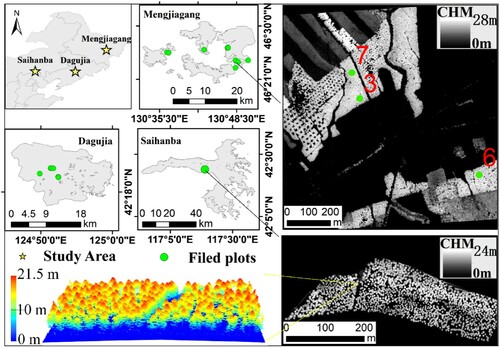
In total, 2782 living trees with a diameter at breast height (DBH) $\ge$5 cm were recorded as references. The tree height varied from 4.2 to 28.8 m. Table 1 summarizes the parameters of the field plots. DBH was measured using a PI-tape with circular object assumption. Crown sizes were measured using a tape on the ground in four directions (i.e. east, west, south, and north), and the mean value was calculated as the crown radius. The centre location of each plot was measured using a differential Global Navigation Satellite System (GNSS). For the plots from #1 to #11 in Mengjiagang Forest Farm, the stem positions were obtained by the tape and calibreated to the LiDAR CHM through post-processing method. The positioning accuracy of each single stem in plots #1–#11 was within 1 m (Liang, Pang, and Chen 2020). For the large plot #12 in Saihanba Forest Farm, the stem positions were obtained by Real Time Kinematic (RTK) GNSS system, and the tree heights were estimated using the allometric equation. For the plots #13–#18 in Dagujia Forest Farm, a number of trees were selected and their positions were measured with total station and GNSS, which have obtained the positioning accuracy within 0.5 m. Meanwhile, the tree heights in Mengjiagang and Dagujia Forest Farm were measured using ultrasonic altimeter and laser hypsometer, respectively. Besides, stem densities were categorized into three levels, i.e. high (H), medium (M) and low (L). These stem densities were resulted from selective logging activities during different growth stages of larch plantation management.

Table 1. Characteristics of 18 field plots in three study sites of China.

Plot #	Point density (pts/${\mathrm{m}}^2$)	Number of trees	Plot size (ha)	Average DBH (cm)	Average height (m)	Average crown radius (m)	Stem density (trees/ha)	Stem density class
1	14	114	0.06	11.93	13.55	1.23	1900	H
2	14	113	0.09	17.53	20.28	1.45	1256	M
3	14	73	0.06	18.15	22.24	1.26	1217	M
4	14	113	0.09	17.23	19.25	1.44	1256	M
5	10	67	0.06	17.14	17.41	1.50	1117	M
6	14	71	0.06	17.97	20.62	1.40	1183	M
7	12	65	0.06	18.86	21.31	1.42	1083	M
8	14	109	0.09	16.71	19.36	1.56	1211	M
9	14	111	0.15	21.66	22.19	1.89	740	L
10	14	82	0.15	23.85	22.82	2.45	547	L
11	14	73	0.15	25.76	24.23	2.53	487	L
12	16	1435	5.20	27.40	18.92	3.05	276	L
13^a	31	36	0.09	13.94	13.27	1.39	1111	–
14^a	34	99	0.09	15.02	19.50	1.15	1444	–
15^a	35	91	0.09	15.48	18.51	1.39	1222	–
16^a	35	18	0.09	16.61	19.57	2.00	922	–
17^a	25	76	0.09	16.49	19.49	1.93	833	–
18^a	35	36	0.09	16.23	19.02	1.97	722	–

2.2. Airborne LiDAR data

The CAF-LiCHy airborne observation system was used for the data collection (Pang et al. 2016). The Riegl LMS-Q680i scanner was integrated in the CAF-LiCHy system. The wavelength of this system was 1550 nm, with a 3 ns pulse length and 0.5 mrad beam divergence. The max pulse repetition rate of the sensor is 400 kHz. The LiDAR data parameters in the three study areas are shown in Table 2, which including the point density, flight time, relative flight height, and average flight speed (Table 2). The point density varied from 10 to 35 pts/m² after taking the overlapped flights into account.

Table 2. LiDAR data parameters of three study sites of China.

Study site	Point density (pts/${\mathrm{m}}^2$)	Above ground flight height (m)	Flight speed (km/h)	Acquisition date
Mengjiagang	10–14	900	160	31 May–15 June 2017
Dagujia	20–35	1000	180	20–28 July 2018
Saihanba	10–35	800/1000	150/130	1–19 September 2018

2.3. Benchmark dataset in the Alpine Space of Europe

In order to further examine the segmentation capability for different forest types and compare the proposed method with other approaches, we used 14 plots from the NEWFOR website (Eysn et al. 2015). These 14 plots are located in 6 different study areas in the Alpine region. The study data are heterogeneous and collected under different conditions for different purpose. The forest types in the study areas are diverse with the coniferous proportion ranging from 28% to 100%. The main tree species include spruce, fir, beech, larch, etc. The statistical description of the forest plots is shown in Table 3, where the Plot ID is consistent with the definition by Eysn et al. (2015). More detailed parameters can be found in their work.

Table 3. Statistical description of the 14 available forest plots from the NEWFOR Alpine Space Programme.

Plot #	Study area	Point density (pts/${\mathrm{m}}^2$)	Plot size (ha)	Stem density (trees/ha)	Mean height (m)	Coniferous proportion (%)	Main species	Forest class
1	Saint-Agnan, France	13	1.00	359	17.1	56	Fir, beech	ML/M
2	Cotolivier, Italy	11	0.13	843	18.1	97	Scots pine, larch, spruce	ML/C
3	Cotolivier, Italy	11	0.13	390	16.5	92	Scots pine, larch	SL/C
4	Cotolivier, Italy	11	0.13	175	12.9	59	Larch, sycamore	ML/M
6	Montafon, Austria	22	0.30	400	13.9	100	Spruce	ML/C
7	Pellizzano, Italy	95–121	0.13	374	25.6	100	Spruce, larch, fir	SL/C
8	Pellizzano, Italy	95–121	0.13	1870	13.7	80	Larch, spruce, fir, sycamore, poplar	ML/M
9	Asiago, Italy	11	0.13	708	23.6	100	Spruce, fir	SL/C
10	Asiago, Italy	11	0.13	851	16.9	80	Spruce, fir, beech	ML/M
11	Asiago, Italy	11	0.13	1344	13.9	28	Spruce, fir, beech	ML/M
15	Leskova, Slovenia	30	0.20	265	22.9	76	Fir, spruce, beech	SL/M
16	Leskova, Slovenia	30	0.20	185	24.6	78	Fir, spruce, beech	SL/M
17	Leskova, Slovenia	30	0.20	585	20.6	47	Fir, spruce, beech, sycamore, elm	ML/M
18	Leskova, Slovenia	30	0.20	460	24.6	53	Fir, beech, sycamore	ML/M

3. Methods

3.1. Segmentation method

3.1.1. Overall of the workflow

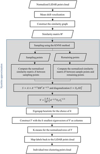
Our algorithm was based on the spectral clustering method, and its computational dilemma was solved by the mean shift voxelization and Nyström approximation. The mean shift method transformed the LiDAR point cloud into the voxel space and consequently reduced the burden of calculations and storage. The Nyström method that used the sampling technique provided a fast approximation of the eigenvalues and eigenvectors of the similarity matrix. A new sampling procedure, K-nearest neighbour-based sampling (KNNS), was proposed for the Nyström method, which further improved the performance of the sampling process. Figure 2 shows the general workflow of the algorithm, which was implemented using Python programming language. The shaded rectangle in Figure 2 is the procedure of Nyström approximation. The overall framework consists of the following main steps of (i) LiDAR point cloud pre-processing, including mean shift voxelization; (ii) constructing a similarity graph; (iii) calculating the eigenvalues and eigenvectors of the similar matrix; (iv) clustering the rows of the eigenvector matrix; and (v) mapping the results back to LiDAR point clouds and generating individual tree clusters.

Figure 2. Flowchart of individual tree segmentation using Nyström-based spectral clustering method.

3.1.2. Mean shift voxelization

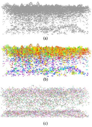
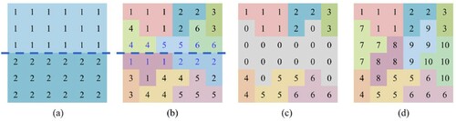
The traditional voxel-based approach transforms the point cloud into cube voxels with a given resolution. Its main advantage is the convenient access to the neighbourhood of each voxel point. However, a small resolution is usually chosen to obtain a forest structure that is highly close to the original LiDAR point cloud, which limited compression of the data volume. The super voxel based method provides alternatively a more flexible and efficient approach to constructing a tighter voxel space. Mean shift is a clustering algorithm that groups points by iteratively shifting each point towards the density maxima within a kernel. It is a robust method with fast and good results that does not need to assume the distribution of data points or the number of clusters. On account of the advantages of mean shift method, we used it to complete the voxelization procedure. As shown in Figure 3, each voxel was represented by a cluster obtained based on the mean shift. The voxel position was determined by the centre point and the voxel weight is equal to the number of points within it. As a result, mean shift voxelization reduced the amount of data by approximately a factor of 10 (Figure 3).

Figure 3. Examples of (a) the original LiDAR point cloud of plot 11 (29,671 pts), (b) the clustering result of mean shift method (each colour represents one voxel) and (c) the voxel cloud (each voxel is represented by voxel weight, 2802 pts).

3.1.3. Constructing the similarity graph

The spectral clustering algorithm offers great flexibility in the definition of a similarity function and the similarity graph. Referring to the work of Luxburg (2007), we selected the suggested $K$-nearest neighbour (KNN) graph, that is simple to construct a sparse adjacency matrix and is less susceptible to inappropriate parameter choices. Considering the shape of the trees and the properties of the voxels, we used the Gaussian similarity function as follows: (1) $s(x_i,x_j)=\{\begin{array}{cc}{e}^{-n_i{n}_j{\left({\displaystyle \frac{D_{ij}^{XY}}{{\sigma }_{xy}}}\right)}^2}\times e^{-n_i{n}_j{\left({\displaystyle \frac{D_{ij}^Z}{{\sigma }_z}}\right)}^2}& \mathrm{if}(x_j\mathrm{in}\mathrm{KNN}\mathrm{of}{x}_i)\\ 0& \mathrm{otherwise}\end{array}$(1) In this equation, $D_{ij}^{XY}$ and $D_{ij}^Z$ are the horizontal and vertical Euclidian distances between two voxels $x_i$ and $x_j$, respectively. They were assigned different scale factors ${\sigma }_{xy}$ and ${\sigma }_z$ to satisfy the ellipsoid shape of the tree. The two weighting factors $n_i$ and $n_j$ are the weights of the voxel $x_i$ and $x_j$, that are used to maintain the consistency of the voxel space with the original point cloud.

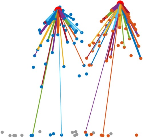
Figure 4 shows the similarity graphs of two trees. All the circle dots in the figure represent the voxels of the two trees. The big red dots are the base voxels, which are used to construct the similarity graphs. Each base voxel is connected with its $K$-nearest neighbours by line segment, and the thickness of line segment represents the similarity between the base voxel and the connected voxel. The blue and orange small circle dots represent the $K$-nearest neighbours of the two base voxels, while the grey small circle dots represent the points that are not their $K$-nearest neighbours. Different colours are used to render the connection lines for an enhanced display effect. Meanwhile, each similarity graph only connects the base voxel with odd connection points to display neatly. The even connection points have similar similarities with their neighbourhood points.

Figure 4. The similarity graph of different trees. Here, the number of $\mathrm{KNN}$ is 50. The big red circle dots represent the base voxels of different similarity graphs. The blue and orange small circle dots represent the $K$-nearest neighbours of each base voxel. The grey small circle dots represent the voxels that are not the $K$-nearest neighbours of each base voxel. Connecting lines with different thicknesses and colour represent the Gaussian similarity between the base voxel and the connected points.

To improve the searching speed of the K-nearest neighbours for the similarity matrix construction of each voxel, we employed the $kd$-tree data structure to compensate because of the lack of the location index of the voxels under mean shift voxelization. It should be noted that the similarity matrix is not symmetric, since we constructed the unilateral connected $K$-nearest neighbour graph instead of a symmetrical graph.

3.1.4. Nyström approximation

The eigenvectors and eigenvalues of the similarity matrix were computed using the Nyström method approximatively. The workflow of the Nyström method is shown in Figure 2. Its principle is illustrated in the following sections.

3.1.4.1. Nyström method

For a data set with $N$ points and a similarity matrix $W$, the Nyström method divides all the points into the n sampling points and the $m$ remaining points ($m=N-n$). Then, the similarity matrix $W$ is partitioned as: (2) $W=\left[\begin{array}{cc}A& B\\ B^T& C\end{array}\right]$(2) where $A\in {\mathbb{R}}^{n\times n}$ represents the subblock of weights among the sampling points with diagonalization $A=U\mathrm{\Lambda }{U}^T$, $B\in {\mathbb{R}}^{n\times m}$ represents the weights from the sampling points to the remaining points, and $C\in {\mathbb{R}}^{m\times m}$ represents the subblock of weights among the remaining points. Letting $\hat{W}$ and $\overline{U}$ denote the approximation of $W$ and its eigenvectors respectively, the Nyström extension gives (3) $\overline{U}=\left[\begin{array}{c}U\\ B^{T}U{\mathrm{\Lambda }}^{-1}\end{array}\right]$(3) and (4) $\hat{W}=\overline{U}\mathrm{\Lambda }{\overline{U}}^T=\left[\begin{array}{c}U\\ B^{T}U{\mathrm{\Lambda }}^{-1}\end{array}\right]\mathrm{\Lambda }\left[\begin{array}{cc}{U}^T& {\mathrm{\Lambda }}^{-1}{U}^{T}B\end{array}\right]=\left[\begin{array}{cc}U\mathrm{\Lambda }{U}^T& B\\ B^T& B^{T}U{\mathrm{\Lambda }}^{-1}{U}^{T}B\end{array}\right]=\left[\begin{array}{cc}A& B\\ B^T& B^T{A}^{-1}B\end{array}\right]$(4)

Thus, the Nyström extension approximates $C$ using $B^T{A}^{-1}B$ implicitly. For the airborne LiDAR point cloud data, $C$ is huge because of the large number of points ($N$). This technique avoids the direct use of matrix $C$, and greatly reduces the computing and storage burden.

Since the approximate eigenvector $\overline{U}$ is not necessarily orthogonal, Fowlkes et al. (2004) gave an expression of the orthogonal eigenvectors of $W$. If $A$ is positively definite, let $A^{1/2}$ denote the symmetric positive definite square root of $A$, define $S=A+A^{-1/2}B{B}^T{A}^{-1/2}$, and diagonalize it as $S=U_S\mathrm{\Lambda }{U}_S^T$. Then, $\hat{W}$ can be diagonalized as $\hat{W}=V{\mathrm{\Lambda }}_S{V}^T$, and (5) $V=\left[\begin{array}{c}A\\ B^T\end{array}\right]A^{-1/2}{U}_S{\mathrm{\Lambda }}_S^{-1/2}$(5)

Thus, the computational complexity of eigendecomposition is reduced from the $O(N^3)$ for $W$ to the $O(n^3)$ for $S$. To apply the Nyström approximation to the spectral clustering algorithm requires the normalization of ${\hat{D}}^{-1/2}\hat{W}{\hat{D}}^{-1/2}$, where $\hat{D}$ is the diagonal matrix with entries ${\hat{D}}_{ii}=\sum _j{\hat{W}}_{ij}$. Since (6) $\hat{d}=\hat{W}1=\left[\begin{array}{c}A{1}_n+B{1}_n\\ B^T{1}_m+B^T{A}^{-1}B{1}_n\end{array}\right]=\left[\begin{array}{c}{a}_r+b_r\\ b_c+B^T{A}^{-1}{b}_r\end{array}\right]$(6) where $1$ denotes a column vector of ones, $a_r$, $b_r\in {\mathbb{R}}^n$ represent the row sums of $A$ and $B$, respectively, $b_c\in {\mathbb{R}}^m$ is the column sum of $B$, the normalization can be given by (7) $A_{ij}\leftarrow {\displaystyle \frac{A_{ij}}{\sqrt{{\hat{d}}_i{\hat{d}}_j}},i,j=1,\dots ,n}$(7) and (8) $B_{ij}\leftarrow {\displaystyle \frac{B_{ij}}{\sqrt{{\hat{d}}_i{\hat{d}}_{j+n}}},i=1,\dots ,n,j=1,\dots ,m}$(8)

3.1.4.2. K-nearest neighbour-based sampling (KNNS) method

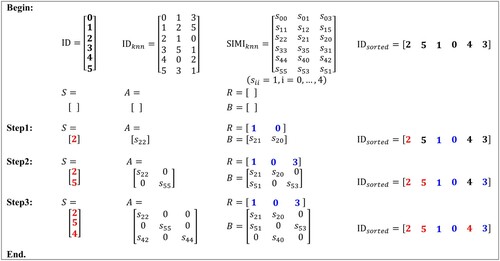
For each point, the KNNS method first calculates the sum of the similarities between it and its $K$-nearest neighbours. The sampling procedure starts by assigning the point with the largest sum, i.e. the one that is most similar to its neighbours. Its neighbours are assigned to the remaining point set directly since they can be considered as representation of the sample. The procedure is repeated until all points in the original data set are assigned. The matrices A and B can be constructed simultaneously during the sampling processing. This cannot be implemented by the MSSS sampling method. The reason for that is when a point is selected as a sample, its neighbours will have no chance to be selected again under the principle of the KNNS method. Figure 5 illustrates the sampling procedure using 2-neighbours as an example. Note that matrix A is asymmetric since the constructed $\mathrm{KNN}$graph is not symmetrical in this design.

Figure 5. Example of the K-nearest neighbour-based sampling (KNNS) method (K = 2). $\mathrm{ID}$ denotes the indices of the points; $\mathrm{I}{\mathrm{D}}_{\mathrm{knn}}$ and $\mathrm{SIM}{\mathrm{I}}_{\mathrm{knn}}$ denote the indices of the $K$-nearest neighbours of each point and the corresponding similarity between them respectively; $\mathrm{I}{\mathrm{D}}_{\mathrm{sorted}}$ is obtained by the sorting $\mathrm{ID}$ according to the descending order of each row sum of $\mathrm{SIM}{\mathrm{I}}_{\mathrm{knn}}$; S is the indices set of sampling points; the set R contains the indices of the remaining points; the matrices $\mathrm{A}$ and $\mathrm{B}$ are defined in 3.1.4.1. The sampling process is performed according to the indices in $\mathrm{I}{\mathrm{D}}_{\mathrm{sorted}}$. Initially, all elements in $\mathrm{I}{\mathrm{D}}_{\mathrm{sorted}}$ are coloured in black, indicating no allocation to S or R. In each step, the first black index in $\mathrm{I}{\mathrm{D}}_{\mathrm{sorted}}$ is put into set S as a new sampling point and is coloured in red. The indices of its $K$-nearest neighbours and the corresponding similarities can be obtained directly in $\mathrm{I}{\mathrm{D}}_{\mathrm{knn}}$ and $\mathrm{SIM}{\mathrm{I}}_{\mathrm{knn}}$. There are three cases for each $K$-nearest neighbour: (a) if it already belongs to S, then put the similarity in the relevant position in A (e.g. $s_{42}$); (b) if it already belongs to R, then put the similarity in the relevant position in B ($\mathrm{e}.\mathrm{g}.s_{51}$,$s_{40}$); (c) if it is neither in S nor R, then add it to R and colour it blue and put the similarity in the relevant position in B (e.g. $s_{53}$). This process ends until there is no black element in $\mathrm{I}{\mathrm{D}}_{\mathrm{sorted}}$.

This method can quickly identify sampling points that satisfy the principle of maximizing the determinant of the sampling similarity matrix mentioned in MSSS. After the construction of the KNN graph, the determinant of the sampling similarity matrix A delivered from KNNS is 1, because A is a lower triangular matrix with the diagonal elements of 1. This is the maximum possible determinant and can minimize the error of the Nyström approximation. Furthermore, our method reduces the computational complexity from the$O(mN)$of the MSSS method to$O(K\cdot N)$, where $K$ represents the number of $K$-nearest neighbours, and $K\ll m$ for a big data set. Another advantage is that the number of samples for the KNNS method is flexible and reliable, since it depends on the structure of the data itself instead of the empirical assumptions.

3.1.5. Individual tree segmentation

After computing the eigenvalues and eigenvectors of the similarity matrix $\hat{W}$, the number of clusters $t$ was chosen by an eigengap heuristic (Luxburg 2007), which is a tool that was particularly designed for spectral clustering. Let ${\lambda }_1,\dots ,{\lambda }_n$ denote the eigenvalues of $\hat{W}$, i.e. the ${\mathrm{\Lambda }}_S$ in Equation (5). The goal is to choose the number t so that all eigenvalues ${\lambda }_1,\dots ,{\lambda }_t$ are very small, and ${\lambda }_{t+1}$ is relatively large. Then, there is a gap between the tth and (t + 1)th eigenvalue, i.e. $|{\lambda }_{t+1}-{\lambda }_t|$ is relatively large. According to the eigengap heuristic, this gap indicates that the data set contains t clusters.

Then, the $k$-means method was applied for the normalized rows of the eigenvector matrix composed of the first t eigenvectors. The clusters of individual trees were obtained by mapping the results back to the original point cloud with reference to the indices of labels. For individual tree parameters, the location and height were defined by the spatial coordinate of the highest point, and the mean of the vertical projections of the clusters in x direction and y direction was taken as the crown radius.

3.1.6. Post-processing

In order to improve the segmentation results, the post-processing workflow was designed as Figure 6. It includes segmentation using NSC method, result merging and filtering, re-segmentation of the filtering points, result filtering and combination of all tested individual trees. The merging and filtering of the segmentation results mainly take into account the distance and height difference of the adjacent trees, the crown shape and the number of points in each tree point cloud. The criteria are as follows:

1. If the distance between two adjacent individual trees is less than the average crown diameter of the corresponding plot and the elevation of these two trees is less than 10 m (10 m here is empirical value through a number of experiments), they will be merged into an individual tree.

2. A tree with a crown diameter greater than half value of the tree height will be empirically regarded as an abnormal crown shape, in view of the fact that it is likely under-segmented. The corresponding tree point cloud will be filtered out so that it can be further searched as potential trees in the re-segmentation.

3. The absolute value of the difference between the East–West crown and the South–North crown is greater than the average of these two values is considered to be an unreasonable result. As the vertical projection of such a canopy usually differs greatly from circle, the corresponding tree point cloud will be filtered out.

Figure 6. Post-processing workflow.

These filtered trees are regarded as unreasonable results obtained by primary segmentation. It is very likely that the filtered points contain potential tree information that was not found. Therefore, the filtered points are re-segmented for further mining point cloud information. And the same filtering process is performed on the re-segmentation results to ensure that the obtained trees are in a reasonable shape. The final segmentation result is the tested individual trees of the primary segmentation and the re-segmentation. In the following, NSC are used to represent the primary results of the Nyström-based Spectral Clustering method.

3.2. Control parameters and sensitivity analysis

There are four parameters that control the performance of the proposed algorithm. The key parameter of the mean shift method is the bandwidth of the kernel function. Since the voxelization is to create local small cells inside each individual tree, we selected the bandwidth based on the local neighbour distance. The average K-nearest neighbour distance was calculated as the bandwidth, where the number of neighbours was determined as the point cloud density. Specifically, the Python sklearn.cluster.estimate_bandwidth function was used to adaptively determine the voxel resolution. Here, the value of the key parameter quantile of the estimate_bandwidth function represents the ratio of the number of neighbours to the number of samples for the nearest neighbour query. In this study, all points in the original cloud were used as samples, and the point density was regarded as an approximate representation of the number of local neighbours overall. Therefore, the ratio of point density and the number of points was calculated and used as the value of quantile parameter. The derived bandwidth value was further used to realize the adaptive mean shift voxelization.

For the width parameters ${\sigma }_{xy}$ and ${\sigma }_z$ of the Gaussian similarity function in Equation (1), i.e. the scale factors for the Euclidean distances, ${\sigma }_z$ was set to six times of ${\sigma }_{xy}$ based on the tree shape in order to make the horizontal and vertical distances the same scale. To find the optimal ${\sigma }_{xy}$, the root mean square of commission costs of the 11 plots in Mengjiagang Forest Farm was considered to evaluate the impact of the parameter. The definition of the commission cost is as follows (Wang et al. 2016) (9) $\mathrm{Commission}\mathrm{Cost}=R_{\mathrm{commission}}/R_{\mathrm{match}}$(9) where the $R_{\mathrm{commission}}$ and $R_{\mathrm{match}}$ are defined by formula (13) and (12) in Section 3.4, respectively. The commission cost is a detection indicator. The lower the value, the higher matching can be obtained. The root mean square of commission costs allows to check the impact of ${\sigma }_{xy}^2$ on the overall detection accuracy and further determine the optimal parameter value. The results of ${\sigma }_{xy}^2$ and the optimal value selection can be found in Section 4.4.

Another important parameter is the number of nearest neighbours in the similarity graph, which is defined as $K$. Since the KNNS method is based on the neighbourhood relationship, different $K$ values will bring different numbers of sampling points in a given voxel space. Thus it will construct the eigenvector matrices with different dimensions. Considering that the number of clusters t is determined by the eigengap heuristic, the dimension of the eigenvector matrix is equal to the upper limit of the number of clusters. Therefore, the value of $K$ ultimately determined the upper limit of the number of final clusters, i.e. the number of trees segmented by the algorithm. To adaptively calculate $K$ in practical application, the relationship between the $K$ values and one of the main attributes of the sampling points, namely the sampling density, was analysed and discussed in Section 4.4.

3.3. Large dataset segmentation

Usually, the airborne LiDAR data covers large area with huge point cloud data volume. Since the computational complexity is $O(n^3)$, when cutting $n$ into multiple sub-blocks $n_1,\dots ,n_p\mathrm{with}{n}_i\ge 0\mathrm{for}i=1,\dots ,p$, it can be drawn that ${\sum }_{i=1}^p{n}_i^3\le n^3$. However, the reprocessing of points near the cutting lines needs to be considered. Excessive cutting may depreciate the first segmentation and result in a heavy burden on reprocessing. Therefore, for tile segmentation, proper cutting can improve efficiency to some extent. In our study, we cut the tile into parts with approximately 300,000 points. The complete tile segmentation process is demonstrated in Figure 7.

Figure 7. The process of tile segmentation. (a) Divide the tile into parts using a cutting line (the blue dashed line); (b) perform the segmentation method in each part to generate individual trees with different labels, and mark the labels near the cutting line in blue; (c) gather the points with blue labels (the grey points with label 0), and merge other labels in order (labels 3–5 below were updated to 4–6 to follow the upper label 1–3); (d) re-segment the grey points and merge their labels to the final results.

3.4. Accuracy assessment

The accuracy of the algorithm was assessed in terms of both detection rates and tree parameters. The matching method proposed by Eysn et al. (2015) was performed, which mainly based on tree height and horizontal distance. Figure 8 illustrates an example of the matching process for one reference tree. The whole procedure started from the highest detected tree, and searched for the reference trees that satisfied the height and distance criterion in Table 4 as match candidates. If a farther candidate showed a better height difference (ΔH) and its 2D distance between detection and reference (ΔD) was at a maximum of 2.5 m greater than the nearer one, then it became a better match. This process was repeated until all detected trees have been checked. Finally, the matched reference trees were checked against the surrounding detection trees. If the closest one with the smallest height difference is the matched detection tree previously, these two trees will be treated as a matched pair. Otherwise, the matched reference tree will be removed.

Figure 8. Matching procedure for a reference tree with height of 20 m. Here, the number represents the tree height. (a) The detected trees that are not within the distance criterion of the reference are removed (19 and 23 m). Here, the criterion is ΔD < 5 m since 15 m < H = 20 m ≤ 25 m. (b) The detected trees that do not satisfy the height criterion in Table 3 are removed (12 m). Here, the criterion is ΔH < 4 m. (c) The detection with 21 m height became the best match since it shows a better ΔH and its distance from the reference (2.2 m) is 0.7 m (<2.5 m) greater than the near detection with 17 m height (1.5 m).

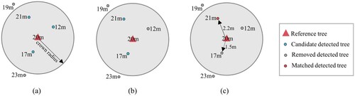
Table 4. Criterions of tree height and 2D distance for the matching procedure (Eysn et al. 2015).

No.	Tree height	Height criterion	Distance criterion
1	H ≤ 10 m	ΔH < 3 m	ΔD < 3 m
2	10 m < H ≤ 15 m	ΔH < 3 m	ΔD < 4 m
3	15 m < H ≤ 25 m	ΔH < 4 m	ΔD < 5 m
4	H > 25 m	ΔH < 5 m	ΔD < 5 m

For a dataset with high stem density, several candidates may be searched using the distance criterion in Table 4. This phenomenon results in several more distant candidates initially becoming matches, and these matches are very likely to be removed when the references are final checked. In order to check the effect of the matching methods, we also matched the detection results using the crown radius as an adaptive distance criterion instead of the fixed threshold. Considering the insufficient positioning accuracy of the stems (Section 2.1), a constant value of 1 m is added to the crown radius.

According to the matching procedure above, the segmentation results can be divided into $\mathrm{TP}$ (true positive), $\mathrm{FN}$ (false negative) and $\mathrm{FP}$ (false positive), representing the match, omission and commission, respectively, where $\mathrm{TP}+\mathrm{FN}=N_{\mathrm{reference}}$ and $\mathrm{TP}+\mathrm{FP}=N_{\mathrm{detection}}$. The extraction rate ($R_{\mathrm{extraction}}$), matching rate ($R_{\mathrm{match}}$) and commission rate ($R_{\mathrm{commission}}$) can be calculated by (10) $R_{\mathrm{extraction}}={\displaystyle \frac{N_{\mathrm{detection}}}{N_{\mathrm{reference}}}={\displaystyle \frac{\mathrm{TP}+\mathrm{FP}}{\mathrm{TP}+\mathrm{FN}}}}$(10) (11) $R_{\mathrm{match}}={\displaystyle \frac{N_{\mathrm{match}}}{N_{\mathrm{reference}}}={\displaystyle \frac{\mathrm{TP}}{\mathrm{TP}+\mathrm{FN}}}}$(11) (12) $R_{\mathrm{commission}}={\displaystyle \frac{N_{\mathrm{commission}}}{N_{\mathrm{detection}}}={\displaystyle \frac{\mathrm{FP}}{\mathrm{TP}+\mathrm{FP}}=1-{\displaystyle \frac{R_{\mathrm{match}}}{R_{\mathrm{extraction}}}}}}$(12) (13) $R^2={\displaystyle \frac{{\sum }_{i=1}^n(H_i-\overline{H_i})(\widehat{H_i}-\overline{\widehat{H_i}})}{\sqrt{{\sum }_{i=1}^n{(H_i-\overline{H_i})}^2}\sqrt{{\sum }_{i=1}^n{(\widehat{H_i}-\overline{\widehat{H_i}})}^2}}}$(13) (14) $\mathrm{RMSE}=\sqrt{\sum _{i=1}^n{(H_i-\widehat{H_i})}^2}$(14) (15) $\mathrm{rRMSE}={\displaystyle \frac{\mathrm{RMSE}}{\overline{\widehat{W_i}}}}$(15)

In order to estimate the segmentation performance, the R-squared measure ($R^2$), root mean square error ($\mathrm{RMSE}$) and relative root mean square error (rRMSE) of tree height regression were calculated. The calculation methods of these parameters are shown in formulas (13)–(15).$H_i$ is tree height from reference, $\overline{H_i}$ is the average of $H_i$, $\widehat{H_i}$ is tree height from detection, $\overline{\widehat{H_i}}$ is the average of $\widehat{H_i}$, n is the number of trees.

For the tile segmentation, the results were assessed by the plots within it. Considering the field data characteristics in Section 2.1, the tree height were evaluated using the field plots from #1 to # 11 in Mengjiagang and the field plots from #13 to #18 in Dagujia, which have field measured tree height for all the tally trees and selected trees. As the tree heights in plot #12 were estimated using DBH, we did not use these plots for the height evaluation. The extraction rate and matching rate were evaluated using field plots from #1 to #12, which have field measured stem positions. As only a part of stem positions were measured for plots from #13 to #18 in Dagujia, these plots were not used for extraction rate and matching rate evaluation.

4. Results

4.1. Individual tree segmentation

Figure 9 shows the segmentation results with different stem densities. Relative to the field-measured data, the best results were obtained for low stem density (Figure 9(a)). The segmentation for a small tree covered by a large tree is quite difficult, for example the small referenced tree in Figure 9(c). It is mainly because there is fewer airborne LiDAR point data in this situation. Figure 10 visually displays the detection rates of 11 standard plots and 1 large plot using the crown radius and distance criterion for matching procedure. Compared with distance criterion, the matching method using crown radius has a lower matching rate of each plot because of its rigorous matching rules, especially for the medium and high stem densities.

Figure 9. Examples of segmentation results for different stem densities. Each colour represents one segmented tree, and the black points are the stem positions of field-measured data with different height represents the inventory tree height. (a) Low stem density, (b) medium stem density, and (c) high stem density.

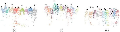
Figure 10. Extraction rates and matching rates for different forest plots. The annotations ‘match_cr’ and ‘match_dc’ represent the matching procedure using crown radius and distance criterion, respectively.

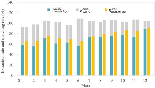
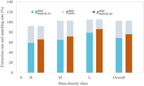
For NSC method, Figure 11 shows that the matching rates increase from 54% to 74% (crown radius for matching procedure) as stem density decreases. The lowest extraction rate is found in the medium stem density plot ($R_{\mathrm{extr}.}^{\mathrm{NSC}}$: 102%), which was almost consistent with the overall performance. The matching procedure using crown criterion obtained lower matching rates with 8%, 7% and 7% lower than the matching procedure using distance radius for high, medium and low stem density plots respectively. Overall, NSC algorithm extracted 103% of the reference trees, 70% of which were correctly matched using distance criterion for matching procedure, and 65% of which were correctly matched using crown radius for matching procedure.

Figure 11. Extraction rates and matching rates for different stem density levels. The annotations ‘match_cr’ and ‘match_dc’ represent the matching procedure using crown radius and distance criterion, respectively.

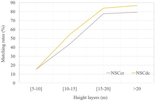
To observe the performance of the algorithm, we further examined the results by different tree height levels (Figure 12). Considering the matching rates using crown radius, the best matching rate was obtained as 79% in the layer >20 m for NSC method. The matching rate for the layer 5–20 m is 78% which is also a relatively better result. For the layer 10–15 m and the layer 5–10 m, the matching rates are 44% and 15%. The matching rates are 15%, 54%, 84% and 87% when using distance criterion for the layer 5–10 m, 10–15 m, 15–20 m and >20 m. All are higher than the results obtained by the matching method using crown radius.

Figure 12. Extraction rates and matching rates for different tree height levels. The annotations ‘cr’ and ‘dc’ represent the matching procedure using crown radius and distance criterion, respectively.

4.2. Tree height accuracy evaluation

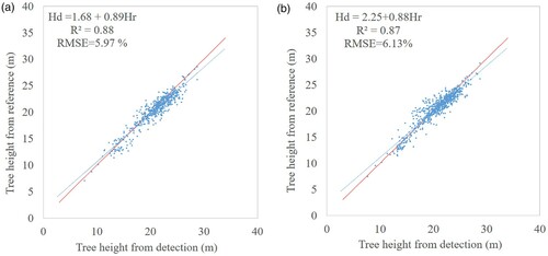
High tree height accuracy was found for the tree parameters of the matches (Figure 13). The large plot 12 was excluded because of its insufficient accuracy of the reference height of each stem which were obtained from empirical model rather than measured value. As shown in Figure 13, the $R^2$ value is 0.87 and the RMSE value is 1.26 m with rRMSE of 6.13% for the matching procedure using distance criterion. The matching procedure using crown radius obtained better results with a higher $R^2$ value of $0.88\mathrm{and}\mathrm{a}\mathrm{lower}\mathrm{RMSE}\mathrm{values}\mathrm{of}1.22\mathrm{m}\mathrm{with}\mathrm{rRMSE}\mathrm{of}5.97\text{\%}$.

Figure 13. Precision of tree height of plots 1–11. (a) For NSC method using crown radius in matching procedure, (b) for NSC method using distance criterion in matching procedure.

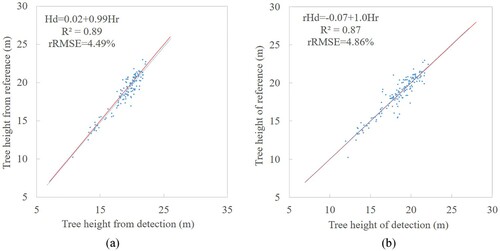
Furthermore, different matching procedures were also used to match the height of detected trees with the reference stems positioned by total station in the 13–18 plots (Figure 14). Compared with the tree position measured by tape and RTK, there are more accurate stem locations obtained by total station which show better results in the tree height matching. For the matching procedure using distance criterion, the $R^2$ is 0.87 and the RMSE is 0.90 m with rRMSE of 4.86%. The matching procedure using crown radius obtained better results with the $R^2$ of 0.89, RMSE of 0.84 m and rRMSE of 4.49%. And the estimated tree height is very close to field measured height.

Figure 14. Precision of tree height of plots 13–18. (a) For NSC method using crown radius in matching procedure, (b) for NSC method using distance criterion in matching procedure.

4.3. Comparison of plot- and tile-scale segmentation

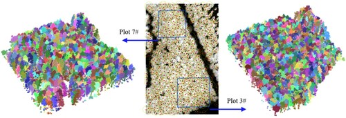
For the tile segmentation (the testing tile in Figure 1), total 37,160 trees are obtained. Figure 15 shows the segmentation results of the three plots in plot scale and tile scale, which keeps almost the same height distribution. Figure 16 compares the results of the three plots at different height scales to view the accuracy of the algorithm in tile segmentation. Overall, the matching rate and parameter precision are almost the same at plot and tile scales. Even the plot scale can obtain a slightly higher matching rates compared with the tile scale. It implies that our algorithm is independent of scale, and can perform well for large-scale LiDAR point cloud data. Figure 17 shows segmentation results of 3# and 7# sample plot in tile scale.

Figure 15. Height distribution of the segmentation results for the three plots at plot scale and tile scale.

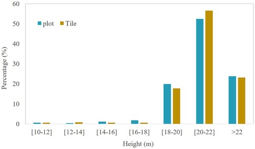
Figure 16. Comparison of tile and plot segmentation results. The annotations ‘NSC’ represent the proposed method. The annotations ‘cr’ and ‘dc’ represent the matching procedure using crown radius and distance criterion. The annotations ‘Plot’ and ‘Tile’ represent the results in plot and tile scale.

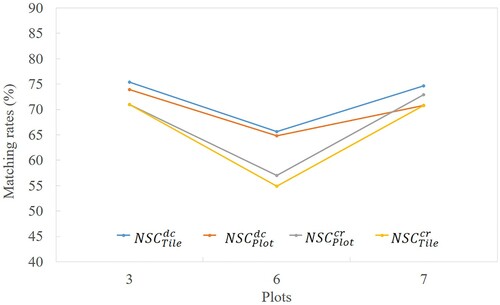
Figure 17. Segmentation results of the 3# and 7# plots in tile scale. The raster image is part of the CHM of the tile shown in Figure 1, which includes the 3# and 7# sample plots. The red triangles are the position of the individual trees after segmentation, and the yellow circles indicate the crown width of the trees. Two large blue boxes represent the extent of the 3# and 7# sample plots. The point cloud shows the final segmentation results of the two plots, and different colours represent different individual trees.

4.4. Comparison with other segmentation methods

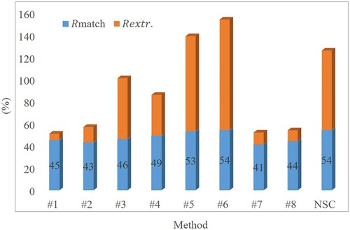
The direct comparison results with other methods using the benchmark dataset are shown in Figure 18. The descriptions of methods #1–#8 can be found in Eysn et al. (2015). Compared with other 8 methods, the matching rate of the proposed NSC method ($\mathrm{RM}{\mathrm{S}}_{\mathrm{match}}$: 54%) is higher than the other methods. Meanwhile, although methods #5 and #6 have similar matching rates with the proposed NSC method, they have much larger extraction rate, which means these two methods have very high risk of commission errors.

Figure 18. Detection results of different segmentation methods using benchmark dataset in the Alpine Space of Europe. #1–#8 correspond to the methods described by Eysn et al. (2015). NSC represents the proposed method.

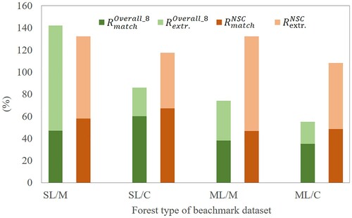
In Figure 19, the detection results are summarized by forest type. This comparison was only conducted with the overall results of other eight methods because only the quantitative value of the overall accuracy is available in the work of Eysn et al. (2015). The best result of NSC method was found for single-layered mixed forests (SL/M), showing a lower $\mathrm{RM}{\mathrm{S}}_{\mathrm{extr}.}$ (132%) and a higher $\mathrm{RM}{\mathrm{S}}_{\mathrm{match}}$ (58%) than those values of other 8 methods. The performance for single-layered coniferous forests (SL/C) is also satisfactory, with a better $\mathrm{RM}{\mathrm{S}}_{\mathrm{match}}$ (67%) and a worse $\mathrm{RM}{\mathrm{S}}_{\mathrm{extr}.}$ (117%). The multi-layered mixed forests (ML/M) and multi-layered coniferous forests (ML/C) show similar results with higher extraction rates, while the $\mathrm{RM}{\mathrm{S}}_{\mathrm{match}}$ values are 8% and 13% higher than those values of other eight methods.

Figure 19. Detection results by forest type of different segmentation methods using benchmark dataset in the Alpine Space of Europe. Overall_8 represents the overall result of other eight methods. The forest class corresponds to single or multi-layered (SL or ML)/mixed or coniferous (M or C).

4.5. Parameter sensitivity

Figures 20 and 21 show the results of sensitivity analysis using the 11 plots in Mengjiagang Forest Farm. Regarding the width parameters ${\sigma }_{xy}$ of the Gaussian similarity function in equation (1)(1) $s(x_i,x_j)=\{\begin{array}{cc}{e}^{-n_i{n}_j{\left({\displaystyle \frac{D_{ij}^{XY}}{{\sigma }_{xy}}}\right)}^2}\times e^{-n_i{n}_j{\left({\displaystyle \frac{D_{ij}^Z}{{\sigma }_z}}\right)}^2}& \mathrm{if}(x_j\mathrm{in}\mathrm{KNN}\mathrm{of}{x}_i)\\ 0& \mathrm{otherwise}\end{array}$(1) , Figure 20 shows the root mean square value of the commission cost when varying the values of ${\sigma }_{xy}^2$, and the optimal choice is ${\sigma }_{xy}^2=10{\mathrm{m}}^2$, i.e. ${\sigma }_{xy}\approx 3.16\mathrm{m}$. Accordingly, ${\sigma }_z$ is taken as 18.96 m. 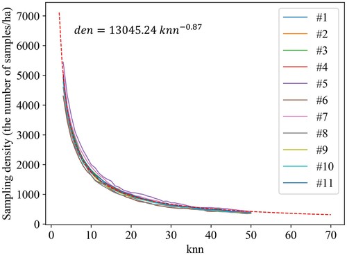With respect to the value of $K$ in the similarity graph, Figure 21 shows the changes of sampling density values of the 11 plots in Mengjiagang when varying the $K$ from 3 to 50. Regardless of the characteristics of plots, there is a fixed relationship between the value of $K$ and the density of the sampling points (the red dotted line in Figure 21). The detail is as follows: (16) $\mathrm{den}=13,045.24K^{-0.87}$(16) where $\mathrm{den}$ (num/ha) represents the density of the sampling points, $K$ denotes the number of nearest neighbour in the KNN method. The main attributes of the point cloud data considered are the point density and plot area. The voxelization process removed the former effect using the bandwidth determined by the point density. The density of the sampling points, an area-independent attribute, eliminated the effect of the plot area. In practical application, the values of $\mathrm{den}$ can be calculated based on the number of local maxima in the CHM. Then the values of $K$ can be adaptively obtained by equation (16)(16) $\mathrm{den}=13,045.24K^{-0.87}$(16) .

Figure 20. Influence of ${\sigma }_{xy}^2$ on the values of root mean square of commission cost for the 11 plots in Mengjiagang Forest Farm. The optimal value (red dot) appears near ${\sigma }_{xy}^2=10{\mathrm{m}}^2$.

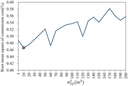
Figure 21. Influence of $K$ (the number of neighbours) on the values of $\mathrm{den}$ (the density of the sampling points) for the 11 plots in Mengjiagang Forest Farm.

5. Discussion

5.1. Voxel weights for the similarity function

The voxel weights introduced in the similarity function have an important influence on the algorithm. In the comparison of Table 5, voxel weights produced better matching rates both in the overall results and in every stem density class for each matching method. Although the matching method using crown radius has lower matching rates, it can obtain higher precision of tree height.

Table 5. Comparison of the segmentation results for different similarity functions using different matching methods.

Matching method	Segmentation method	$R_{\mathrm{match}}$ (%)	$R_{\mathrm{match}}$_H (%)	$R_{\mathrm{match}}$_M (%)	$R_{\mathrm{match}}$_L (%)	Tree height
						$R^2$	$\mathrm{RMSE}$ (m)
Distance criterion	$\mathrm{NS}{\mathrm{C}}_0$	62	53	55	75	0.87	1.36
	$\mathrm{NS}{\mathrm{C}}_{\mathrm{vw}}$	74	66	70	84	0.87	1.26
Crown radius	$\mathrm{NS}{\mathrm{C}}_0$	54	46	48	69	0.87	1.28
	$\mathrm{NS}{\mathrm{C}}_{\mathrm{vw}}$	67	58	63	78	0.88	1.22

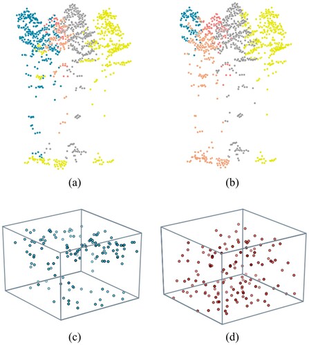
Figure 22 illustrates the reason for the improvement by introducing voxel weights in the similarity function. The similarity function without voxel weights produced unconnected clusters, such as the abnormal individuals coloured in yellow in Figure 22(a). The distributions of the sampling points generated by different similarity functions reveal the essence of this problem (Figure 22(c,d)). The density-based voxelization results in a few but heavy voxels in dense local areas. If the weights are neglected, these areas will become sparse in the voxel cloud (the nonuniform distribution in Figure 22(c)). For the sampling process based on the neighbour relationship, these remote but representative voxels will not be remained, as they can be represented by other light but dense samples. Such unreasonable sampling (Figure 22(c)) leads to the problem in Figure 22(a). On the contrary, voxel weights produce reasonable sampling results (the uniform distribution in Figure 22(d)) and thus eliminate the disconnection (Figure 22(b)).

Figure 22. Segmentation results for the same part of plot 11 produced by (a) the similarity function without voxel weights, occurring an unconnected individual (the yellow cluster), and (b) the similarity function with voxel weights, producing no abnormal cluster. Different colours represent different segmented trees. (c) and (d) are the sampling points generated in plot 11 using the similarity function without and with voxel weights, respectively. Here, the grey cube represents the boundary of the plot.

5.2. Comparison of different sampling methods

Table 5 compares the detection results of different sampling methods of the plots #1–#12 using different matching methods. Due to the random characteristic of the MSSS method (Bouneffouf and Birol 2015), fixed parameters can also produce various outcomes. The results presented here are optimal for multiple experiments. The quantitative comparison in Table 6 shows that KNNS obtained higher matching rates not only in the overall results but also in different stem density classes for every matching method. The matching tree parameters of the two methods are approximately the same for a certain matching method. In addition, the KNNS method can achieve more stable results with faster calculation (Section 3.1.4.2). Hence this method is more feasible in practical applications.

Table 6. Comparison of the segmentation results for different sampling methods using different matching methods.

Matching method	Segmentation method	$\mathrm{RM}{\mathrm{S}}_{\mathrm{match}}$ (%)	$\mathrm{RM}{\mathrm{S}}_{\mathrm{match}}$_H (%)	$\mathrm{RM}{\mathrm{S}}_{\mathrm{match}}$_M (%)	$\mathrm{RM}{\mathrm{S}}_{\mathrm{match}}$_L (%)	Tree height
						$R^2$	$\mathrm{RMSE}$ (m)
Distance criterion	$\mathrm{NS}{\mathrm{C}}_{\mathrm{MSSS}}$	71	66	66	82	0.87	1.44
	$\mathrm{NS}{\mathrm{C}}_{\mathrm{KNNS}}$	74	66	70	84	0.87	1.26
Crown radius	$\mathrm{NS}{\mathrm{C}}_{\mathrm{MSSS}}$	64	54	61	70	0.89	1.31
	$\mathrm{NS}{\mathrm{C}}_{\mathrm{KNNS}}$	67	58	63	78	0.88	1.22

5.3. Effects of matching methods

The matching method using crown radius can improve the tree height precision at the cost of a small reduction in matching rates in comparison with the matching method using distance criterion (Figures 13 and 14), especially in the plots with medium and high density. The problem is mainly due to the fact that the fixed threshold of Table 4 might be too large for high stem density plots. It could search many candidates especially when the commission rate is relatively high. In the final check of the reference, the farther matched candidates are likely to be filtered out. The crown radius can get more reasonable match trees compared with the distance criterion, but a match may not be searched in a more rigorous range of crown radius which results in the lower matching rates. The matched trees in the range of crown radius are the most reasonable results, and the accuracy of the tree height can be approved. In addition, the insufficient accuracy of the field stem position may be another reason of lower matching rates using crown radius. It can be inferred that more satisfactory results could be expected with higher accurate field single stem positioning.

6. Conclusions

This study developed a new individual tree segmentation method based on airborne LiDAR point cloud data directly. We used the mean shift voxelization and Nyström approximation for the spectral clustering method to isolate individual trees. By using the similarity graph with voxel weight and the K-nearest neighbour-based sampling (KNNS) scheme, the proposed algorithm not only reduced the storage and calculation complexity of the spectral clustering algorithm but also maintain its good segmentation performance. In the study sites with various levels of LiDAR point density and tree stem density, our algorithm extracted 103% of the reference trees, 69% of which were correctly matched using crown radius criterion. The matching method using crown radius is a more adaptive choice than distance criterion because it provides more reasonable linkage, especially for the high stem density plots. For all trees from 11 plots with GNSS calibrated tape-measured locations in Mengjiagang Forest Farm, the tree height regression of the matching results shown an $R^2$ of 0.88 and a $RMSE$ of 1.22 m. For all trees from 6 plots with GNSS calibrated total-station measured locations in Dagujia Forest Farm, the $R^2$ and $RMSE$ values of tree height regression reached 0.89 and 0.84 m. The consistence between plot and tile segmentation indicates that the algorithm can provide stable and favourable results for large-scale airborne LiDAR data. In comparison with other sampling methods using a benchmark dataset, the proposed KNNS method also shows better performance. Moreover, the introduction of voxel weights in the similarity function effectively solved the problem of abnormal clustering.

Disclosure statement

No potential conflict of interest was reported by the author(s).

Data availability statement

The relevant code of this research is available at https://github.com/limingado/NSC/tree/v1.0.0.

Additional information

Funding

This study was funded by the National Key Research and Development Program of China [grant number 2017YFD0600404] and Natural Science Foundation of China [grant number 41871278].

Notes

Note: The stem density classes correspond to high (H), medium (M) and low (L) levels.

^a Only selected trees with total station location are included for these plots.

Note: Corresponding Latin names: spruce (Picea abies), fir (Abies alba), beech (Fagus sylvatica), Scots pine (Pinus sylvestris), larch (Larix decidua), sycamore (Acer pseudoplatanus), elm (Ulmus glabra), and poplar (Populus nigra). These plots include forests of single or multi-layered (SL or ML)/mixed or coniferous (M or C).

Note: ΔH and ΔD represent the height difference and 2D distance between detection and reference.

Note: $\mathrm{NS}{\mathrm{C}}_{\mathrm{vw}}$ and $\mathrm{NS}{\mathrm{C}}_0$ represent the Nyström-based spectral clustering with and without the voxel weights in the similarity function. $R_{\mathrm{match}}$ represents the overall performance and the $R_{\mathrm{match}}$ with H, M, L correspond to the stem density class in Table 1.

References

- Ayrey, E., S. Fraver, J. A. Kershaw Jr, L. S. Kenefic, D. Hayes, A. R. Weiskittel, and B. E. Roth. 2017. “Layer Stacking: A Novel Algorithm for Individual Forest Tree Segmentation from LiDAR Point Clouds.” Canadian Journal of Remote Sensing 43 (1): 16–27. doi:https://doi.org/10.1080/07038992.2017.1252907.
- Bouneffouf, D., and I. Birol. 2015. “Sampling with Minimum Sum of Squared Similarities for Nystrom-Based Large Scale Spectral Clustering.” Paper presented at the International Conference on Artificial Intelligence, January 25–29. AAAI Press.
- Brandtberg, T., T. A. Warner, R. E. Landenberger, and J. B. McGraw. 2003. “Detection and Analysis of Individual Leaf-off Tree Crowns in Small Footprint, High Sampling Density Lidar Data from the Eastern Deciduous Forest in North America.” Remote Sensing of Environment 85 (3): 290–303. doi:https://doi.org/10.1016/S0034-4257(03)00008-7.
- Chen, Q., D. Baldocchi, P. Gong, and M. Kelly. 2006. “Isolating Individual Trees in a Savanna Woodland Using Small Footprint Lidar Data.” Photogrammetric Engineering & Remote Sensing 72 (8): 923–932. doi:https://doi.org/10.14358/PERS.72.8.923.
- Cohen, M. B., Y. T. Lee, C. Musco, C. Musco, R. Peng, and A. Sidford. 2015. “Uniform Sampling for Matrix Approximation.” In Proceedings of the 2015 Conference on Innovations in Theoretical Computer Science, January 11–13, 181–190. doi:https://doi.org/10.1145/2688073.2688113.
- Eysn, L., M. Hollaus, E. Lindberg, F. Berger, J. M. Monnet, M. Dalponte, M. Pellegrini, et al. 2015. “A Benchmark of Lidar-Based Single Tree Detection Methods Using Heterogeneous Forest Data from the Alpine Space.” Forests 6 (5): 1721–1747. doi:https://doi.org/10.3390/f6051721.
- Fowlkes, C., S. Belongie, F. Chung, and J. Malik. 2004. “Spectral Grouping Using the Nystrom Method.” IEEE Transactions on Pattern Analysis and Machine Intelligence 26 (2): 214–225. doi:https://doi.org/10.1109/TPAMI.2004.1262185.
- Gupta, S., H. Weinacker, and B. Koch. 2010. “Comparative Analysis of Clustering-Based Approaches for 3-D Single Tree Detection Using Airborne Fullwave Lidar Data.” Remote Sensing 2 (4): 968–989. doi:https://doi.org/10.3390/rs2040968.
- Heinzel, J., and M. O. Huber. 2018. “Constrained Spectral Clustering of Individual Trees in Dense Forest Using Terrestrial Laser Scanning Data.” Remote Sensing 10 (7), Article number 1056. doi:https://doi.org/10.3390/rs10071056.
- Hyyppä, J., H. Hyyppä, M. Inkinen, M. Engdahl, S. Linko, and Y. H. Zhu. 2000. “Accuracy Comparison of Various Remote Sensing Data Sources in the Retrieval of Forest Stand Attributes.” Forest Ecology and Management 128 (1-2): 109–120. doi:https://doi.org/10.1016/s0378-1127(99)00278-9.
- Lee, H., K. C. Slatton, B. E. Roth, and W. P. Cropper Jr. 2010. “Adaptive Clustering of Airborne LiDAR Data to Segment Individual Tree Crowns in Managed Pine Forests.” International Journal of Remote Sensing 31 (1): 117–139. doi:https://doi.org/10.1080/01431160902882561.
- Li, M. L., and C. M. Sun. 2018. “Refinement of LiDAR Point Clouds Using a Super Voxel Based Approach.” ISPRS Journal of Photogrammetry and Remote Sensing 143: 213–221. doi:https://doi.org/10.1016/j.isprsjprs.2018.03.010.
- Liang, X. J., Y. Pang, and B. W. Chen. 2020. “Accurate Measurement of Individual Tree Position Based on DBH Extraction of Terrestrial Laser Scanning.” Forest Research 33 (4): 67–74. doi:https://doi.org/10.13275/j.cnki.lykxyj.2020.04.009.
- Lin, F., and W. W. Cohen. 2010. “Power Iteration Clustering.” In Proceedings of the 27th International Conference on Machine Learning (ICML-10), June 21–24.
- Lindberg, E., and J. Holmgren. 2017. “Individual Tree Crown Methods for 3D Data from Remote Sensing.” Current Forestry Reports 3 (1): 19–31. doi:https://doi.org/10.1007/s40725-017-0051-6.
- Luxburg, U. V. 2007. “A Tutorial on Spectral Clustering.” Statistics and Computing 17 (4): 395–416. doi:https://doi.org/10.1007/s11222-007-9033-z.
- Morsdorf, F., E. Meier, B. Kötz, K. I. Itten, M. Dobbertin, and B. Allgöwer. 2004. “LiDAR-Based Geometric Reconstruction of Boreal Type Forest Stands at Single Tree Level for Forest and Wildland Fire Management.” Remote Sensing of Environment 92 (3): 353–362. doi:https://doi.org/10.1016/j.rse.2004.05.013.
- Pang, Y., Z. Y. Li, H. B. Ju, H. Lu, W. Jia, L. Si, Y. Guo, et al. 2016. “LiCHy: The CAF’s LiDAR, CCD and Hyperspectral Integrated Airborne Observation System.” Remote Sensing 8 (5), Article number 398. doi:https://doi.org/10.3390/rs8050398.
- Popescu, S. C., R. H. Wynne, and R. F. Nelson. 2002. “Estimating Plot-Level Tree Heights with Lidar: Local Filtering with a Canopy-Height Based Variable Window Size.” Computers and Electronics in Agriculture 37 (2002): 71–95. doi:https://doi.org/10.1016/S0168-1699(02)00121-7.
- Reitberger, J., C. Schnörr, P. Krzystek, and U. Stilla. 2009. “3D Segmentation of Single Trees Exploiting Full Waveform LiDAR Data.” ISPRS Journal of Photogrammetry and Remote Sensing 64 (2009): 561–574. doi:https://doi.org/10.1016/j.isprsjprs.2009.04.002.
- Sačkov, I., T. Hlásny, T. Bucha, and M. Juriš. 2017. “Integration of Tree Allometry Rules to Treetops Detection and Tree Crowns Delineation Using Airborne Lidar Data.” iForest-Biogeosciences and Forestry 10 (2): 459–467. doi:https://doi.org/10.3832/ifor2093-010.
- Shi, J. B., and J. Malik. 2000. “Normalized Cuts and Image Segmentation.” IEEE Transactions on Pattern Analysis and Machine Intelligence 22 (8): 888–905. doi:https://doi.org/10.1109/34.868688.
- Sloan, I. H. 1981. “Quadrature Methods for Integral Equations of the Second Kind over Infinite Intervals.” Mathematics of Computation 36 (1981): 511–523. doi:https://doi.org/10.1090/S0025-5718-1981-0606510-2.
- Wang, Y. S., J. Hyyppä, X. L. Liang, H. Kaartinen, X. W. Yu, E. Lindberg, J. Holmgren, et al. 2016. “International Benchmarking of the Individual Tree Detection Methods for Modeling 3-D Canopy Structure for Silviculture and Forest Ecology Using Airborne Laser Scanning.” IEEE Transactions on Geoscience and Remote Sensing 54 (9): 5011–5027. doi:https://doi.org/10.1109/TGRS.2016.2543225.
- Williams, J., C. B. Schonlieb, T. Swinfield, J. Lee, X. H. Cai, L. Qie, and D. A. Coomes. 2020. “3D Segmentation of Trees Through a Flexible Multiclass Graph Cut Algorithm.” IEEE Transactions on Geoscience and Remote Sensing 58 (2): 754–776. doi:https://doi.org/10.1109/TGRS.2019.2940146.
- Yao, W., P. Krzystek, and M. Heurich. 2012. “Tree Species Classification and Estimation of Stem Volume and DBH Based on Single Tree Extraction by Exploiting Airborne Full-Waveform LiDAR Data.” Remote Sensing of Environment 123 (2012): 368–380. doi:https://doi.org/10.1016/j.rse.2012.03.027.
- Ye, W., S. Goebl, C. Plant, and C. Böhm. 2016. “Fuse: Full Spectral Clustering.” In Proceedings of the 22nd ACM SIGKDD International Conference on Knowledge Discovery and Data Mining, August 13–17, 1985–1994. doi:https://doi.org/10.1145/2939672.2939845.
- Zeng, Z. C., M. Zhu, H. Yu, and H. L. Ma. 2014. “Minimum Similarity Sampling Scheme for Nyström Based Spectral Clustering on Large Scale High-Dimensional Data.” In International Conference on Industrial, Engineering and Other Applications of Applied Intelligent Systems, July 10–11, 260–269. doi:https://doi.org/10.1007/978-3-319-07467-2_28.
- Zhang, K., I. W. Tsang, and J. T. Kwok. 2008. “Improved Nyström Low-Rank Approximation and Error Analysis.” In Proceedings of the 25th International Conference on Machine Learning, July 5, 1232–1239. doi:https://doi.org/10.1145/1390156.1390311.
- Zhang, X., and Q. You. 2011. “Clusterability Analysis and Incremental Sampling for Nyström Extension Based Spectral Clustering.” In 2011 IEEE 11th International Conference on Data Mining, December 11–14, 942–951. doi:https://doi.org/10.1109/ICDM.2011.35.
- Zhao, D., Y. Pang, Z. Y. Li, and L. J. Liu. 2014. “Isolating Individual Trees in a Closed Coniferous Forest Using Small Footprint Lidar Data.” International Journal of Remote Sensing 35 (20): 7199–7218. doi:https://doi.org/10.1080/01431161.2014.967886.
- Zimble, D. A., D. L. Evans, G. C. Carlson, R. C. Parker, S. C. Grado, and P. D. Gerard. 2003. “Characterizing Vertical Forest Structure Using Small-Footprint Airborne LiDAR.” Remote Sensing of Environment 87 (2003): 171–182. doi:https://doi.org/10.1016/S0034-4257(03)00139-1.