Understanding temporal stability: a long-term analysis of USDA ARS watersheds

ABSTRACT

The U.S. Department of Agriculture’s Agricultural Research Service (USDA-ARS) maintains seven in situ soil moisture networks throughout the continental United States, some since 2002. These networks are crucial for understanding the spatial and temporal extent of droughts in their historical context, parameterization of hydrologic models, and local agricultural decision support. However, the estimates from these networks are dependent upon their ability to provide reliable soil moisture information at a large scale. It is also not known how many network stations are sufficient to monitor watershed scale dynamics. Therefore, the objectives of this research were to: (1) determine how temporally stable these networks are, including the relationships between various sensors on a year-to-year and seasonal basis, and (2) attempt to determine how many sensors are required, within a network, to approximate the full network average. Using data from seven in situ, it is concluded that approximately 12 soil moisture sensors are sufficient in most environments, presuming their locations are distributed to capture the hydrologic heterogeneity of the watershed. It is possible to install a temporary network containing a suitable number of sensors for an appropriate length of time, glean stable relationships between locations, and retain these insights moving forward with fewer sensor resources.

KEYWORDS:

• Soil moisture
• temporal stability
• in situ networks

1. Introduction

In situ soil moisture networks play a pivotal role in understanding watershed scale soil moisture dynamics. Hydrologic models frequently employ estimates of subsurface flows at the watershed scale. To generate these estimates, it is necessary to have time series data for soil moisture (e.g. Grayson et al. 1997; Bell, Weng, and Luo 2010). Soil moisture products are deployed for applications from agricultural decision support regarding field trafficability (Coopersmith et al. 2014), to the Department of Defense (Jones et al. 2010). Long-term climate assessments, made with General Circulation Models (GCMs), to mitigate sources of uncertainty, necessitate inputs of soil moisture (e.g. Koster and Milly 1997; Belair et al. 2005; De Rosnay et al. 2013; Campoy et al. 2013; Joetzjer et al. 2013). Analyzes of drought events at multiple spatial and temporal scales also contain soil moisture data as a prerequisite input (Sheffield et al. 2004). Each of these applications requires accurate and reliable soil moisture information over sufficiently long time scales.

It is beneficial to understand if the relative wetness/dryness of the installed sensors is temporally stable on a year-to-year basis. This type of analysis was initiated by Vachaud et al. (1985) which analyzed a number of soil moisture monitoring sites and ranked their relative average moisture status. Starks et al. (2006) applied this to a watershed scale network with soil moisture profiles and found. Cosh et al. (2006, 2014) addressed spatial distributions of soil moisture across watershed scales in Oklahoma which cover different landscapes in Oklahoma. These studies found that surface soil moisture patterns were stable, but didn’t necessarily translate through the soil profile. Remote sensing validation using networks has been done in a variety of ways, including Martinez-Fernandez and Ceballos (2005) for the REMEDHUS network in Spain which found that one year of data was sufficient for the determination of mean soil moisture. However, this study was based on two networks in the same River Duero basin in Spain with approximately four years of data each which may not be sufficient for long-term studies. These studies calculated the stability of ordinal rankings of sensors within watershed networks reveals whether or not it is plausible to replace a ‘missing’ reading for a given hour with an estimate that is appropriately wetter or drier than the remaining network average. In addition to the need for understanding inter-annual temporal stability, understanding seasonal temporal stability is also important. In other words, are those sensors that are wettest/driest in April the same sensors that are wettest/driest in July/October?

Once we have established the stability of seasonal and inter-annual rankings of sensor wetness within a given watershed, we can determine how many sensors are required to characterize a watershed average. Within large in situ networks, it is often an unfortunate reality that individual sensors are damaged or non-responsive and therefore cannot provide an estimate. It is beneficial to understand how many such outages are acceptable before the watershed estimate is no longer valid. Once minimum sensor deployments are understood and temporally stable installations are identified, it may be possible to develop a methodology for deploying temporary extended networks to allow for comparably accurate permanent networks with fewer stations via a scaling function.

2. Study sites

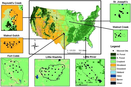
The U.S. Department of Agriculture’s (USDA) Agricultural Research Service (ARS) has installed seven in situ networks containing impedance-based soil moisture probes (Stevens Water hydraprobes) at a 5 cm depth for soil moisture estimation, as shown in Figure 1. These networks are distributed across a variety of scales of a moderate resolution for satellite remote sensing purposes (∼25–35 km). These networks are located in the Little River basin in Georgia (LR), the Little Washita River basin in Oklahoma (LW), Fort Cobb in Oklahoma (FC), the Reynolds Creek basin in Idaho (RC), the South Fork of the Iowa River (SF), the Walnut Gulch basin in Arizona (AZ), and the St. Joseph’s basin in Indiana (SJ). Some of these installations have been providing hourly soil moisture data since 2001 in the earliest cases and have formed the basis of numerous research objectives comparing in situ estimates to satellite estimates (Jackson et al. 2010; Jackson et al. 2012; Bindlish et al. 2015; Chan et al. 2016) and upscaling soil moisture measurements (Coopersmith et al. 2016; Clewley et al. 2017).

3. Methodology

Prior to beginning more detailed analysis on an individual watershed’s in situ network, we utilized the full length of the watershed’s record and obtained an ordinal ranking of the average soil moisture values reported at each individual sensor. We defined these values as $r_{i,\mathrm{all}}$, the rank of sensor i over all years. Additionally, the average and standard deviation of those values reported as the weighted network average soil moisture were recorded as ${\mu }_{\mathrm{WASM}}$ and ${\sigma }_{\mathrm{WASM}}$. The weighted network average was chosen by assigning weights to individual sensors within a network that roughly correspond to the proportion of the watershed for which their estimates are representative. For most of these watersheds, the soil moisture distribution was primarily influenced by precipitation patterns, which are assumed to be isotropic at this scale. These simple descriptive statistics provided a basis of comparison for the performances of individual sensors over the temporal intervals selected for further analysis.

3.1 Analysis by year

Within a given year y, we began by calculating $r_{i,y}$ for all sensors i. Next, these rankings are correlated with the values of $r_{i,\mathrm{all}}$ using the subset of rankings for which the sensor in question was active during year y, defined as the Spearman’s ρ coefficient (correlation of rank). Next, we visualized the values of $r_{i,y}$ over all values of y for each sensor, i, to ascertain qualitatively whether a sensor is consistently wetter or drier than the historical average in any given year.

Figure 1. The location of the seven ARS watersheds over a generalized landcover data layer.

3.2 Analysis by season

Next, analysis was performed using exclusively the values at each sensor during a specific month (e.g. all estimates in the sensor’s record during the month of June). Thus, for each month, a value of $r_{i,m}$ was calculated – the ranking of sensor i during month m. Much like the inter-annual analysis, an analogous rank correlation analysis was performed, comparing the ordinal rankings of wetness/dryness during any individual month m to the values of $r_{i,\mathrm{all}}$. Next, the values of $r_{i,m}$ were visualized over all values of m to ascertain qualitatively whether a sensor’s relative mean difference of wetness or dryness was a function of the month of the year. To avoid issues of freezing and thawing, only the months between April and October (inclusive) were chosen as values of m.

3.3 Combinatoric removals

To ascertain what proportion of sensors are required to generate a suitable estimate of the network average, subsets of the overall network were chosen and subsequently compared to the network average. The analysis begins with subsets of size 1, then subsets of size 2, and so on until subsets reached size n – 1, where n is the number of sensors within a given test watershed. In cases where there does not exist a sufficient number of timestamps where n – 1 sensors were active simultaneously, this analysis was halted at lower group sizes. It is important to note that the number of unique combinations of size k that were chosen from a set of size n is given by: (1) $({}_k^n)={\displaystyle \frac{n!}{k!(n-k)!}}$(1)

In Little River, the number of sensors within the network (n) was 33. The number of unique combinations of size 16 is in excess of one billion. This was computationally intractable. As a consequence, for cases where the value obtained by Equation (1) exceeds a pre-selected maximum (set to 1000 for the purposes of this analysis), a random selection of the maximum number of combinations was evaluated. Thus, for each value of k, below n, we calculated the following: (2) $\mathrm{RMS}{\mathrm{E}}_k={\sum }_i^{\min \left(1000,{\displaystyle \frac{n!}{k!(n-k)!}}\right)}{\displaystyle \frac{{\sum }_{t=1}^n\sqrt{{\displaystyle \frac{{({\mu }_{\mathrm{network},t}-{\mu }_{k,t})}^2}{n}}}}{\min \left(1000,{\displaystyle \frac{n!}{k!(n-k)!}}\right)}}$(2)

In Equation (2), $\mathrm{RMS}{\mathrm{E}}_k$ represents the average root-mean-squared-error associated with use of only k sensors within an n-sensor network. The mean of the complete network and the average calculated with the available subset of k sensors, at each time t, are signified by ${\mu }_{\mathrm{network},t}$ and ${\mu }_{k,t}$ respectively. Equation (3), analogous in several respects to Equation (2), calculates the standard deviation of the RMSE-values calculated for the k-sensor combinations, ${\sigma }_k$. This is a measurement of just how sensitive the $\mathrm{RMS}{\mathrm{E}}_k$ value from Equation (2) is to the specific combination of k sensors to which we have access. (3) ${\sigma }_k={\sum }_i^{\min \left(1000,{\displaystyle \frac{n!}{k!(n-k)!}}\right)}\sqrt{{\displaystyle \frac{{(\mathrm{RMS}{\mathrm{E}}_i-\mathrm{RMS}{\mathrm{E}}_k)}^2}{\min \left(1000,{\displaystyle \frac{n!}{k!(n-k)!}}\right)}}}$(3)

The only additional new term in Equation (3) is that of $\mathrm{RMS}{\mathrm{E}}_i$, the root-mean-square error for a specific combination i of k sensors.

Previous research evaluating three co-located profiles at U. S. Climate Reference Networks (CRN) revealed that the average measurement error associated with the Stevens Water Hydra probe measurements in the United States was approximately 0.012 m³/m³ (Coopersmith et al. 2015). As k is increased, $\mathrm{RMS}{\mathrm{E}}_k$ was subsequently compared to the inherent measurement error and/or, for watersheds where this level of uncertainty was not obtained, how many sensors are needed within the network to achieve $\mathrm{RMS}{\mathrm{E}}_k$ values lower than 110% of the above inherent measurement error or 1.1*$\mathrm{RMS}{\mathrm{E}}_{n-1}$ where n is the number of sensors within the network. In other words, how many sensors are required to remove ∼90% of the error that would be achieved with only one missing sensor.

4. Results

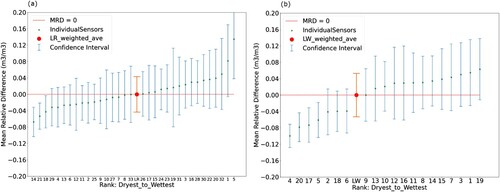
For each of the seven watersheds, we began with an image of the network’s sensors, ranked from driest to wettest from left-to-right, as shown in Figure 2. At each sensor, the green dot depicts the mean relative difference as compared with the overall network mean (the larger red dot). Furthermore, at each sensor, the standard deviation of soil moisture values reported by that sensor over its lifetime is represented by the blue error bars. The standard deviation of network average estimates is illustrated by the thicker green error bars about the larger red dot. In Figure 2(a), in Little River, sensors #1 and #5 are considerably wetter than the remaining sensors within the watershed, while sensors, #14, #18, and #21 are atypically dry. In these cases, even one full standard deviation below or above the sensor’s mean soil moisture value still only marginally brings the reported value within the vicinity of the network mean. In Figure 2(b), in Little Washita, it is noteworthy that rather than a smoothly, monotonically increasing set of sensors, seven sensors are decidedly wetter than the remaining thirteen. In this case, the results are likely the byproduct of a watershed containing two distinct soil textures, (sand and clay) leading to decidedly drier and wetter measurements, respectively.

Figure 2. Temporal stability plots of (a) Little River, Georgia and (b) Little Washita, Oklahoma. Error bars denote standard deviations of individual sensors’ reported values. Watershed weighted averages represent the overall watershed average, as determined by sensor positions and its’ associated confidence interval.

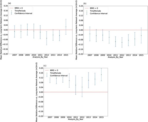
4.1 Analysis by year

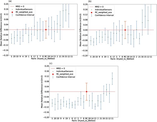
With overall distributions established, we plotted charts analogous to those presented in Figure 2, maintaining the same sequence of sensors from left-to-right, but presenting the distribution of values from within the given year. Three years are presented in this manner in Figure 3. While the ordering of sensors from driest to wettest is not identical to the ordering of the overall distribution, the same general pattern remains. Note that, in certain cases, a given sensor did not function during a given year, visualized as a single green dot with a mean relative difference of 0 and a null error bar.

Figure 3. Annual distributions in Reynolds Creek, Idaho. (a) 2004, (b) 2005, and (c) 2006. Error bars denote annual standard deviation of reported sensor values.

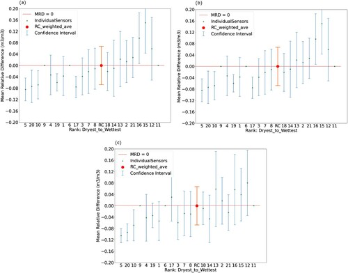
In Table 1, the correlation between the rankings of the active sensors and those sensors’ rank in the network’s overall distribution was calculated for every year in which a watershed’s network is in service. The number of active sensors is noted parenthetically. In total, sixty-seven such years were examined across the seven watersheds. Of these, only ten present a Spearman’s rho value below 0.8. Seven of these ten instances occur in the Reynolds Creek watershed. In most of the watersheds examined, these correlations remain fairly consistently above 0.85 and often exceed 0.9. A temporary network left in place for a full growing season is likely to suffice in gleaning the relative relationships between sensors.

Table 1. Annual rank correlations for each of the ARS watersheds.

Year	FC	LR	LW	RC	SF	SJ	WG
2001	–	.826 (8)	–	.641 (11)	–	–	–
2002	–	.859 (12)	–	.837 (16)	–	–	.883 (51)
2003	–	.785 (14)	–	.828 (16)	–	–	.895 (51)
2004	–	.731 (28)	–	.921 (18)	–	–	.871 (51)
2005	–	.860 (29)	–	.889 (18)	–	–	.896 (51)
2006	–	.855 (31)	–	.840 (18)	–	–	.854 (51)
2007	.932 (15)	.854 (31)	.817 (20)	.723 (21)	–	.936 (7)	.834 (51)
2008	.943 (15)	.866 (31)	.805 (20)	.750 (19)	–	.958 (7)	.891 (51)
2009	.975 (15)	.924 (32)	.842 (20)	.754 (20)	–	.896 (7)	.890 (51)
2010	.975 (15)	.908 (32)	.903 (17)	.853 (20)	–	.949 (11)	.907 (51)
2011	.893 (15)	.854 (32)	.845 (20)	.795 (20)	–	.931 (11)	.932 (51)
2012	.882 (15)	.852 (30)	.893 (20)	.737 (19)	–	.731 (13)	.900 (51)
2013	.861 (15)	.927 (28)	.908 (20)	.894 (18)	.904 (20)	.957 (13)	.947 (51)
2014	.875 (15)	.951 (28)	.860 (18)	.772 (19)	.872 (20)	.939 (12)	.906 (51)

In addition to analysis by year in terms of rank, individual sensors’ distributions within watersheds were examined on a year-by-year basis to ascertain whether or not their behavior is annually consistent. Figure 4 presents three individual sensors within the Fort Cobb basin (OK).

Figure 4. Fort Cobb, Oklahoma, sensor distributions by year. (a) Sensor #6, (b) Sensor #7, (c) Sensor #13. Error bars denote annual standard deviation of reported sensor values.

In Figure 4, we can distinguish three types of sensors. All three note a slightly drier year in 2011 and 2012. Figure 4(a), l depicts a sensor that is consistently dry, throughout the decade for which it is installed. Figure 5(b) shows is a sensor that is consistently around the overall network mean. Figure 5(c) shows a sensor that is consistently wetter than the network as a whole. This corroborates the findings of Table 1, that these relative relationships (which sensors are wetter/drier) are typically stable temporally.

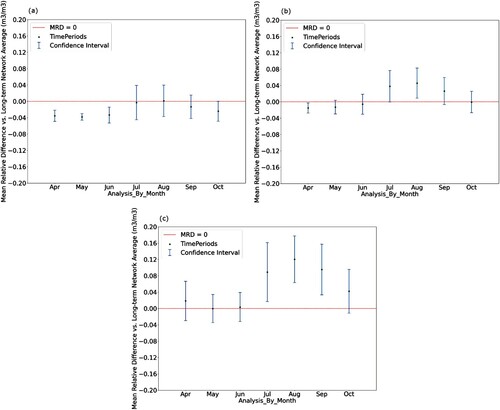
Figure 5. Temporal stability plots for Reynolds Creek, Idaho. (a) May, (b) June, (c) July. Error bars denote monthly standard deviation of reported sensor values.

4.2 Analysis by month

Figure 5 presents a triad of images from the Reynolds Creek basin in Idaho, illustrating the distribution of each sensor using only data from the months of May, June, and July, respectively. With the spring months receiving considerably greater quantities of precipitation each year, we note that soil moisture values are typically higher during May than in July. While by mid-summer, the majority of sensors report values that are well below the historical network average, the overall trend remains – that is, those sensors that are drier/wetter in one month tend to be the same sensors that are drier/wetter in another. It is worth noting that these relationships are more robust in watersheds where rain is received regularly in every month. By contrast, in certain watersheds, meaningful rainfall is only received during one or two months of the year. In the months where rainfall is not received, there is little that distinguishes the soil moisture content at one sensor from that at another – all sensors quickly return to their minimum possible values (residual soil moisture) and remain there until months when sufficient precipitation arrives.

Table 2 presents findings that are similar to those presented in Table 1, with the analytical subsets being determined by the month of the year rather than the year within the watershed network’s history. Like Table 1, the number of available sensors is noted parenthetically, to the right of the calculated Spearman Rho correlation.

Table 2. Monthly rank correlation for each ‘warm’ month for each watershed.

Year	FC	LR	LW	RC	SF	SJ	WG
Apr.	.953 (15)	.945 (33)	.895 (20)	.961 (21)	.892 (20)	.925 (15)	.798 (50)
May	.989 (15)	.973 (33)	.964 (20)	.907 (21)	.847 (20)	.982 (15)	.811 (51)
June	.954 (15)	.952 (33)	.967 (20)	.675 (21)	.811 (20)	.929 (15)	.854 (50)
July	.961 (15)	.948 (33)	.886 (20)	.675 (21)	.863 (20)	.939 (15)	.860 (51)
Aug.	.950 (15)	.960 (33)	.937 (20)	.657 (21)	.704 (20)	.914 (15)	.870 (51)
Sep.	.957 (15)	.961 (33)	.830 (20)	.767 (21)	.802 (20)	.961 (15)	.889 (51)
Oct.	.993 (15)	.968 (33)	.928 (20)	.916 (21)	.710 (20)	.961 (15)	.914 (51)

These correlations were even stronger than their annual analogs. Of forty-nine months examined, only seven display a correlation below 0.8. Four of these seven are during the dry summer in Reynolds Creek (Idaho) and another falls in the dry spring in Walnut Gulch (Arizona). Of the remaining forty-two months, twenty-nine of them showed a correlation above 0.9. As mentioned previously, during months when little, if any rain occurs, it was more difficult for the rankings among sensors to be retained, as most/all measurements fell to residual soil moisture values.

Figure 6 presents a triad of images from the Walnut Gulch. In southern Arizona, rainfall was generally limited to the monsoon season, during late July, August, and September. As a result, all images displayed the same seasonal pattern. However, in Figure 6(a), sensor #18, was consistently drier than the network average, in Figure 6(b), sensor #36, is near the network average, while sensor #2, in Figure 6(c), is decidedly wetter than the network average throughout the year. Also notable is the fact that the remaining four months, where limited rain occurs, assume roughly the same value. Nonetheless, these findings confirmed what is presented in Table 2 – seasonal relationships are stable in both wetter and drier sensors – relative wetness was not a function of the season in which the analysis occurs.

Figure 6. Walnut Gulch, Arizona, sensor distributions by month. (a) Sensor #18, (b) Sensor #36, (c) Sensor #2. Error bars denote monthly standard deviation of reported sensor values.

4.3 Combinatorics – the stability of incomplete networks

With an understanding from the previous two analyzes that relative intra-sensor relationships are stable both seasonally and year-to-year, the follow-up question is how many sensors are required to approximate the network average. In Figure 7, the network in South Fork, Iowa was examined by considering all combinations of one sensor, all combinations of two sensors, and so on, until the full network, less a single sensor is considered. For simplicity, when more than 1000 combinations are possible, only one random set of 1000 combinations is considered. See Equations (2) and (3) for additional detail.

Figure 7. Triple colocation error for an increasing number of sensors at the South Fork, network.

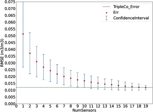
In Figure 7, though it is clear that each additional sensor decreases the error associated with the partial network, there are diminishing marginal returns. A combination of 16 of the 20 available sensors will produce an average error against the overall network mean that is within 110% of the inherent uncertainty associated with Hydraprobe measurements. Table 3 presents these values for the remaining watersheds.

Table 3. Number of sensors needed to estimate full network average for each watershed. Walnut Gulch is not included in this analysis as no timestamp contain all 54 sensors was available.

Watershed	# Sensors (To attain 110% of 0.012 m^3/m^3 or 110% of the RMSE for n − 1 sensors)	# Total Sensors
Fort Cobb	7	15
Little River	13	33
Little Washita	12	20
Reynolds Creek	11	20
St. Joseph’s	11	13
South Fork	16	20

In Table 3, though the seven watersheds contain highly disparate numbers of total sensors (from 13 in St. Joseph’s to 33 in Little River), the number of sensors beyond which the marginal utility of each additional instrument becomes small is more stable. No network requires more than 16 sensors (South Fork), and the remaining networks allow sufficient estimates with 13 or fewer sensors.

5. Discussion & conclusions

With instrumentation purchase, installation, and maintenance of permanent networks requiring considerable and sustained investment, this analysis helped to determine the viability of and quantitative requirements for a temporary network for scaling of a permanent network. From Table 3, it is found that approximately 12 sensors are sufficient in most environments, presuming their locations are distributed such that they capture the hydrologic heterogeneity of the watershed as well as the average moisture condition. This confirms the findings of Martinez-Fernandez and Ceballos (2005), though for a much longer time frame and much more diverse set of hydroclimatic conditions. The findings in Tables 1 and 2 suggest that the intra-sensor relationships are stable inter-annually and inter-seasonally. Therefore, if 12 sensors (stations) are deployed temporarily for one calendar year, it may be possible to scale a singular permanent station so that it estimates the average soil moisture of the location with similar confidence to the temporary network. Enhancing these estimates with models could allow increasingly accurate watershed network approximations with fewer and fewer sensors.

As a result of this temporal stability analysis, it is now possible, when a given sensor’s estimate is unavailable for a brief period, for its value to be replaced (based on its expected mean relative difference) rather than presenting the watershed average as the weighted average of the remaining active sensors. If the network’s wettest sensor is unavailable for a day, the current methodology uses the average of the remaining sensors, which will necessarily lead to a drier watershed-scale estimate.

Finally, by comparing the results between multiple watersheds, we begin to understand the long-term stability of the behavior of the soil moisture readings at a given location. This type of analysis illustrates seasonal patterns of soil moisture and inter-annual trends, especially in those watersheds whose networks have been installed for 15–20 years. It was determined that sensors can have stable patterns of soil moisture from one year to the next, which was previously established in Cosh et al. (2006), but now is confirmed for each of the watersheds in question.

Acknowledgement

This research was a contribution from the Long-Term Agroecosystem Research (LTAR) network. LTAR is supported by the United States Department of Agriculture and available through the National Agricultural Library or STEWARDS database. USDA is an equal opportunity employer and provider.

Disclosure statement

No potential conflict of interest was reported by the author(s).

Notes

Notes: Numbers in parentheses refer to the number of sensors available for that year of study. All correlations are significant with a p-value of less than 0.01.

Note: Number of available sensors used in the study for each watershed in parentheses.

References

- Belair, S., G. Balsamo, J.-F. Mahfouf, and G. Deblonde. 2005. “Towards the Inclusion of Hydros Soil Moisture Measurements in Forecasting Systems of the Meteorological Service of Canada.” IGARSS 4: 2741–2743. Art. 1525624.
- Bell, J. E., E. Weng, and Y. Luo. 2010. “Ecohydrological Responses to Multifactor Global Change in a Tallgrass Prairie: A Modeling Analysis.” Journal of Geophysical Research 115: G04042. doi:https://doi.org/10.1029/2009JG001120
- Bindlish, Rajat, Thomas Jackson, M. H. Cosh, Tianjie Zhao, and Peggy O’Neill. 2015. “Global Soil Moisture from the Aquarius/SAC-D Satellite: Description and Initial Assessment.” IEEE Geoscience and Remote Sensing Letters 12 (5): 923–927.
- Campoy, A., A. Ducharne, F. Cheruy, F. Hourdin, J. Polcher, and J. C. Dupont. 2013. “Response of Land Surface Fluxes and Precipitation to Different Soil Bottom Hydrological Conditions in a General Circulation Model.” Journal of Geophysical Research 118 (19): 10725–10739.
- Chan, Steven K., R. Bindlish, P. E. O’Neill, E. Njoku, T. J. Jackson, A. Colliander, F. Chen, et al. 2016. “Assessment of the SMAP Passive Soil Moisture Product.” IEEE Transactions on Geoscience and Remote Sensing 54 (5): 4994–5007. doi:https://doi.org/10.1109/TGRS.2016.2561938.
- Clewley, Daniel, Jane B. Whitcomb, Ruzbeh Akbar, Agnelo R. Silva, Aaron Berg, Justin R. Adams, Todd Caldwell, Dara Entekhabi, and Mahta Moghaddam. 2017. “A Method for Upscaling In Situ Soil Moisture Measurements to Satellite Footprint Scale Using Random Forests.” IEEE Journal of Selected Topics in Applied Earth Observations and Remote Sensing 10 (6): 2663–2673. doi:https://doi.org/10.1109/JSTARS.2017.2690220.
- Coopersmith, E. J., M. H. Cosh, J. E. Bell, and W. T. Crow. 2016. "Multi-Profile Analysis of Soil Moisture Within the U.S. Climate Reference Network.” Vadose Zone Journal 1–8. doi:https://doi.org/10.2136/vzj2015.01.0016.
- Coopersmith, E. J., M. H. Cosh, W. Petersen, J. Prueger, and J. Niemeier. 2015. “Soil Moisture Model Calibration and Validation: An ARS Watershed on the South Fork Iowa River.” Journal of Hydromet 1087–1101. doi:https://doi.org/10.1175/JHM-D-14-0145.1.
- Coopersmith, E. J., B. S. Minsker, C. E. Wenzel, and B. J. Gilmore. 2014. “Machine Learning Assessments of Soil Drying for Agricultural Planning.” Computers and Electronics in Agriculture 104: 93–104. doi:https://doi.org/10.1016/j.compag.2014.04.004.
- Cosh, M. H., T. J. Jackson, P. Starks, and G. Heathman. 2006. “Temporal Stability of Surface Soil Moisture in the Little Washita River Watershed and its Applications in Satellite Soil Moisture Product Validation.” Journal of Hydrology 323 (1–4): 168–177. doi:https://doi.org/10.1016/j.jhydrol.2005.08.020.
- Cosh, M. H., P. J. Starks, J. A. Guzman, and D. N. Moriasi. 2014. “Upper Washita River Experimental Watersheds: Multiyear Stability of Soil Water Content Profiles.” Journal of Environmental Quality 43 (4): 1328–1333. doi:https://doi.org/10.2134/jeq2013.08.0318
- De Rosnay, P., M. Drusch, D. Vasiljevic, G. Balsamo, C. Albergel, and L. Isaksen. 2013. “A Simplified Extended Kalman Filter for the Global Operational Soil Moisture Analysis at ECMWF.” Quarterly Journal of the Royal Meteorological Society 139 (674): 1199–1213.
- Grayson, R. B., A. W. Western, F. H. S. Chiew, and G. Bloschl. 1997. “Preferred States in Spatial Soil Moisture Patterns: Local and Nonlocal Controls.” Water Resources Research 33 (12): 2897–2908. doi:https://doi.org/10.1029/97WR02174.
- Jackson, T. J., R. Bindlish, M. H. Cosh, T. Zhao, P. J. Starks, D. D. Bosch, M. S. Seyfried, et al. 2012. “Validation of Soil Moisture Ocean Salinity (SMOS) Soil Moisture Over Watershed Networks in the U.S.” IEEE Transactions of Geoscience and Remote Sensing 50 (5): 1530–1543.
- Jackson, T. J., M. H. Cosh, R. Bindlish, P. J. Starks, D. D. Bosch, M. S. Seyfried, D. C. Goodrich, M. S. Moran, and J. Du. 2010. “Validation of Advanced Microwave Scanning Radiometer Soil Moisture Products.” IEEE Transactions of Geoscience and Remote Sensing 48: 4256–4272.
- Joetzjer, E., H. Douville, C. Delire, and P. Ciais. 2013. “Present-Day and Future Amazonian Precipitation in Global Climate Models: CMIP5 Versus CMIP3.” Climate Dynamics 41 (11-12): 2921–2936.
- Jones, A. S., J. Cogan, G. Mason, and G. McWilliams. 2010. “Design of a Temporal Variational Data Assimilation Method Suitable for Deep Soil Moisture Retrievals Using Passive Microwave Radiometer Data.” 2010 11th Specialist Meeting on Microwave Radiometry and Remote Sensing of the Environment 60–62. doi:https://doi.org/10.1109/MICRORAD.2010.5559591.
- Koster, R. D., and P. C. D. Milly. 1997. “The Interplay Between Transpiration and Runoff Formulations in Land Surface Schemes Used with Atmospheric Models.” Journal of Climate 10 (7): 1578–1591.
- Martinez-Fernandez, J., and A. Ceballos. 2005. “Mean Soil Moisture Estimation Using Temporal Stability Analysis.” Journal of Hydrology 312: 28–38.
- Sheffield, J., G. Goteti, F. Wen, and E. F. Wood. 2004. “A Simulated Soil Moisture Based Drought Analysis for the United States.” Journal of Geophysical Research 109 (24): 1–19. doi:https://doi.org/10.1029/2004JD005182
- Starks, P. J., G. C. Heathman, T. J. Jackson, and M. H. Cosh. 2006. “Temporal Stability of Soil Moisture Profile.” Journal of Hydrology 324 (1–4): 400–411. doi:https://doi.org/10.1016/j.jhydrol.2005.09.024
- Vachaud, G., A. Passerat De Silans, P. Balabanis, and M. & Vauclin. 1985. “Temporal Stability of Spatially Measured Soil Water Probability Density Function.” Soil Science Sociey of America Journal 49: 822–828.