A virtual geographic environment for dynamic simulation and analysis of tailings dam failure

ABSTRACT

It is of great significance for disaster prevention and mitigation to carry out disaster simulations for dam failure accidents in advance, but at present, there are few professional systems for disaster simulations of tailings dams. In this paper, we focused on the construction of a virtual geographic environment (VGE) system that provides an effective tool for visualizing the dam-break process of a tailings pond. The dam-break numerical model of the tailings dam based on computational fluid dynamics (CFD) was integrated into the VGE system. The infrastructure of the VGE was supported by a 3-D geographic information system (GIS) with a user-friendly interface for the initiation, visualization, and analysis of the dynamic process of tailings dam failure. Key technologies, including the integration of numerical models, rendering of large-scale scenes, and optimizations of disaster simulation and visualization, were discussed in detail. In the prototype system, information on the run-out path, travel distance, etc. can be obtained to visually describe the flow motion released by two dam failure cases. The simulation results showed that the VGE can be used for the multidimensional, dynamic and interactive visualization of dam-break disasters, and can also be useful for assessing the risk associated with tailings dams.

KEYWORDS:

• Vitrual geographic environment
• tailings dam break
• computational fluid dynamics
• spatiotemporal process simulation
• visualization analysis

1. Introduction

A tailings dam is typically an earth-fill embankment dam that is used to store toxic and potentially radioactive tailings (a slurry of fine particles) discharged from ore separation. Globally, due to the large number and various natural and human-induced factors (Azam and Li 2010; Rico et al. 2008b), dam-break accidents of tailings reservoirs have occurred time after time, which has caused catastrophic environmental pollution and the loss of property and human life, such as the Mount Polley accident in 2014, Samarco’s Fundão tailings dam crash in 2015, and Brumadinho’s Feijão tailings dam disaster in 2019. It is a challenging task for the government and the mining industry to prevent or at least minimize the potential hazard that a tailings dam failure brings. Therefore, the study of simulating and predicting the likely destroyed area from such a failure is of considerable significance to the mining industry.

To predict the area that may be inundated by a tailings dam accident, historical dam-break cases of tailings ponds have been collected for statistics and analysis to obtain an empirical regression equation (Larrauri and Lall 2018; Rico, Benito, and Diez-Herrero 2008a). Through this equation, the volumes of tailings released and the destroyed area of a tailings dam failure can be estimated based on the dam height and impounded volume. However, the predicted results may deviate from realistic tailings dam failure based on empirical regression because only two factors, the dam height and reservoir capacity, are considered.

Computational fluid dynamics (CFD), based on the law of conservation of physics, uses computer technology to accurately simulate and analyze problems that involve fluid flow, and it has become a widely accepted methodology that has been applied in a variety of environmental fields, including air pollution (Amorim et al. 2013), hydrology (Biscarini, Di Francesco, and Manciola 2010), landslides (Pastor et al. 2009, 2014), etc. Currently, there have been studies on the application of CFD to the simulation and prediction of tailings dam failure, such as rheological tests of tailings flow (Gao and Fourie 2015; Henriquez and Simms 2009), simple deposition simulations of tailings fluid (Babaoglu and Simms 2017; Gao and Fourie 2019; Luo, Xu, and Zhao 2017), and simulations of tailings disasters in real terrain (Wang et al. 2018; Yu, Tang, and Chen 2020). Therefore, the numerical simulation method based on CFD is considered to be a better choice to predict or rebuild the process of tailings dam failure.

Tailing dam failure is a complex geographic phenomenon involving dynamic processes. The results of numerical simulation of tailings disasters provide reliable estimation of the future status for decision makers to consider potential consequences, but representing them in an adequate space–time is limited (Havenith, Cerfontaine, and Mreyen 2019). As the visualization facilitates understanding the simulated results, how the information represents could be designed and used became an important issue. A conceptual framework of visual variables (position, size, shape, texture, etc.) was proposed to allow us to graphically represent geospatial information (Bertin 1983). Later work extended visual variables to include dynamic variables such as frequency and duration (Carpendale 2003) and 3-D display variables such as perspective height, camera posture (Slocum et al. 2003). The concept of geovisualization emerged (Çöltekin et al. 2017) to refer to any visual display featuring geospatial information (maps, imagery, 3-D models, etc.), broadening understanding of map roles. Geovisual analytics develops on the basis of geovisualization and refers to the science of using interactive visual interfaces for analytical reasoning with spatial information (Andrienko et al. 2007). In contrast to geovisualization, geovisual analytics focuses on supporting analytical reasoning methods to find interesting patterns from massive spatial datasets. However, both geovisualization and geovisual analytics emphasize the representation and analysis of spatial data, lacking the organization of space–time data and geographic models, and thus not possessing the ability to completely simulate geographic phenomena.

For the same purpose of visualizing geospatial space, the concepts of digital earth and virtual geographic environments (VGEs) were put forward by Gore (1998) and Lin and Gong (2001) respectively. Both emphasize the utilization of information technology to digitally reproduce the real geographic environment. Among them, digital earth is dedicated to digitizing the entire space–time changes of the Earth's environment to form a virtual globe (Guo, Liu, and Zhu 2010). The realization of a complete digital earth is a long-term goal, and due to the constraints of current technology, most of the digital earth applications that have been developed so far are based on mass storage technology and use earth observation (EO) data to describe the Earth in 2-D or 2.5-D at multiple resolutions, scales, and times. The term VGE originated because one can also use visual environments to represent geographic environments and to simulate the dynamic processes that take place in them.

The term VGE is defined as a digital geographic environment generated by merging geographic information technology, virtual reality technology, multichannel human–computer interactions and geographic modeling and simulation that users can use for recognizing and experiencing complex geographic phenomena and further geographic analysis (Chen and Lin 2018; Chen et al. 2013b; Lin and Chen 2015). After several stages of evolution, the VGE has formed a consensus on a dual-core (geodata and geomodel), four-module (data module, modeling and simulation module, expression module, and collaboration module) framework (Lin, Zhu, and Chen 2018; Lü 2011), and it is considered to be a new generation of geographic analysis tools after geographic information systems (GISs) (Chen et al. 2015; Lin et al. 2013; Lü et al. 2018; Rink et al. 2018). Integrated geographic modeling and simulation is a means to improve the exploration of geographic evolution processes or the geographical environment (Chen et al. 2020; Yue et al. 2016).

By coupling geographic models or other multidisciplinary models (e.g. the calculation model of solar radiation), the VGE has advantages that do not exist in traditional GISs, such as multidimensional visualization, dynamic geographic process simulation or prediction (Lin, Zhu, and Chen 2018; Lü et al. 2018), which has recently gained increasing attention from geoscientists associated with disaster simulation (Avagyan et al. 2018; Liu et al. 2017; Rink et al. 2018; Xu et al. 2010, 2011; Yin et al. 2017; Li et al. 2013, 2020, 2021; Zhu et al. 2016;), geographical experiments (Hu et al. 2011), plant growth simulation (Tang et al. 2019a; Tang, Yin, and Chen 2019b), and human behavior simulations (Chen et al. 2013a; Huang et al. 2018; Shen et al. 2018). For example, Xu et al. (2011) integrated the Pennsylvania State University–National Center for Atmospheric Research (PSU/NCAR) mesoscale model into the VGE; this model can not only represent static virtual geographic objects, such as terrain, buildings, and ocean but also predict the trends of air pollution diffusion by embedding the simulation results. Zhu et al. (2016) constructed a virtual geographic environment for a dam break risk analysis of the Xiaojiaqiao barrier lake in Anxian County, Sichuan Province, China. Li et al. (2021) proposed a rapid 3-D reproduction system of dam-break floods constrained by post-disaster information. Although the potential advantages of VGEs in geohazard research are recognized, there are very few applications in this field (Havenith, Cerfontaine, and Mreyen 2019).

Simulation of tailings dam failure phenomena in a virtual geographic environment can contribute to decision making. For example, numerical dam-break experiments can be conducted instead of actual geographic experiments which may be expensive or practically infeasible. Modeling and simulation environments are core components that prepare VGEs for geographic analysis (Chen and Lin 2018). In this paper, we investigate a reliable simulation model for tailings dam failure based on CFD and integrate it as a model module to develop a professional VGE that can simulate complex geographical processes or serve as an early warning system for tailings dam failure in an intuitive, dynamic, and interactive manner.

2. Methods

2.1. Overall framework

According to the dual-core and four-module framework of the VGE (Lin, Zhu, and Chen 2018; Lü 2011), the overall architecture of the VGE oriented to dynamic simulation and analysis of tailings dam failure is described, as shown in Figure 1. The framework consists of four layers: a geodata layer, a geo-modeling layer, a geovisualization layer, and a user work layer. The bottom layer is the foundation of the VGE, which adopts the mixed storage of a file system and database and is a complex collection of heterogeneous geographic data sets that can be divided into remote and local sources. Remote sources are web-based services containing tile map services (TMS) and web map tile services (WMTS), whereas local sources include 3-D objects, digital elevation models (DEMs), satellite imagery, shape files, time-series field data of simulated results, and configuration data. These data with different sources, formats and scales are processed and transformed into a readable format at the data processing model to provide the basic virtual geographic environment data for the system.

Figure 1. Overall framework.

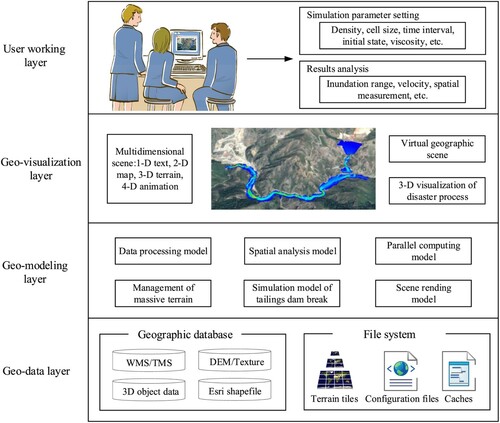
The geomodel layer is the core of the VGE and also includes terrain management, spatial analysis, tailings dam-break simulation and other models. In particular, the terrain management model is used to organize and deploy terrain data such as TMS, WMTS, DEMs, and satellite imagery that form a large-scale virtual scene (cf. Section 2.3). The spatial analysis model provides basic GIS functions such as spatial measurement, spatial annotation, visibility analysis, etc. Simulation module and parallel computing model are used for the numerical calculation and parallel optimization of tailings dam failure. The scene rendering module is used to ensure efficient rendering of large-scale terrain and simulated time series field data.

Based on the geomodel layer method, the geovisualization layer can provide the functions of geodata representation and the dynamic visualization of the disaster process. In addition, the geovisualization layer supports the multidimensional perception of virtual geographic scenes, such as 1-D text, 2-D map, 3-D virtual terrain, and 4-D animation of simulated field data, which can improve the spatial cognitive efficiency of dam-break disasters. At the top of the architecture is the user working layer directly oriented toward the end user involved in dam-break management. Users can set simulation parameters through the interactive interface and query and interactively analyze the simulation results in terms of velocity and inundation area to support their decision-making process.

2.2. Numerical model of the spatiotemporal process simulation

The simulation approach of tailings flow evolution after a dam-break based on CFD theory and the process of soundness verification were described in a previous study (Yu, Tang, and Chen 2020). In addition, for the failure of the Feijão tailings pond in Brazil on January 25, 2019, the error between the simulated tailings flow submerged area and the submerged area measured after the disaster is approximately 1.42%, indicating that the CFD approach can well simulate the dynamic process of tailings flow after dam failure on the 3-D terrain (Yu, Tang, and Chen 2020). In this paper, this simulation approach is used to simulate and predict the spatial process of tailings dam failure. In this approach, the continuity equation (Eq. 1) and the 3-D momentum equation (Eq. 2) are used as the motion control equations (Versteeg and Malalasekera 2007), and the rheological properties of the liquefied tailings fluid are described by the Bingham model (Eq. 3). (1) ${\displaystyle \frac{{\mathrm{\partial }}_{\rho }}{{\mathrm{\partial }}_t}+{\displaystyle \frac{{\mathrm{\partial }}_{\rho u_i}}{{\mathrm{\partial }}_{x_i}}=0}}$(1) (2) ${\displaystyle \frac{{\mathrm{\partial }}_{\rho u_i}}{\mathrm{\partial }t}+{\displaystyle \frac{{\mathrm{\partial }}_{\rho u_i{u}_j}}{\mathrm{\partial }{x}_j}=-{\displaystyle \frac{{\mathrm{\partial }}_p}{{\mathrm{\partial }}_{x_i}}+{\displaystyle \frac{\mathrm{\partial }}{\mathrm{\partial }{x}_j}\left[{\mu }_{eff}\left({\displaystyle \frac{{\mathrm{\partial }}_{u_i}}{\mathrm{\partial }{x}_j}+{\displaystyle \frac{{\mathrm{\partial }}_{u_j}}{\mathrm{\partial }{x}_i}}}\right)\right]+\rho g_i}}}}$(2) (3) ${\tau }_{ij}=\left({\displaystyle \frac{{\tau }_b}{\dot{\gamma }}+\mu }\right){\dot{\gamma }}_{ij}$(3) where $\rho$ is the density; $u_i$is the velocity; $t$ is the time; $p$ is the pressure; ${\mu }_{eff}$ is the effective viscosity; $g_i$ is the gravitational acceleration; ${\tau }_{ij}$ is the shear stress; ${\tau }_b$ is the yield stress; ${\dot{\gamma }}_{ij}$ is the rate-of-deformation tensor; and $\mu$ is the viscosity coefficient.

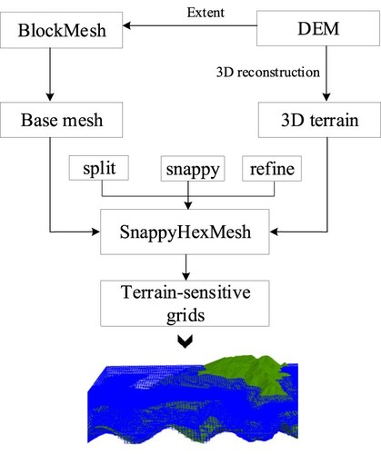
Furthermore, the most widely used numerical method in the field of fluid engineering, namely, the finite volume method (Versteeg and Malalasekera 2007), is used to solve the aforementioned governing equations numerically. The volume of fluid (VOF) method (Hirt and Nichols 1981) is used to track and locate the free surface of the tailings stream (the tailings stream-air interface) with the transport equation in Eq. 4. As shown in Figure 2, to consider the influence of terrain height fluctuations on the simulation results, the computational domain is divided into millions of hexahedral mesh cells based on a DEM. For more detailed descriptions or experiments, please refer to Yu (Yu, Tang, and Chen 2020). (4) ${\displaystyle \frac{\mathrm{\partial }ϝ}{\mathrm{\partial }t}+\mathrm{\nabla }\cdot (u_iϝ)=0}$(4) where function $ϝ$ is expressed as the volume fraction of tailings flow within the cell and takes values between 0 and 1.

Figure 2. Terrain-sensitive meshing process.

2.3. Rendering of large-scale scenes and field data

In this paper, the construction of the 3-D virtual scene mainly uses the open source scene graphics middleware OpenScenGraph (OSG), the 3-D terrain rendering engine osgEarth and the open graphics interface OpenGL. The virtual scene constructed is a virtual earth that can integrate terrain data of various resolutions around the world. Heterogeneous data such as raster, tile, vector, 3-D object and field data are the basis for this virtual globe. During development, these heterogeneous data increase the complexity and difficulty of data management and scene rendering in the system. In order to cope with these conditions, At the application level, to facilitate user management, the virtual scene data are organized in layers. Terrain, image, vector and entity 3-D model data are imported into the scene through the WMTS or SQLite database and are represented as the terrain layer, image layer, vector layer and model layer, respectively. With layers, users can switch between the layers they want to display, overlay a high-resolution layer on the low-resolution layer, set the transparency of different layers, remove and hide layers, etc.

At the development level, the technologies built in OSG and osgEarth (Wang and Qian 2010), such as directed acyclic graphs, quadtree indices, levels of detail, caching mechanisms, OpenGL state similarity sorting, scene culling, and paging databases, are used to organize data and optimize the rendering process, greatly improving the rendering efficiency. Additionally, multithreading technology is used to optimize rendering. The main thread is responsible for Cull and update operations, and the rendering objects after Cull are drawn in the sub-threads, taking advantage of the performance of multicore central processing units (CPUs) (Wang and Qian 2010). These technologies or methods made it possible to efficiently organize and render large-scale terrain scenes.

The numerical simulation results are organized as 3-D field data containing vector fields (e.g. velocity) and scalar fields (e.g. pressure and volume fraction). The field data characterize the distribution of physical quantities such as pressure and velocity in a certain space, i.e. each grid cell in the space is associated with several vector and scalar quantities. When rendering the field data, the vertex files and the mesh index files are first read, and the colorless 3-D mesh is reconstructed according to the discrete rules of the computational domain. After that, volume rendering or surface rendering is performed according to the distribution of scalars or vectors in the field data. Isosurfaces are the most common approach in surface rendering, which visualizes field data in a more quantitative way by connecting grid cells with the same given values to understand scalar spatial variations and distributions. For a 3-D scalar field $\mathrm{P}\in \mathbb{R}$, given a specified value q, a set $S(q)$ of isosurfaces with respect to $q$ is defined as (5) $S(q)=\{v\in \mathrm{V}\mid f(v)=q\}$(5) where the vertex set $\mathrm{V}$ is a subset of ${\mathbb{R}}^3$; and $f(.)$ represents a mapping from a vertex $v$ to a scalar $p$. A grid cell ${\sigma }_j$ consisting of $n$ vertices is considered an active cell if $mi{n}_i(p_{ji})\le q\le ma{x}_i(p_{ji})$. The intersection of the edges of the active cell with the isosurface is called the isosurface vertex and is obtained using linear interpolation along the edges of the active cell in this paper. The intersection coordinate values $v_i$ ($x_i$, $y_i$, $z_i$) of two vertices ($v_{j1}$ and $v_{j2}$) of the active edges and the specified value $q$ are calculated using Eq. (6) $\{\begin{array}{c}{x}_i=x_{j1}+(q-p_{j1})\ast (x_{j2}-x_{j1})/(p_{j2}-p_{j1})\\ y_i=y_{j1}+(q-p_{j1})\ast (y_{j2}-y_{j1})/(p_{j2}-p_{j1})\\ z_i=z_{j1}+(q-p_{j1})\ast (z_{j2}-z_{j1})/(p_{j2}-p_{j1})\end{array}$(6)

2.4. Model integration

OSG and osgEarth are 3-D graphics and terrain rendering engines that focus on 3-D world representation and efficient rendering, but they are not complete game or simulation engines due to the lack of corresponding physical models, collision detection, audio processing and so on (Wang and Qian 2010). Therefore, the 3-D VGE based on OSG and osgEarth can efficiently render large-scale virtual geographic scenes, which provides a rendering basis for dam-break simulations of tailings ponds, but the lack of dam-break physical models makes it impossible to directly simulate the dynamic process of tailings dam failure. To solve this problem, we integrated the aforementioned CFD simulation approach into the developed virtual geographic scene to form a complete VGE platform for the simulation and analysis of tailings dam failure. Tailing dam failure is a dynamic phenomenon with spatiotemporal characteristics. Static maps representation emphasizes the geometry of the run-out path and travel distance, and it can be difficult to depict temporal aspects of tailings flow, e.g. velocity. Animation is a desirable method for spatiotemporal tasks. The time-series nodes of tailings flow movement ware placed on the surface of a 3-D globe.

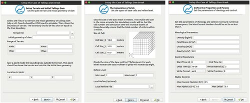
We employ the open field operation and manipulation (OpenFOAM), an open source library in the CFD field (Jasak, Jemcov, and Tukovic 2007), to implement the numerical calculation. OpenFOAM is a collection of hundreds of object-oriented functionality packages that can be flexibly called by commands and parameters in the VGE. A typical workflow (as shown in Figure 3) for simulating the spatial process of tailings dam failure in the VGE usually includes the following steps: (1) Set the relevant parameters of the spatial simulation, such as the DEM required for simulation in the model parameters dialog (as shown in Figure 4(a)), rheological parameters, case control parameters, and initial conditions. (2) Preprocess the computational grid and calibrate the simulation parameters to generate the configuration files needed for the simulation (as shown in Figure 4(b)). (3) Invoke the CFD calculation module according to the parameters in the configuration file (as shown in Figure 4(c)). The calculation time depends on the complexity of the grid, the simulation time range and the number of CPU cores, typically ranging from tens of minutes to dozens of hours. (4) The calculation results are parsed to generate the time-series nodes of tailings flow movement that are imported into the geographical scene, and these nodes can be geographically visualized and animated in the VGE through the playback control toolbar and panel.

Figure 3. Simulation workflow of dam-break disasters in the virtual geographic environment.

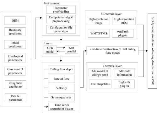
Figure 4. Parameters setting dialog.

2.5. Optimizations of disaster simulation and visualization

Generally, using a 3-D numerical model to solve the flow problem of tailings reservoir failure will face problems such as a large number of grids and extremely dense calculation tasks, resulting in the failure of serial computing to complete the simulation. Therefore, a CPU-based high-performance calculation (HPC) is used to allocate the intensive computing tasks to different CPU cores to reduce the time required for simulation.

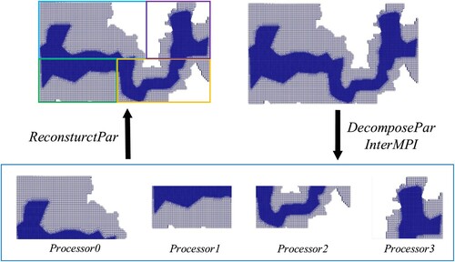
The parallel method we used is the region decomposition method, as shown in Figure 5. The DecomposePar tool built in OpenFOAM was used to slice the calculation grid into a specified number of subregions. After that, the relevant computing tasks of the subregions are distributed to different processing cores through InterMPI and a portable batch system (PBS). After the calculation task is completed, the ReconstructPar tool built in OpenFOAM is used to remerge the decomposed subregions into a complete grid for rendering.

Figure 5. Domain decomposition process.

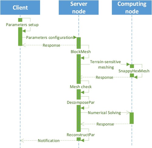
In addition, we design the VGE based on the client/server (C/S) architecture. When the client on personal desktop computer cannot meet the computing requirements, the computing resources of the server can be used to complete the simulation. The server can be deployed on a high-performance computer or cluster with multiple CPUs, in this case on a Fujian supercomputer. Figure 6 illustrates the parallel computing process in an HPC cluster, once the user has set up the relevant parameters, the client generates a parameter configuration file and transmits it to the server deployed in a cluster. Following receipt of the computation request and the simulation configuration, the server performs mesh generation, mesh verification and region decomposition, and then assigns the computation tasks of the decomposed regions to different computation nodes via InterMPI and PBS, as well as monitors the running status of the computation task. If the computational task is completed, the decomposed regions are merged and the client is notified of data completion.

Figure 6. UML sequence diagram of parallel numerical computing in a cluster.

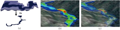
To render the 3-D field data of the dam-break disaster, we use the following methods to ensure rendering efficiency. (1) First, the value of all the physical quantities (e.g. velocity, pressure, etc.) of that time node is read in real time when each time node is rendered, and the colorless mesh is pseudocolor-mapped by the physical quantity specified. (2) In addition to the grid cells with tailings fluid, the colorless mesh also contains a large number of grid cells without tailings fluid. As shown in Figure 7(a), we use the alpha quantity (i.e. volume fraction of fluid) to cut out the grid cells without tailings fluid in the mesh before rendering to smoothly render the simulated animation of the dam-break disaster. (3) To play the animation without stutter, double-buffer technology is used in the rendering process of simulation results. When rendering the simulation results of the current time node, the next time node is preloaded and processed in memory so that it can be directly delivered to the GPU, which saves processing time. (4) Furthermore, the simulation results can be rendered in the form of surfaces, points and wireframes (as shown in Figure 7(b,c)) to further reduce the complexity of the rendering object.

Figure 7. Mesh clipping and different rendering forms of simulation results: (a) diagram of mesh clipping; (b) simulation result rendered in surface form; and (c) simulation result rendered in wireframe form.

3. Application prototype

3.1. System implementation

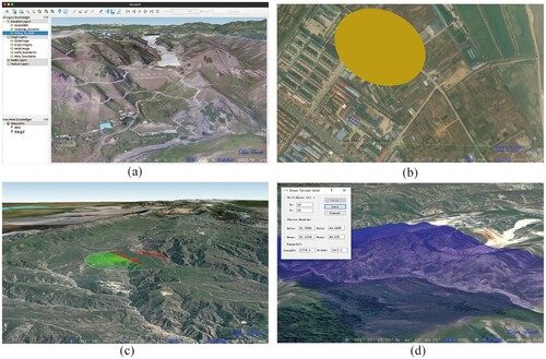
According to the above methods, the VGE prototype system for dam-break simulation of a tailings pond was implemented in C++ using Qt Creator 4.5. The system includes a client and a process server. The code heavily leverages open source libraries, including OSG and osgEarth for 3-D geographic scene rendering; OpenFOAM for numerical calculation of the model; QT for the design of the graphical user interface (GUI). The main interface of the developed TDBSim system is shown in Figure 8(a), which includes the following capabilities: web map/terrain data, such as Ready Map, Bing Map, and OpenStreetMap, are used as the basic layer of the global terrain scene, and a local high-resolution image/DEM, an ESRI shapefile, and a 3-D entity model (e.g. obj and stl) can be overlaid on it; The basic spatial analysis of the 3-D GIS, e.g. annotation, spatial measurement, and visibility analysis, is provided, as shown in Figure 8(b–d). Simulation and visual analysis of the dam-break disaster of a tailings pond can be carried out.

Figure 8. The main interface and some features of the prototype VGE: (a) main interface; (b) spatial annotation and measurement; (c) visibility analysis; and (d) terrain grid generation.

3.2. System applications

To demonstrate the applicability and effectiveness of the system, the Brumadinho tailings dam failure scenario and the A’xi tailings dam failure scenario were simulated in this section. The former is the event of a tailings pond collapse in Brazil on January 25, 2019, and the latter is the largest tailings pond still in operation in China's Xinjiang Uygur Autonomous Region.

3.2.1. Case 1: Brumadinho dam disaster

The Córrego do Feijão iron ore mine complex is located in the upper valley of the Paraopeba River in Brumadinho, and consists of two tailings dams (Tailings Dam I and Tailings Dam VI), an administrative office, and a small rail network for transporting iron ore. The Tailings Dam I was approximately 720 $\mathrm{m}$ long and 86 $\mathrm{m}$ high and stored approximately 12.7 million ${\mathrm{m}}^3$ of tailings (Porsani, Jesus, and Stangari 2019). On January 25, 2019, the sudden structural instability of Tailings Dam I resulted in a catastrophic failure that claimed 259 lives. According to postdisaster satellite remote sensing images and site investigations, the liquefied tailings flow of approximately 11.7 million ${\mathrm{m}}^3$ with high potential energy flowed more than 9 $\mathrm{km}$ to the lower elevation area, inundating a downstream area of more than 2.54 million ${\mathrm{m}}^2$ (including a small village) and eventually flowing into the Paraopeba River, which is the main river in the area (Porsani, Jesus, and Stangari 2019; Yu, Tang, and Chen 2020).

In the parameter settings dialog (Figure 4), a procedure is followed to set the simulation options. The 3-D terrain files required for the simulation are generated by the terrain grid-making function (Figure 7(d)) based on the ALOS PALSAR RTC DEM with a $12.5\mathrm{m}\times 12.5\mathrm{m}$ resolution. The computational mesh division takes into account the terrain, and the space size of the cell is set to 10 $\mathrm{m}$ × 10 $\mathrm{m}$ × 3 $\mathrm{m}$, generating 3,241,998 cells in total. Some specific settings are as follows: the dam body is assumed to instantaneously collapse completely, the simulated time range is 0$\mathrm{s}$–2500$\mathrm{s}$, the storage interval of the simulation results is 5 $\mathrm{s}$, the maximum Courant–Friedrichs-Lewy number is limited to no more than 0.5, and the initial tailings volume is 11.7 million ${\mathrm{m}}^3$ based on reports. (Porsani, Jesus, and Stangari 2019), and the values of viscosity and yield stress were set to 0.741 $\mathrm{Pa}\mathrm{s}$ and 59.82 $\mathrm{Pa}$ with reference to the literature related to tailings rheology testing (Gao and Fourie 2015; Henriquez and Simms 2009).

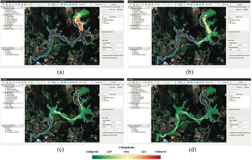
Figure 9 shows the comparison of the simulated and measured inundation areas from the Brumadinho accident, where the base map is the postdisaster remote sensing imagery of the Sentinel 2 satellite and the light cyan line is the actual measured boundary of the tailings flow. The numerically simulated tailings flow movement paths and inundation areas are in better agreement with the measured ones, with only minor differences at some locations. However, there is a noticeable difference in the location of the rail network, which is mainly because the simulation using DEM was collected in 2011, while the transportation railroad network was not yet completed in 2011. The simulated inundation area is approximately 2.572 $\mathrm{k}{\mathrm{m}}^2$, which is only 0.036 $\mathrm{k}{\mathrm{m}}^2$ different from the actual measured 2.536 km². In addition, more accurate DEM data and smaller cell sizes help to obtain better simulation results. However, a tailings dam break accident is a very complex geographic phenomenon, and the simulation results may not exactly match the actual results in time due to the existence of some factors that are not yet fully recognized, such as the solid–liquid separation phenomenon during motion.

Figure 9. Typical simulated results are visualized in TDBSim. The result is rendered at (a) $t=100\mathrm{s}$; (b) $t=300\mathrm{s}$; (c) $t=1000\mathrm{s}$; and (d) $t=2400.$ A – location of rail network. B – location of small community. C – location of Parque da Cachoeira. D – location of Paraopeba river. The base map is the satellite image (Sentinel S2). The color map of the simulation results is mapped by velocity characteristics.

3.2.2. Case 2: A’xi tailings dam

The second focus case within TDBSim is the A’xi Gold Mine dam, the largest tailings storage facility in the Xinjiang Uygur Autonomous Region of China, located in the Borokonu Mountains with large relief downstream. The A’xi tailings storage facility is a valley-type dam with a design capacity of approximately 3.6 million ${\mathrm{m}}^3$, dam length of 210 $\mathrm{m}$, width of 21 $\mathrm{m}$ and height of 58 $\mathrm{m}$. The multiyear average precipitation in the area where the gold mine is located is 428.1 $\mathrm{mm}$, and the maximum precipitation is 738 $\mathrm{mm}$, mainly from June to August (Huang 2016). There are several heavy rains in this area located in an earthquake-prone zone with an earthquake intensity of Ⅶ during the year, which may affect the production safety of the A’xi tailings dam (Wang 2014). Additionally, the A’xi Gold Mine tailings pond is located near the A’xi River Basin, a tributary of the Ili River, which is the main river for drinking water and agricultural irrigation downstream of Yining city. Consequently, once an accident occurs in the A’xi tailings dam, it will have an imperative impact on the downstream ecological environment and residents.

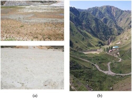
We conducted two field surveys of the A’xi Gold Mine in August 2018 and August 2019 using unmanned aerial vehicle (UAV) images of the area near the tailings impoundment to obtain a high-resolution DEM and digital orthomorphic model (DOM) and added them to the VGE to form a fine 3-D topography of the vicinity of the dam and downstream areas (Figure 10(a)). The dam is currently operating and stable, with two sets of millimeter-level monitoring equipment of dam deformation, two spill wells, and an environmental protection deposit (Figure 10(b)), and the height of the infiltration line is within safe limits. The tailings are press-filtered and discharged into the impoundment with a water content of approximately 22% and very small particles as dust tailings (Figure 10(a)), containing cyanide added during the beneficiation process. This dam is located in a sparsely populated alpine pastoral area, with no villages or people living within a few kilometers downstream, but the region is extremely ecologically fragile.

Figure 10. Field investigation photos of the A’xi tailings dam: (a) tailings in the A’xi tailings dam and (b) landforms downstream and environmental protection depot of the tailings dam.

Due to the limited shooting area acquired by the UAV, the ALOS PALSAR RTC DEM with a $12.5\mathrm{m}\times 12.5\mathrm{m}$ resolution is used for the downstream unphotographed area. The computational mesh division considers the terrain, and the space size of the mesh is set to 3 $\mathrm{m}$ × 3 $\mathrm{m}$ × 3 $\mathrm{m}$, generating 6,657,418 grid cells in total. Some specific settings are as follows: the dam body is assumed to instantaneously collapse completely, the simulated time range is 0$\mathrm{s}$–800$\mathrm{s}$, the storage interval of the simulation results is 5 $\mathrm{s}$, and the maximum Courant–Friedrichs-Lewy number is limited to no more than 0.5. Since the tailings storage facility is not currently experiencing a dam-break event, the initial tailings volume is estimated in this paper based on the empirical regression equation (Eq. 7) proposed by Larraur (Larrauri and Lall 2018) and is set at 75,6000 ${\mathrm{m}}^3$. (7) $\log (V_F)=-0.477+0.954\times \log (V_T)$(7) where $V_T$ is the current total storage capacity and $V_F$ is the estimated volume of tailings released after the dam collapse accident.

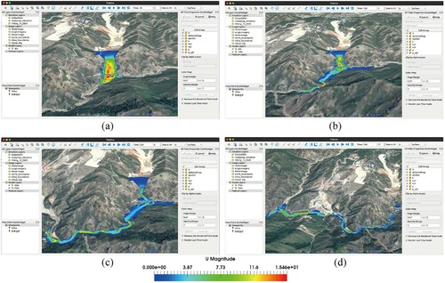
The same experiments and parameters were simulated in a previous study (Yu, Tang, and Chen 2020), and the simulation results are consistent with what was carried out in this paper in the TDBSim system, indicating that the CFD model is integrated into the VGE. Some of the typical simulation results are visualized in Figure 11. At 20 $\mathrm{s}$, the tailings flow released from the event first floods the environmental protection depot and switchyard approximately 250 $\mathrm{m}$ downstream of the tailings dam with a velocity of more than 15 $\mathrm{m}/\mathrm{s}$ and then enters the A’xi River valley approximately 320 $\mathrm{m}$ from the dam site and flows downstream along the valley topography. Although the valley elevation is greater than 155 $\mathrm{m}$ (within the calculated range), the valley is very tortuous, and the velocity of the tailings fluid gradually decreases. Finally, at 760 $\mathrm{s}$, the tailings flow reaches the simulated boundary with an average velocity of less than 2 $\mathrm{m}/\mathrm{s}$, at which point the flow distance is approximately 3.5 $\mathrm{km}$.

Figure 11. Typical simulated results are visualized in VGE. The result is rendered at (a) $t=30\mathrm{s}$; (b) $t=100\mathrm{s}$; (c) $t=250\mathrm{s}$; and (d) $t=760\mathrm{s}$.

From the numerical results, it can be seen that almost all of the tailings discharged after the failure of the tailings dam enter the A’xi River valley, except for some of the tailings that are blocked by the environmental protection depot. The normal runoff flow of the A’xi River is 0.5–2 ${\mathrm{m}}^3/\mathrm{s}$ and 0.002 ${\mathrm{m}}^3/\mathrm{s}$ during the dry season (Huang 2016), which is generally small, so the effect of water flow was not considered in the simulation. However, the region is prone to abnormal rainfall events, resulting in an increase in river runoff. Under such circumstances, the runoff flow of the A’xi River will increase, and the cyanide tailings will be continuously transported downstream by the river, which will seriously threaten the Guotou reservoir approximately 16 $\mathrm{km}$ downstream and the Ili River approximately 40 $\mathrm{km}$ downstream. Therefore, at the beginning of the accident, the inflow of contaminated water should be cut off immediately near the upstream part of the Guotou reservoir to avoid further damage.

3.3. System evaluation and discuss

The experimental environment is in the 64-bit Linux operating system. The CPU is a 3.6 GHz quad-core Intel Core I7-7700 CPU with 16 GB of RAM, and the graphics card is an NVIDIA GTX 1060 with 6 GB of RAM. The numerical computation server is installed in the Fujian supercomputing cluster with hundreds of CPU cores available for invocation. The performance of the TDBSim system is evaluated and discussed in terms of rendering efficiency, computational efficiency, and reasonableness of simulation.

For rendering efficiency, frame per second (FPS) is used as the benchmark to evaluate the rendering performance quantitatively. Figures 6–8 show the visual effects of the virtual globe and tailings fluid. The global data services provided by the spatial data infrastructure (SDI), including WMTS and WMS, as well as the local database of high-resolution UAV images can be viewed seamlessly in the system. Under the loading of approximately 50 GB of local imagery and DEM data, the rendering frame rate is between 300 FPS and 2000 FPS (as the amount and resolution of LOD-based in the viewpoint decreases gradually), resulting from the use of several rendering acceleration techniques in section 2.3, such as multithreaded rendering, LOD strategy, scene culling, etc. Rendering frame rates excess of 30 FPS after scalar-based clipping or generation isosurface on tailings flow field data generated by the simulation. It should be noted that the rendering cost of the virtual globe is not excluded in the experiment and the actual rendering FPS of the field data of tailings flow should be better. Thus, field tailings flow data can be interactively visualized and analyzed by users to support decision making in disaster response.

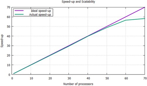
In terms of computation efficiency, for the large amount of computation in the 3-D numerical simulation process, based on the region decomposition method and CPU-based HPC technology mentioned in section 2.5, the decomposed computation tasks are assigned to different CPU cores on the server side through the InterMPI and PBS, effectively reducing the time required for the simulation computation process. Figure 12 shows the test results of the parallel method, and the maximum speed-up is close to 60 times on the supercomputer of Fujian Supercomputing Centre under more than 4 million grid cells. Nevertheless, the 3-D numerical simulation is still a time-consuming process. For the simulation of a Brumadinho disaster event whose computational domain was divided into 3,241,998 cells, the tailings flow was simulated using 40 CPU cores over a period of 2500 s, taking a total kernel time of approximately 13.12 h. For the dam-break simulation of the A’xi tailings dam whose computational domain was divided into 6,657,418 cells, the tailings flow was simulated using 40 CPU cores over a period of 800 s, taking a total kernel time of approximately 8.09 h.

Figure 12. Parallel scalability testing.

The reasonableness of the VGE simulation results for the run-out path and extent of tailings fluid from a tailings dam failure was verified by a historical tailings dam failure, where the accidental tailings flow path is consistent with that simulated by the system. The VGE is designed for interactive parameter configuration, simulation and visualization of tailings dam break disasters which is a very complex geographic phenomenon that makes it difficult to perfectly reproduce the accident process. Generally, the flow extent of tailings is affected by three factors: rheological model and parameters, the fineness of downstream topography, and boundary and initial conditions.

In the VGE, the rheological model used is the Bingham constitutive model which is commonly used to describe the rheological behavior of tailings fluids. The rheological parameters in this paper are taken from several studies (Gao and Fourie 2015; Henriquez and Simms 2009) related to tailings rheological testing. Users can perform rheological experiments for different cases to determine the appropriate rheological parameter settings. A fine downstream topography contains more detailed features and distinct terrain undulations than a coarse terrain model, making the numerical simulation results more consistent with the disaster phenomenon, but also increasing the computation time by a factor of several. Conversely, if the resolution of the terrain boundary is too low, detailed features of the terrain will be lost, which may result in large differences between the simulation results and the real events. The boundary condition is the variation law of each physical quantity on the boundary with time, and the initial condition is the spatial distribution condition of each physical quantity at the initial status. If the boundary conditions and initial conditions are not set reasonably, it may lead to the accumulation and propagation of errors, resulting in numerical dispersion or even collapse. The built-in boundary condition configuration scheme of the VGE is suitable for common tailings dam break simulation. The initial status of tailings flow is set at the location of the tailings pond according to the total volume released, which is more accurate than the traditional empirical equation to calculate the flow downstream curve because it is governed by laws of physics. The VGE supports the provision of interactive parameter setting dialogs and supports custom modification of the generated case configuration by professional users.

4. Conclusions and outlook

To reduce losses owing to tailings dam collapse incidents, the present work shows a generic framework for the development of a VGE for simulating and predicting the extent of damage caused by tailings dam failure. This framework has been demonstrated for the TDBSim system developed for disaster simulation of the Brumadinho dam disaster and the A’xi Gold Mine tailings dam. In particular, for the historical accident of the Brumadinho tailings dam, the simulated tailings flow path and inundation area closely matched the actual measured inundation area.

The presented VGE provides advantages in the third direction. First, the TDBSim integrates CFD-based numerical models that allow dynamic simulation of tailings dam failure in a more than reliable way than the empirical equations, which can be extended to the development of simulation systems for similar geographic phenomena such as reservoir dam failure and air pollution simulation. Second, methods such as volume rendering and isosurface are used to provide a smooth rendering effect for 3-D field data generated by numerical models. In addition, rendering acceleration techniques such as multithreaded rendering, LOD strategy, frustum culling, and occlusion culling are introduced to high-frame rendering of local spatial data and web data services provided by SDI. Third, based on template configuration, user-friendly interactive dialogs are provided to set simulation-related parameters and support professional users in making custom modifications to simulation config files. The simulated results can be interactively visualized and analyzed at a specific location and time, which are very important for decision-makers to make judgments.

Since the failure disaster of tailings dams is a complex geographic phenomenon involving rheology, hydrodynamics, geology and other multidisciplinary knowledge, it is unrealistic to perfectly reproduce the accident process. Future activities are related to considering solid–liquid separation during movement tailings flow and applying the framework to similar environmental studies within geohazard areas, for example, the diffusion of water/air pollution and mudslides. Furthermore, more than just parameter turning, we intend to provide a geo-collaboration environment of model sharing for experts during modeling. In addition, the emergence of technologies such as mixed reality, augmented reality and sensor networks greatly promote the development of virtual geographic environments, so we will introduce monitoring sensors in the VGE to provide safety warnings for tailings dams that are still in operation. Currently, the system is implemented on the desktop. With the trend of web-based modeling and simulation (Chen et al. 2020), this VGE can be transferred into a web-based environment.

Acknowledgments

We appreciate the three reviewers and editor(s) for their constructive comments that helped improve the quality of the paper. This research was funded by the National Key Research and Development Program of China (grant number 2017YFB0504203). The authors would like to thank Xiaoqin Wang Ph.D. from Fuzhou University for providing working facilities and financial support. The authors would like to thank the National Key Research and Development Project Team (2017YFB0504200) for the field investigative opportunity. The authors would like to thank Le Wang, Ph.D. from Xi’an Shiyou University for his expertise in CFD. The authors would like to thank the Supercomputing Center of Fujian for providing computing resources.

Disclosure statement

No potential conflict of interest was reported by the author(s).

Additional information

Funding

This work was supported by National Key Research and Development Program of China [grant number 2017YFB0504203].

References

- Amorim, J. H., V. Rodrigues, R. Tavares, J. Valente, and C. Borrego. 2013. “CFD Modelling of the Aerodynamic Effect of Trees on Urban air Pollution Dispersion.” Science of the Total Environment 461-462: 541–551.
- Andrienko, G., N. Andrienko, P. Jankowski, D. Keim, M. J. Kraak, A. MacEachren, and S. Wrobel. 2007. “Geovisual Analytics for Spatial Decision Support: Setting the Research Agenda.” International Journal of Geographical Information Science 21 (8): 839–857.
- Avagyan, A., H. Manandyan, A. Arakelyan, and A. Piloyan. 2018. “Toward a Disaster Risk Assessment and Mapping in the Virtual Geographic Environment of Armenia.” Natural Hazards 92 (1): 283–309.
- Azam, S., and Q. Li. 2010. “Tailings dam Failures: A Review of the Last One Hundred Years.” Geotechnical News 28 (4): 50–54.
- Babaoglu, Y., and P. H. Simms. 2017. “Simulating Deposition of High Density Tailings Using Smoothed Particle Hydrodynamics.” Korea-Australia Rheology Journal 29 (3): 229–237.
- Bertin, J. 1983. Semiology of Graphics: Diagrams, Networks, Maps. Madison: University of Wisconsin Press.
- Biscarini, C., S. Di Francesco, and P. Manciola. 2010. “CFD Modelling Approach for Dam Break Flow Studies.” Hydrology and Earth System Sciences 14 (4): 705–718.
- Carpendale, M. S. T. 2003. Considering Visual Variables as a Basis for Information Visualisation. Calgary: University of Calgary.
- Chen, M., and H. Lin. 2018. “Virtual Geographic Environments (VGEs): Originating from or Beyond Virtual Reality (VR)?” International Journal of Digital Earth 11 (4): 329–333.
- Chen, M., H. Lin, M. Hu, L. He, and C. Zhang. 2013a. “Real-Geographic-Scenario-Based Virtual Social Environments: Integrating Geography with Social Research.” Environment and Planning B: Planning and Design 40 (6): 1103–1121.
- Chen, M., H. Lin, O. Kolditz, and C. Chen. 2015. “Developing Dynamic Virtual Geographic Environments (VGEs) for Geographic Research.” Environmental Earth Sciences 74 (10): 6975–6980.
- Chen, M., H. Lin, Y. Wen, L. He, and M. Hu. 2013b. “Construction of a Virtual Lunar Environment Platform.” International Journal of Digital Earth 6 (5): 469–482.
- Chen, M., A. Voinov, D. P. Ames, A. J. Kettner, J. L. Goodall, A. J. Jakeman, M. C. Barton, et al. 2020. “Position Paper: Open web-Distributed Integrated Geographic Modelling and Simulation to Enable Broader Participation and Applications.” Earth-Science Reviews 207: 103223.
- Çöltekin, A., S. Bleisch, G. Andrienko, and J. Dykes. 2017. “Persistent Challenges in Geovisualization – a Community Perspective.” International Journal of Cartography 3 (Suppl. 1): 115–139.
- Gao, J. L., and A. Fourie. 2015. “Using the Flume Test for Yield Stress Measurement of Thickened Tailings.” Minerals Engineering 81: 116–127.
- Gao, J., and A. Fourie. 2019. “Studies on Thickened Tailings Deposition in Flume Tests Using the Computational Fluid Dynamics (CFD) Method.” Canadian Geotechnical Journal 56 (2): 249–262.
- Gore, A. 1998. “The Digital Earth: Understanding our planet in the 21st Century.” Presented at the Californian Science Center, Los Angeles, California, 31 January.
- Guo, H. D., Z. Liu, and L. Zhu. 2010. “Digital Earth: Decadal Experiences and Some Thoughts.” International Journal of Digital Earth 3 (1): 31–46.
- Havenith, H. B., P. Cerfontaine, and A. S. Mreyen. 2019. “How Virtual Reality Can Help Visualise and Assess Geohazards.” International Journal of Digital Earth 12 (2): 1–17.
- Henriquez, J., and P. Simms. 2009. “Dynamic Imaging and Modelling of Multilayer Deposition of Gold Paste Tailings.” Minerals Engineering 22 (2): 128–139.
- Hirt, C. W., and B. D. Nichols. 1981. “Volume of Fluid (VOF) Method for the Dynamics of Free Boundaries.” Journal of Computational Physics 39 (1): 201–225.
- Hu, M., H. Lin, B. Chen, M. Chen, W. Che, and F. Huang. 2011. “A Virtual Learning Environment of the Chinese University of Hong Kong.” International Journal of Digital Earth 4 (2): 171–182.
- Huang, Xihui. 2016. Analysis and Research on Feasibility Treatment Scheme of Dry Tailing Backfill in Open Pit. Wuhan: Wuhan Institute of Technology.
- Huang, L., J. Gong, W. Li, T. Xu, S. Shen, J. Liang, Q. Feng, D. Zhang, and J. Sun. 2018. “Social Force Model-Based Group Behavior Simulation in Virtual Geographic Environments.” ISPRS International Journal of Geo-Information 7 (2): 1–20.
- Jasak, H., A. Jemcov, and Z. Tukovic. 2007. OpenFOAM: A C++ Library for Complex Physics Simulations.
- Larrauri, P. C., and U. Lall. 2018. “Tailings Dams Failures: Updated Statistical Model for Discharge Volume and Runout.” Environments 5 (2): 1–10.
- Li, Y., J. Gong, J. Zhu, Y. Song, Y. Hu, and Y. Ye. 2013. “Spatiotemporal Simulation and Risk Analysis of Dam-Break Flooding Based on Cellular Automata.” International Journal of Geographical Information Science 27 (10): 2043–2059.
- Li, W., J. Zhu, L. Fu, Q. Zhu, Y. Guo, and Y. Gong. 2021. “A Rapid 3D Reproduction System of dam-Break Floods Constrained by Post-Disaster Information.” Environmental Modelling & Software 139: 104994.
- Li, W., J. Zhu, L. Fu, Q. Zhu, Y. Xie, and Y. Hu. 2020. “An Augmented Representation Method of Debris Flow Scenes to Improve Public Perception.” International Journal of Geographical Information Science 2020: 1–24.
- Lin, H., and M. Chen. 2015. “Managing and Sharing Geographic Knowledge in Virtual Geographic Environments (VGEs).” Annals of GIS 21 (4): 261–263.
- Lin, H., M. Chen, G. Lu, Q. Zhu, J. Gong, X. You, Y. Wen, B. Xu, and M. Hu. 2013. “Virtual Geographic Environments (VGEs): A New Generation of Geographic Analysis Tool.” Earth-Science Reviews 126: 74–84.
- Lin, H., and J. Gong. 2001. “Exploring Virtual Geographic Environments.” Geographic Information Sciences 7 (1): 1–7.
- Lin, H., Q. Zhu, and M. Chen. 2018. “The Being and Non-Being Generate Each Other, and the Virtual and the Real Are Mutually Interactive-The Progress of Virtual Geographic Environments (VGE) Studies in Last 20 Years.” Acta Geodaetica et Cartographica Sinica 47 (8): 1027–1030.
- Liu, M., J. Zhu, Q. Zhu, H. Qi, L. Yin, X. Zhang, B. Feng, H. He, W. Yang, and L. Chen. 2017. “Optimization of Simulation and Visualization Analysis of dam-Failure Flood Disaster for Diverse Computing Systems.” International Journal of Geographical Information Science 31 (9): 1891–1906.
- Lü, G. 2011. “Geographic Analysis-Oriented Virtual Geographic Environment: Framework, Structure and Functions.” Science China Earth Sciences 54 (5): 733–743.
- Lü, G., M. Chen, L. Yuan, L. Zhou, Y. Wen, M. Wu, B. Hu, Z. Yu, S. Yue, and Y. Sheng. 2018. “Geographic Scenario: A Possible Foundation for Further Development of Virtual Geographic Environments.” International Journal of Digital Earth 11 (4): 356–368.
- Luo, C., K. Xu, and Y. S. Zhao. 2017. “A TVD Discretization Method for Shallow Water Equations: Numerical Simulations of Tailing dam Break.” International Journal of Modeling Simulation and Scientific Computing 8 (3): 1–22.
- Pastor, M., T. Blanc, B. Haddad, S. Petrone, M. S. Morles, V. Drempetic, D. Issler, et al. 2014. “Application of a SPH Depth-Integrated Model to Landslide run-out Analysis.” Landslides 11 (5): 793–812.
- Pastor, M., B. Haddad, G. Sorbino, S. Cuomo, and V. Drempetic. 2009. “A Depth-Integrated, Coupled SPH Model for Flow-Like Landslides and Related Phenomena.” International Journal for Numerical and Analytical Methods in Geomechanics 33 (2): 143–172.
- Porsani, J. L., F.A.N.d. Jesus, and M. C. Stangari. 2019. “GPR Survey on an Iron Mining Area After the Collapse of the Tailings Dam I at the Córrego do Feijão Mine in Brumadinho-MG, Brazil.” Remote Sensing 11 (7): 1–13.
- Rico, M., G. Benito, and A. Diez-Herrero. 2008a. “Floods from Tailings Dam Failures.” Journal of Hazardous Materials 154 (1-3): 79–87.
- Rico, M., G. Benito, A. R. Salgueiro, A. Díez-Herrero, and H. G. Pereira. 2008b. “Reported Tailings Dam Failures: A Review of the European Incidents in the Worldwide Context.” Journal of Hazardous Materials 152 (2): 846–852.
- Rink, K., C. Chen, L. Bilke, Z. Liao, K. Rinke, M. Frassl, T. Yue, and O. Kolditz. 2018. “Virtual Geographic Environments for Water Pollution Control.” International Journal of Digital Earth 11 (4): 397–407.
- Shen, S., J. Gong, J. Liang, W. Li, D. Zhang, L. Huang, and G. Zhang. 2018. “A Heterogeneous Distributed Virtual Geographic Environment—Potential Application in Spatiotemporal Behavior Experiments.” ISPRS International Journal of Geo-Information 7 (2): 1–21.
- Slocum, T. A., D. C. Cliburn, J. J. Feddema, and J. R. Miller. 2003. “Evaluating the Usability of a Tool for Visualizing the Uncertainty of the Future Global Water Balance.” Cartography and Geographic Information Science 30 (4): 299–317.
- Tang, L., X. Peng, C. Chen, H. Huang, and D. Lin. 2019a. “Three-Dimensional Forest Growth Simulation in Virtual Geographic Environments.” Earth Science Informatics 12 (1): 31–41.
- Tang, L., D. Yin, and C. Chen. 2019b. “Optimal Design of Plant Canopy Based on Light Interception: A Case Study with Loquat.” Frontiers in Plant Science 10: 1–11.
- Versteeg, H. K., and W. Malalasekera. 2007. An Introduction to Computational Fluid Dynamics: The Finite Volume Method. Upper Saddle River: Pearson education.
- Wang, C. 2014. Study on Groundwater Pollution Evaluation and Prevention in A’xi Gold Mine. Xi'an: Chang'an University.
- Wang, R., and X. Qian. 2010. OpenSceneGraph 3.0: Beginner's Guide. Birmingham: Packt Publishing.
- Wang, K., P. Yang, K. Hudson-Edwards, W. S. Lv, C. Yang, and X. Jing. 2018. “Integration of DSM and SPH to Model Tailings Dam Failure Run-Out Slurry Routing Across 3D Real Terrain.” Water 10: 1087.
- Xu, B., H. Lin, L. Chiu, Y. Hu, J. Zhu, M. Hu, and W. Cui. 2011. “Collaborative Virtual Geographic Environments: A Case Study of air Pollution Simulation.” Information Sciences 181 (11): 2231–2246.
- Xu, B., H. Lin, L. S. Chiu, S. Tang, J. Cheung, Y. Hu, and L. Zeng. 2010. “VGE-CUGrid: An Integrated Platform for Efficient Configuration, Computation, and Visualization of MM5.” Environmental Modelling & Software 25 (12): 1894–1896.
- Yin, L., J. Zhu, Y. Li, C. Zeng, Q. Zhu, H. Qi, M. Liu, W. Li, Z. Cao, and W. Yang. 2017. “A Virtual Geographic Environment for Debris Flow Risk Analysis in Residential Areas.” ISPRS International Journal of Geo-Information 6 (11): 1–15.
- Yu, D., L. Tang, and C. Chen. 2020. “Three-Dimensional Numerical Simulation of Mud Flow from a Tailing Dam Failure Across Complex Terrain.” Natural Hazards and Earth System Sciences 20 (3): 727–741.
- Yue, S., M. Chen, Y. Wen, and G. Lu. 2016. “Service-Oriented Model-Encapsulation Strategy for Sharing and Integrating Heterogeneous geo-Analysis Models in an Open Web Environment.” ISPRS Journal of Photogrammetry and Remote Sensing 114: 258–273.
- Zhu, J., H. Zhang, X. Yang, L. Z. Yin, and X. Zhang. 2016. “A Collaborative Virtual Geographic Environment for Emergency Dam-Break Simulation and Risk Analysis.” Surveyor 61 (1): 133–155.