The influence of tree transmissivity variations in winter on satellite snow parameter observations

ABSTRACT

The ability to correct for the influence of forest cover is crucial for retrieval of surface geophysical parameters such as snow cover and soil properties from microwave remote sensing. Existing correction approaches to brightness temperatures for northern boreal forest regions consider forest transmissivity constant during wintertime. However, due to biophysical protection mechanisms, below freezing air temperatures freeze the water content of northern tree species only gradually. As a consequence, the permittivity of many northern tree species decreases with the decrease of air temperature under sub-zero temperature conditions. This results in a monotonic increase of the tree vegetation transmissivity, as the permittivity contrast to the surrounding air decreases. The influence of this tree temperature-transmissivity relationship on the performance of the frequency difference passive microwave snow retrieval algorithms has not been considered. Using ground-based observations and an analytical model simulation based on Mätzler’s approach (1994), the influence of the temperature-transmissivity relationship on the snow retrieval algorithms, based on the spectral difference of two microwave channels, is characterized. A simple approximation approach is then developed to successfully characterize this influence (the RMSE between the analytical model simulation and the approximation approach estimation is below 0.3 K). The approximation is applied to spaceborne observations, and demonstrates the capacity to reduce the influence of the forest temperature-transmissivity relationship on passive microwave frequency difference brightness temperature.

KEYWORDS:

• Passive microwave
• snow
• forest

1. Introduction

Spaceborne passive microwave (PM) snow retrieval methods are an important approach to estimate terrestrial seasonal snow depth (SD) and snow water equivalent (SWE) (see Kelly et al. 2003; Derksen 2008; Kelly 2009; Takala et al. 2011; Tedesco and Jeyaratnam 2016; Pan et al. 2016; Saberi et al. 2017). Tb differences between a lower frequency channel and a higher frequency channel (e.g. 18.70 and 36.5 GHz), abbreviated to ΔTb, of snow-covered ground is sensitive to SD and SWE, have stimulated the development of frequency difference algorithms to estimate global SWE and SD (see Kelly et al. 2003).

Forest transmissivity is an important parameter in the attenuation of PM observations from snow covered terrain. Previous studies have established relations between transmissivity, vegetation biomass and stem volume (see Roy et al. 2012; Cohen et al. 2015; Kruopis 1999; Langlois et al. 2011), assuming transmissivity to remain constant in frozen conditions. However, Li et al. (2019) observed a temperature-transmissivity relationship under sub-zero temperature conditions in which the transmissivity increased with a decreasing temperature. This phenomenon is caused by the vegetation water content freezing and vegetation permittivity change under sub-zero conditions (Kou et al. 2015). The upwelling emission above the tree canopy consists mainly of the combined upwelling tree thermal emission and the ground emission which penetrates through the tree canopy. In sub-zero temperature conditions the tree transmissivity increases with the decreasing temperature as water near the surface of the tree vegetation material (woody or leaf biomass) freezes. Therefore, the tree thermal emission decreases, and the proportion of ground emission which penetrates through the tree increases. For this reason, the upwelling emission above the tree canopy is influenced more and more by the ground emission instead of the tree thermal emission. As discussed by Li et al. (2020a), the temperature-transmissivity relationship influences spaceborne – or airborne-observations. In forested regions, ΔTbs decrease with increasing air temperatures that are below freezing. Typical global PM snow retrieval algorithms (see Kelly et al. 2003; Kelly 2009; Takala et al. 2011; Pulliainen and Grandeil 1999; Luojus et al. 2013; Xue and Forman 2015; Li and Kelly 2017; Kelly, Li, and Saberi 2019) ignore the influence of this temperature-transmissivity relationship on ΔTb. Therefore, ΔTb variations responding to the temperature-transmissivity relationship add uncertainty to SD and SWE retrievals.

Theoretically, a fully parameterized forest radiative transfer (RT) model can be applied to solve this issue. However, the parameters for the model (e.g. transmissivity) are difficult to obtain at the satellite PM observation scale. The influence of temperature on tree transmissivity under sub-zero temperature conditions further complicates this effort. Therefore, a feasible solution is needed to reduce the influence of the temperature-transmissivity relationship of the forest canopy on ΔTbs in snow retrievals.

In this study, we develop a semi-empirical approximation to describe how the ΔTb of the ground emission is moderated by the forest through the temperature-transmissivity relationship. As a result, the influence of the forest on the performance of the frequency difference PM snow retrieval algorithms can be mitigated.

2. Data and methods

2.1. The study site

The selected study site is close to the Finnish Meteorological Institute’s (FMI) Arctic Research Center in Sodankylä, Finland (67.36 N, 26.63 E), located in the boreal forest belt of the northern Scandinavian Peninsula. In this region, the forest consists of pine (about 75%), spruce (about 14%), and birch (about 9%). This region has a very typical landscape of the boreal forest belt with a medium density forest coverage. According to the data provided by the Finnish Forest Research Institute, the forest coverage ($f$) at this site is about 55% (Tomppo et al. 2011).

2.2. Data collection

2.2.1. In-situ ground radiometer observations and satellite passive microwave observations

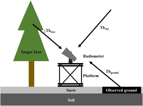
The SodRad (Sodankylä Radiometer) radiometer system was used for the in-situ ground based downward and upward-looking observations of the ground surface and forest vegetation at the intensive observation area (IOA) and forest. This radiometer operates at 10.65, 18.7, 21 and 36.5 GHz channels in both horizontal (H) and vertical (V) polarizations (pol) (see Lemmetyinen et al. 2016; Lemmetyinen et al. 2018). A mature Scots pine tree (Pinus sylvestris L.) about 15 m tall was selected as a specimen (target tree) representing forest conditions. The upwelling microwave Tb of the ground (Tb_ground), the downwelling Tb of the specimen tree (↓Tb_tree), and the downwelling Tb of the sky (Tb_sky) at 45° elevation were measured twice per day (one during daytime and one at night) from 5 Sep 2016 to 17 Apr 2017. Full experimental details can be found in Li et al. (2019) Figure 1.

Figure 1. The configuration of the radiometer observation experiment (Li et al. 2019).

Satellite-observed Tbs (Tb_AMSR) at 10.65, 18.7, 21 and 36.5 GHz in both H and V pol were obtained by the Advanced Microwave Scanning Radiometer 2 (AMSR2) (Okuyama and Imaoka 2015) from 1 Sept 2016 to 30 Apr. 2017. The descending passes were chosen since this is when the snow was likely to be below freezing. This study used the Level 1 resampled product (L1R) (Maeda, Taniguchi, and Imaoka 2016) with the footprints of the Tb_AMSR in all the frequencies resampled to 24 × 42 km ellipse (along scan × along track).

2.2.2. Ancillary data

Two automatic weather stations (AWS) were installed at the study site, one under the forest canopy and another is in the forest opening. The air temperature, the soil temperature, and the snow depth were measured every 10 min by the AWS. These AWS data were synchronized with the ground radiometer observations and spaceborne observation data. The AWS-measured snow depth in the forest (SD_forest) and forest opening (SD_open) was from a SR50 device. The forest and the forest opening sites are the two major landscape components in the AMSR2 footprint, the weighted average of SD_forest and SD_open was used to represent the snow depth of the AMSR2 footprint (SD_AMSR). SD_AMSR was calculated as $\mathrm{S}{\mathrm{D}}_{\mathrm{AMSR}}=f\ast \mathrm{S}{\mathrm{D}}_{\mathrm{forest}}+(1-f)\ast \mathrm{S}{\mathrm{D}}_{\mathrm{open}}$. The average value of these two AWS measured air temperatures at 2 meters above ground level were used to represent the overall air temperature of the study site (T_air). The soil temperature (T_ground) was measured at −5 cm depth in the forest opening.

To compare the tree skin temperature with the air temperature, two thermometers were installed at the bark-cambium interface of the target tree’s trunk, facing north at a height of 2.2 and 4.5 m. The temperature of the bark-cambium interface was measured in the interval of 10 min, and the averaged value of the two thermometers’ measurement is used to represent the tree skin temperature (T_tree).

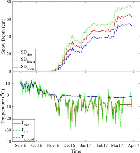
Figure 2 shows the snow depth and temperature information in the IOA. The first snowfall occurred on 28 Oct. 2016. The snow depth in the forest was about 70% of the snow depth in the forest opening. During the period that the ground was snow-free, T_air, T_ground and T_tree were similar with variable fluctuations, while during the period that the ground was covered by snow, T_ground was less variable, while T_air and T_tree fluctuated. The behavior of T_air and T_tree are very similar. The root mean square difference between T_air and T_tree is 2.34 K.

Figure 2. Time series of snow depth (upper panel) and environmental temperatures (lower panel) in IOA.

2.2.3. Forest emission modeling

The full details of this in-situ forest emission simulation can be found in the work of Li et al. (2019). Only a brief description is included in this section. This paper used many abbreviations. For the readability, these abbreviations are listed in the appendix.

Following the approach of Mätzler (1994), the upwelling emission observed above the forest cover ($\uparrow T{b}_{\mathrm{forest}}$) can be expressed by the radiative transfer (RT) equations below: (1) $\begin{array}{rl}\uparrow T{b}_{\mathrm{forest}}=& \gamma T{b}_{\mathrm{ground}}+(1-r_{\mathrm{forest}}-\gamma )T+(1-r_{\mathrm{forest}}-\gamma )r_{\mathrm{ground}}\gamma T\\ & +r_{\mathrm{forest}}T{b}_{\mathrm{sky}}+r_{\mathrm{ground}}{\gamma }^{2}T{b}_{\mathrm{sky}}\end{array}$(1) where $\gamma$ and $r_{\mathrm{forest}}$ are the transmissivity and the reflectivity of the forest vegetation layer respectively, $r_{\mathrm{ground}}$ is the reflectivity of the ground, $T$ is the temperature, $T{b}_{\mathrm{sky}}$ is the downwelling sky emission, and $T{b}_{\mathrm{ground}}$ is the upwelling ground emission. Since $r_{\mathrm{forest}}$ is relatively small, vegetation is treated as an attenuating layer as a commonly simplified approximation (see Jackson and Schmugge 1991; Njoku and Entekhabi 1996; Pulliainen and Grandeil 1999; Langlois et al. 2011) and $r_{\mathrm{forest}}$ is considered equal to 0. In thermal equilibrium, $r_{\mathrm{ground}}$ can be estimated by: (2) $r_{\mathrm{ground}}\approx 1-{\displaystyle \frac{T{b}_{\mathrm{ground}}}{T_{\mathrm{ground}}}}$(2) where $T_{\mathrm{ground}}$ is the ground soil temperature. The model developed by Li et al. (2020a) is applied to estimate tree transmissivity under sub-zero temperature conditions: $\gamma =1-{\displaystyle \frac{(1-{\gamma }_0)}{1-a_{\gamma }\ast T}T\le 0{}^{\circ }\mathrm{C}}$ (3) $\gamma ={\gamma }_{0}T>0{}^{\circ }\mathrm{C}$(3) where $a_{\gamma }$ is an empirical parameter, and ${\gamma }_0$ is the mean transmissivity of the forest layer measured when the air temperature is above 0°C. The parameter $a_{\gamma }$ and ${\gamma }_0$ have been determined by Li et al. (2020a) are presented in Table 1 for this site. As explained by Li et al. (2020a), the air temperature is easier to obtain during the operational snow retrieval than the tree skin temperature, and according to Figure 2, the value of T_air and T_tree are very similar. Therefore, $T$ is the air temperature instead of tree skin temperature, and $a_{\gamma }$ is estimated based on the value of T_air in this study.

Table 1. Estimated parameters, R², and the RMSE of transmissivity model.

	H10	V10	H18	V18	H21	V21	H37	V37
${\mathit{\gamma }}_0(-)$	0.23	0.24	0.18	0.19	0.15	0.14	0.13	0.12
${\mathit{a}}_{\mathit{\gamma }}$ (1/°C)	0.02	0.03	0.02	0.02	0.02	0.02	0.01	0.02

The RT model (1) is applied to the forest emission simulation. The in-situ measured values Tb_ground, Tb_sky, T_air, and T_ground are used as $T{b}_{\mathrm{ground}}$, $T{b}_{\mathrm{sky}}$, $T$, and $T_{\mathrm{ground}}$ in (1) and (2). $\gamma$ is estimated by (3), and $r_{\mathrm{ground}}$ is estimated by (2). With these inputs, the $\uparrow T{b}_{\mathrm{forest}}$ calculated by (1) is named as ↑Tb_RTforest. Details of this in-situ forest emission simulation can be found in the work of Li et al. (2020a).

2.2.4 An approximation of the influence of forest emission on spaceborne ΔTbs developed based on the in-situ forest emission simulation

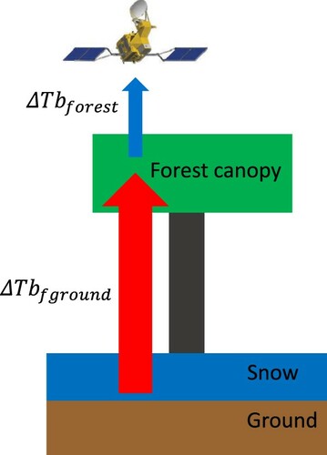
In forested areas, the ΔTb of the ground emission beneath the forest ($\mathrm{\Delta }T{b}_{\mathrm{fground}}$) is mainly used for PM SWE or SD retrievals. However, the ΔTb of the upwelling emission observed above the canopy ($\mathrm{\Delta }T{b}_{\mathrm{forest}}$) is that which is actually obtained by spaceborne or airborne instruments, as shown in Figure 3. Therefore, to reduce the influence of forest cover on the frequency difference PM snow retrieval algorithms $\mathrm{\Delta }T{b}_{\mathrm{fground}}$ should be estimated from $\mathrm{\Delta }T{b}_{\mathrm{forest}}$. As discussed, while forest RT models can be implemented for this purpose, to obtain the parameters required by the RT model is a challenge at the scale of satellite observations. Therefore, a simplified semi-empirical approximation is developed based on the result of in-situ forest emission simulations.

Figure 3. Schematic illustration of the influence of forest biomass on the observation of ground ΔTb.

In this approach, under sub-zero temperature conditions, the influence of the temperature-transmissivity relationship on $\mathrm{\Delta }T{b}_{\mathrm{fground}}$ is approximated by a linear equation $b\ast T+c$, where $T$ is the air temperature, and $b$ and $c$ are the empirical parameters to represent the influence of $T$ on $\mathrm{\Delta }T{b}_{\mathrm{fground}}$ through the temperature-transmissivity relationship. The approximation approach developed to describe the relationship between $\mathrm{\Delta }T{b}_{\mathrm{forest}}$, $\mathrm{\Delta }T{b}_{\mathrm{fground}}$, and $T$ is thus presented as: (4) $\mathrm{\Delta }T{b}_{\mathrm{forest}}=(b_{is}\ast T+c_{is})\ast \mathrm{\Delta }T{b}_{\mathrm{fground}}$(4) where $b_{is}$ and $c_{is}$ are the empirical parameters of this in-situ based forest emission simulation study.

For calibrating (4), the ΔTb of ↑Tb_RTforest (ΔTb_RTforest) is calculated by (1). By using the ΔTb_RTforest, T_air, and the radiometer observed ΔTb of Tb_ground to represent $\mathrm{\Delta }T{b}_{\mathrm{forest}}$, $T$, and $\mathrm{\Delta }T{b}_{\mathrm{fground}}$ in (4), $b_{is}$ and $c_{is}$are estimated by the least squares fitting method. Combinations of the Tb difference of the channels 10.65 - 36.5 GHz V pol (10-37 V) and 18.7 - 36.5 GHz V pol (18-37 V) were studied. The results are presented in Table 3 in the Results section.

With the estimated $b_{is}$ and $c_{is}$, the $\mathrm{\Delta }T{b}_{\mathrm{forest}}$ approximation in (4) is now denoted as ΔTb_APPforest. In this study, based on the AWS measured T_air, ΔTb_APPforest was simulated with $\mathrm{\Delta }T{b}_{\mathrm{fground}}$ values of 10, 20, 30, 40, and 50 K by (4). In Figure 6, ΔTb_APPforest is compared with ΔTb_RTforest.

To demonstrate the potential of this approximation in the spaceborne application, a simple test was made using AMSR2 observations to demonstrate how this approach could be applied to reduce the influence of temperature-transmissivity relationship on spaceborne observed ΔTb. The scene of a snow covered AMSR2 footprint was simplified into two main elements: forest and forest opening. Accordingly, the ΔTb of the spaceborne observation ($\mathrm{\Delta }T{b}_{sb}$) is expressed below: (5) $\mathrm{\Delta }T{b}_{sb}=f\ast \mathrm{\Delta }T{b}_{\mathrm{forest}}+(1-f)\ast \mathrm{\Delta }T{b}_{\mathrm{oground}}$(5) where $\mathrm{\Delta }T{b}_{\mathrm{forest}}$ is the ΔTb of the upwelling emission above the canopy in the forest region, $\mathrm{\Delta }T{b}_{\mathrm{oground}}$ is the ΔTb of the ground emission in the forest openings, and $f$ is the percentage of the forest fraction. As explained, $f$ = 0.55.

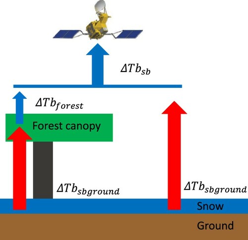
For convenience, we followed the approach of Langlois et al. (2011), assuming the ground conditions in the forest region and in the forest opening to be similar. The variable $\mathrm{\Delta }T{b}_{\mathrm{sbground}}$ represents the overall ΔTb of sub-canopy ground emission from the spaceborne AMSR2 observation footprint as shown in Figure 4. Accordingly, $\mathrm{\Delta }T{b}_{\mathrm{sbground}}=\mathrm{\Delta }T{b}_{\mathrm{oground}}=\mathrm{\Delta }T{b}_{\mathrm{fground}}$. Equation (5) can therefore be re-written as: (6) $\mathrm{\Delta }T{b}_{sb}=f\ast (b_{sb}\ast T+c_{sb})\ast \mathrm{\Delta }T{b}_{\mathrm{sbground}}+(1-f)\ast \mathrm{\Delta }T{b}_{\mathrm{sbground}}$(6) where $b_{sb}$ and $c_{sb}$ are the empirical parameters for the spaceborne observation. By re-arranging (6), $\mathrm{\Delta }T{b}_{\mathrm{sbground}}$ can be estimated through $\mathrm{\Delta }T{b}_{sb}$. As explained, $\mathrm{\Delta }T{b}_{\mathrm{sbground}}$ is the value theoretically independent of the forest cover. Therefore, using $\mathrm{\Delta }T{b}_{\mathrm{sbground}}$ instead of $\mathrm{\Delta }T{b}_{sb}$ in the spaceborne snow retrieval procedure, we can reduce the influence of forest emission on passive microwave snow retrieval in forested terrain.

Figure 4. Schematic illustration of terms in Equation (6).

For estimating the empirical parameter $b_{sb}$ and $c_{sb}$ in this study, the values of $\mathrm{\Delta }T{b}_{\mathrm{sbground}}$, $\mathrm{\Delta }T{b}_{sb}$ and T are needed to calibrate (6). The values of $\mathrm{\Delta }T{b}_{sb}$ and T were obtained from AMSR2 Tb data and the AWS air temperature data respectively. For $\mathrm{\Delta }T{b}_{\mathrm{sbground}}$, because the radiometer only observed the ground emission in the forest opening, this observation cannot be used directly. Therefore, a polynomial regression model between the ΔTb of the ground emission ($\mathrm{\Delta }T{b}_{\mathrm{ground}}$) and the snow depth ($SD$) is established based on the radiometer observations Tb and the snow depth: (7) $\mathrm{\Delta }T{b}_{\mathrm{ground}}=d\ast S{D}^2+e\ast SD$(7) where the $c$ and $d$ are the regression coefficients. Equation (7) was calibrated by the least squares fitting method based on SD_open and the ΔTb of the radiometer observed Tb_ground in the forest opening. Results of the calibrated Equation (7) are shown in Figure 5 with Equation (7) as a solid lines and radiometer observations of ΔTb of Tb_ground as blue–green-red circle markers. The blue–green-red color bar represents coincident air temperature. Table 2 shows the fitting parameters $d$ and $e$, R² and the RMSE.

Figure 5. Radiometer-observed ΔTb of Tb_ground (blue-green-red circle markers) with the (7) simulated results (black solid lines), the blue-green-red bar represents T_air.

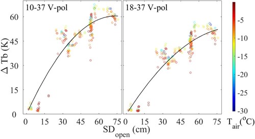
Table 2. Estimated parameters, R², and RMSE of Equation (7).

	$\mathit{d}$ (K/cm^2)	$\mathit{e}$ (K/cm)	R^2	RMSE (K)
10-37 V-pol	−0.011	1.64	0.87	6.50
18-37 V-pol	−0.0064	1.18	0.85	6.68

This very localized ground ΔTb estimation approach (Equation (7)) can be applied in a very limited region, but it can be deployed by a more generally applicable modeling approach [see HUT (Pulliainen and Grandeil 1999), MEMLS (Wiesmann and Mätzler 1999), and DMRT (Tsang et al. 2006; Picard et al. 2013)] for future applications. It is also independent of snow on tree canopy, which according to the work of Li et al. (2019), has negligible influence on tree emission in this study although, under different climate conditions, the tree canopy snow may have a stronger influence.

With (7) calibrated, $\mathrm{\Delta }T{b}_{\mathrm{sbground}}$ can be estimated with SD_AMSR. In (6), the ΔTb of Tb_AMSR (ΔTb_AMSR) is used as $\mathrm{\Delta }T{b}_{sb}$, and T_air is used as $T$, with $b_{sb}$ and $c_{sb}$ estimated by a least squares fit. The results are presented in Table 4.

Since (6) has been calibrated, the $\mathrm{\Delta }T{b}_{sb}$ simulated by this approximation approach is named as ΔTb_APPsb. ΔTb_APPsb was simulated by Equations (6) and (7) at the $SD$ equal to 10, 25, 40, 55, and 70 cm based on the value of T_air and $f$. In Figure 7, ΔTb_APPsb is compared with ΔTb_AMSR.

In this paper, as a case study, $\mathrm{\Delta }T{b}_{\mathrm{sbground}}$ in Sodankylä is calculated based on the ΔTb_AMSR and T_air by the re-arranged Equation (6). The $\mathrm{\Delta }T{b}_{\mathrm{sbground}}$ calculated by this approximation approach (6) is named as ΔTb_APPsbground. To demonstrate how Equation (6) could reduce the influence of the forest on the ground ΔTbs, ΔTb_APPsbground and ΔTb_AMSR are compared with the radiometer observed ΔTb of Tb_ground in Figure 9.

For validating this approximation approach developed in Sodankylä, this approach was also applied in Enontekiö Näkkälä (Lat/Lon: 68.6/23.58, forest fraction: 24.6%) and Salla Naruska (Lat/lon: 67.16/29.18, forest fraction: 67.0%) in the Lapland region. The AMSR2 observed Tb from 1 Sep 2016 to 31 May 2017 is used. The snow depth and air temperature is obtained from the Global Surface Summary of the Day (GSOD) dataset (WMO station number: 2726 and 2745).

3. Results

In Figure 6, ΔTb model and approximation values for 10-36 V and 18-36 V are shown. Colored circles denote the RT model estimates from Equation (1) that simulate ΔTb_RTforest, and the colored lines show the simplified approximation approach from Equation (4) that simulate ΔTb_APPforest. ΔTb_APPforest was simulated with values of $\mathrm{\Delta }T{b}_{fground}$ = 10, 20, 30, 40, and 50 K in (4). Because ΔTb_RTforest is calculated based on the radiometer observed ground Tb in the forest opening, the blue–green-red bar represents SD_open. According to Figure 6, the ΔTb_RTforest and ΔTb_APPforest is influenced by both the air temperature and the snow depth. ΔTb_RTforest with a deeper snow depth has a higher sensitivity to the air temperature. This is because as the snow depth increases, the ΔTb of the ground emission also tends to increase (as Figure 5 shows). Table 3 presents the estimated parameters and the goodness of fit of equation (4)(4) $\mathrm{\Delta }T{b}_{\mathrm{forest}}=(b_{is}\ast T+c_{is})\ast \mathrm{\Delta }T{b}_{\mathrm{fground}}$(4) during the model calibration between ΔTb_RTforest, T_air, and the radiometer observed ΔTb of Tb_ground.

Figure 6. Comparison between ΔTb_RTforest (blue-green-red circle markers) and ΔTb_APPforest which is simulated at $\mathrm{\Delta }T{b}_{fground}$ equal to 10, 20, 30, 40, and 50 K by (4) (lines), the blue-green-red bar represents SD_open.

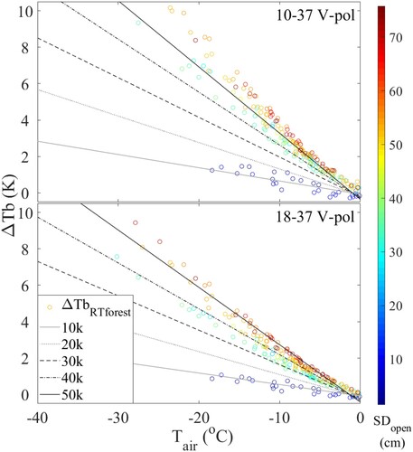
Table 3. Estimated parameters b_is and c_is, and corresponding R2, and RMSE of (4) against RT model (1) for the model calibration.

	${\mathit{b}}_{\mathit{i}s}$ (1/°C)	${\mathit{c}}_{\mathit{i}s}$ (-)	R^2	RMSE (K)
10-37 V-pol	−0.0073	−0.0071	0.99	0.29
18-37 V-pol	−0.0063	−0.0084	0.99	0.18

According to Figure 6 and Table 3, the approximation approach (ΔTb_APPforest) has a good agreement with the RT model simulations (ΔTb_RTforest). This result indicates that the approximation [Equation (4)] developed is applicable as a simplified method to parameterize the influence of forests on ground ΔTbs.

In Figure 7, the approximation approach from Equation (6) is applied to the spaceborne AMSR2 data. ΔTb_AMSR (the AMSR2 observed ΔTb) is represented by the colored circles, and ΔTb_APPsb (the simulated ΔTb in AMSR2 footprint) is represented by the lines. ΔTb_APPsb was simulated by (6) and (7) for $SD$ set to 10, 25, 40, 55, and 70 cm. In Figure 7, the y-axis represents the ΔTb value of ΔTb_AMSR and ΔTb_APPsb, the x-axis represents T_air. Because ΔTb_AMSR and ΔTb_APPsb are the ΔTb in AMSR footprint, the blue–green-red bar in Figure 7 represents SD_AMSR. Figure 7 shows that the ΔTb_AMSR and ΔTb_APPsb are sensitive to both air temperature and the snow depth, which is comparable to the ΔTb_RTforest and ΔTb_APPforest in Figure 6. For non-forested areas within AMSR2 footprints, only snow depth influences the ground ΔTb. Therefore, compared with ΔTb_RTforest and ΔTb_APPforest which are simulated in a full forest covered condition, ΔTb_AMSR and ΔTb_APPsb have a higher sensitivity to the snow depth, and a lower sensitivity to the air temperature. Table 4 shows the estimated parameters and the goodness of fit of Equation (6) during the model calibration between ΔTb_AMSR, T_air, and SD_AMSR.

Figure 7. Comparison between ΔTb_AMSR (blue-green-red circle markers) and ΔTb_APPsb which is simulated at snow depths equal to 10, 25, 40, 55, and 70 cm (lines), the blue-green-red bar represents SD_AMSR.

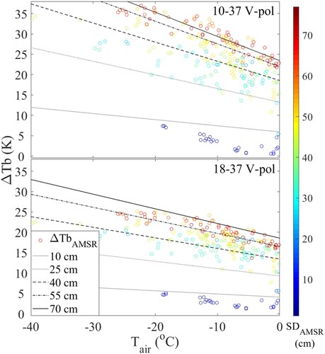
Table 4. The estimated parameters b_sb and c_sb, and the corresponding R2, and RMSE of (6) against ΔTb_AMSR during the model calibration with training dataset.

	${\mathit{b}}_{\mathit{s}b}$ (1/°C)	${\mathit{c}}_{\mathit{s}b}$ (-)	R^2	RMSE (K)
10-37 V-pol	−0.019	−0.088	0.85	3.41
18-37 V-pol	−0.014	−0.13	0.75	2.96

According to Figure 7 and Table 4, the ΔTb_APPsb has a good agreement with ΔTb_AMSR, indicating that the approximation approach developed in this study can be used to simulate how the forest cover influences the ΔTb of the ground emission observed by spaceborne Tbs. Therefore, the re-arranged approximation approach (6) can be applied to reduce the influence of forest emission on spaceborne-observed ΔTb.

Figure 8 presents ΔTb_APPsbground calculated from the re-arranged approximation approach (6) based on ΔTb_AMSR, T_air, and SD_AMSR. As discussed, ΔTb_APPsbground can be considered as an estimate of the ground ΔTb without the influence of the forest. As Figure 8 shows, ΔTb_APPsbground is not influenced by T_air, unlike ΔTb_AMSR in Figure 7. In Figure 8, the y-axis represents the value of ΔTb_APPsbground, the x-axis represents T_air, and the blue–green-red bar represents SD_AMSR.

Figure 8. ΔTb_APPsbground (blue-green-red circle markers) against T_air, the blue-green-red bar represents SD_AMSR.

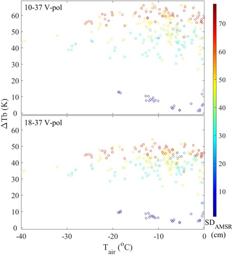
Finally, in Figure 9, we show ΔTb_APPsbground (blue–green-red circles in panels (a) and (b)) and ΔTb_AMSR (blue–green-red circles in panels (c) and (d)) as a function of snow depth and air temperature. The radiometer observed ΔTb of Tb_ground are shown as black crosses. For the radiometer observed ΔTb of Tb_ground, because the radiometer ground observation made in the forest opening, the Tbs only be influenced by SD_open. Therefore, the x-axis represents SD_open for this data set in Figure 9. While for ΔTb_APPsbground and ΔTb_AMSR, they are the simulation and observation in AMSR2 footprint. The Tbs are influence by the snow depth in the whole AMSR observation footprint instead of the snow depth in forest open. Therefore, x-axis represents SD_AMSR for these data set.

Figure 9. Compared ΔTb_APPsbground (blue-green-red circle markers in (a) and (b)) and ΔTb_AMSR (blue-green-red circle markers in (c) and (d)) with the radiometer observed ΔTb of Tb_ground (black cross markers), the blue-green-red bar represents T_air.

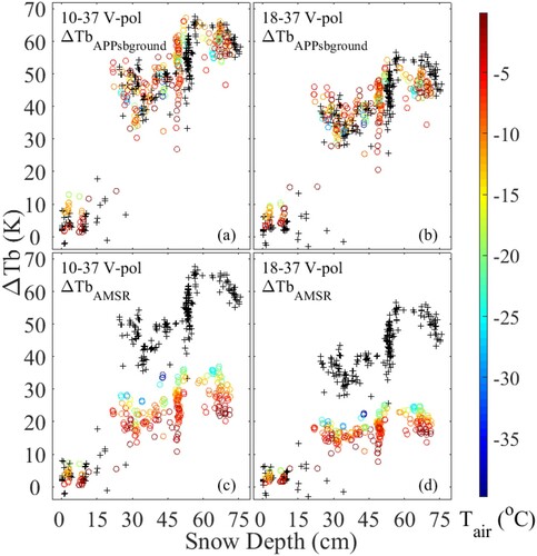
Comparing ΔTb_APPsbground with ΔTb_AMSR, ΔTb_APPsbground is not influenced by the air temperature, and has a greater sensitivity to the snow depth. Comparing ΔTb_APPsbground and ΔTb_AMSR with the radiometer-observed ΔTb of Tb_ground, ΔTb_APPsbground has a higher similarity with the ΔTb of Tb_ground. According to Figure 5, the ΔTb of Tb_ground is not sensitive to air temperature. As discussed, the temperature-transmissivity relationship causes the ΔTb_AMSR to be sensitive to air temperature under sub-zero temperatures. The results of this comparison indicate that the influence the temperature-transmissivity relationship of the forest on the AMSR2 observed ΔTb is reduced in ΔTb_APPsbground by the approximation approach developed in this paper.

4. Validation

The RMSE between the AMSR2 observed ΔTb and the Equation (6) simulated ΔTb in Enontekiö Näkkälä and Salla Naruska are 8.82 and 4.57 K respectively, which indicates that the approximation approach has a good performance at these two locations. In Figure 10, the simulated ΔTb in AMSR2 footprint (ΔTb_APPsb) is compared with the AMSR2 observed data (ΔTb_AMSR). The ΔTb_APPsb is simulated at the snow depth of 10, 25, 40, 55, and 70 cm by the Equation (6) with the parameters estimated in Sodankylä (Table 4). The ΔTb_AMSR is represented by blue–green-red circle markers. The blue–green-red bar represents the snow depth in GSOD dataset.

Figure 10. Comparison between ΔTb_AMSR (blue-green-red circle markers) and ΔTb_APPsb which is simulated at snow depths equal to 10, 25, 40, 55, and 70 cm (lines), the blue-green-red bar represents SD_AMSR.

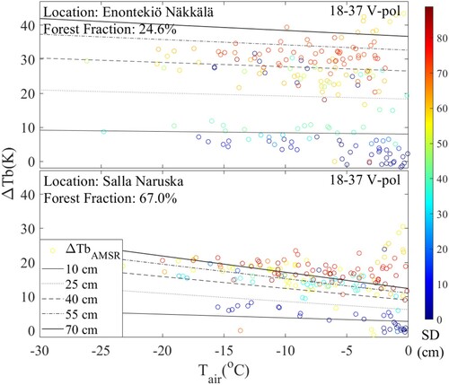
Salla Naruska has a higher forest fraction than Enontekiö Näkkälä. Therefore, the temperature-transmissivity relationship should have a higher influence on the ΔTb in Salla Naruska. According to Figure 10, the ΔTb in Salla Naruska has a higher sensitivity to the temperature, which indicated that the forest has a higher influence on ΔTb in Salla Naruska. Both the observed and the simulated results have shown this tendency.

In Figure 11, ΔTb_AMSR in (c) and (d) are the AMSR2 observed ΔTb in Enontekiö Näkkälä and Salla Naruska. While, ΔTb_APPsbground in (a) and (b) are the ΔTb_AMSR corrected by the re-arranged approximation approach (6). Both ΔTb_AMSR and ΔTb_APPsbground are compared with the SodRod radiometer in-situ observed brightness temperature in Sodankylä (ΔTb_ground). The blue–green-red bar represents the air temperature in GSOD dataset.

Figure 11. Compared ΔTb_APPsbground (blue-green-red circle markers in (a) and (b)) and ΔTb_AMSR (blue-green-red circle markers in (c) and (d)) with the radiometer observed ΔTb of Tb_ground (black cross markers), the blue-green-red bar represents T_air.

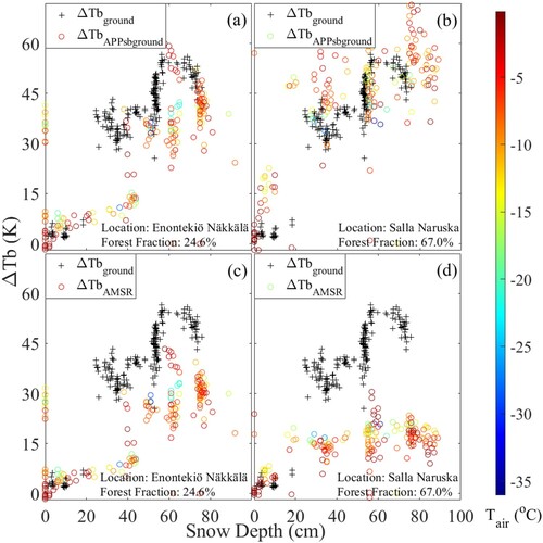
The results in Figure 11 is very similar as the result in Figure 9. Comparing ΔTb_APPsbground with ΔTb_AMSR, ΔTb_APPsbground has a higher similarity with the in-situ radiometer observed ΔTb, and has a greater sensitivity to the snow depth. The results indicate that the influence of the temperature-transmissivity relationship on the AMSR2 observed ΔTb in Enontekiö Näkkälä and Salla Naruska is reduced by the approximation approach.

5. Discussion

The temperature-transmissivity relationship, first reported by Li et al. (2019), indicated that the sensitivity of ΔTb to the ground SD and SWE increases in a forest environment as air temperatures decrease below sub-zero temperature conditions (Li et al. 2020a). When observed by aircraft or satellite radiometers the ΔTb above the forest canopy is influenced by both air temperature and the ΔTb of the ground emission underneath the forest under sub-zero temperature conditions (see Figures 6 and 7). The strong influence of the air temperature on the ΔTb explains why a constant adjustment coefficient approach (see Chang, Foster, and Hall 1996; Foster et al. 2005) is insufficient to correct the influence of forest attenuation on PM snow retrievals. This may also have contributed to differing parameterizations of forest microwave transmissivity obtained in previous studies (Cohen et al. 2015; Kruopis 1999; Langlois et al. 2011).

The soil condition is another factor could influence the ΔTb of the ground. The soil frozen causes the soil dielectric constant decrease, thereby the ΔTb of the ground decreases (Zhao et al. 2011). However, in this study, the temperature and the dielectric constant of the soil are relatively stable after the ground is covered by snow, the AWS measured results are presented in Li (2020b). Since this study focused on the snow covered ground, the soil condition has a limited influence on the ground ΔTb during winter time in this study.

According to Figures 8 and 9, ΔTb_APPsbground is not influenced by air temperature, unlike ΔTb_AMSR. Furthermore, ΔTb_APPsbground has a stronger sensitivity to the snow depth than ΔTb_AMSR. Compared with ΔTb_AMSR, the behavior of ΔTb_APPsbground with respect to the air temperature and snow depth has a higher similarity with the behavior of the ground-based radiometer observed ΔTb of Tb_ground. This result indicates that the approximation approach (Equation (6)) developed in this paper can effectively reduce the influence from both the forest attenuation effect (Foster et al. 2005) and the temperature-transmissivity relationship (Li et al. 2019; Li et al. 2020a) on the spaceborne or airborne observed ΔTb during snow retrievals.

Comparing Table 3 with Table 4, and despite the different data sources in calibrating (4) and (6), the coefficients b_is and c_is are remarkably similar in magnitude to b_sb and c_sb, given the many orders of magnitude difference in the spatial scales to which these apply. The differences between the in-situ and spaceborne b and c coefficients may be due to the different observation scale (the local single tree observation vs. the satellite scale observation), the biomass density difference between a single tree and a forest, and other land uses that are within the AMSR2 footprint that are not accounted for in this simple analysis. In addition, differences in the viewing geometries of the radiometers and the actual snow depth in the AMSR2 footprint from SD_AMSR also likely contribute to the differences in the coefficients. The negative values of the c coefficients imply a change of sign of the brightness difference from below the canopy to above the canopy as the air temperature approaches freezing, which is not expected from the physics of the problem, nor from the measurements we have. However, the differential canopy transmissivity is negative only for a few degrees Celsius, at most, below freezing. If we consider these to be fitting parameters for a more complex differential canopy transmissivity for which (4) and (6) are the first order Taylor series, we can see that this may simply be a result of fitting errors for this particular forest due to the approximations inherent in the form of (4) and (6).

In addition to the vegetation permittivity, the structure of the forest medium (e.g. density, stem volume, and height) also has a strong influence on the ΔTb. The pattern of the forest structure variation relates to the spatial scale of the observation (Smith and Urban 1988; Larue et al. 2017; Löfman and Kouki 2003; Shugart, Saatchi, and Hall 2010). At a small spatial scale of observation (at the scales which forest gaps can be observed), the period of the forest succession, disturbance and recovery can be observed. Therefore, the structure of a mature forest ecosystem is a heterogeneous mixture of patches at this scale. However, at a larger observation scale, like the AMSR2 observation, only the aggregated pattern can be observed, the heterogeneous nature of the forest spatial variability at the local scale has a limited influence on large scale observations. The structure of the forest stand is largely controlled by the climatic factors such as temperature and precipitation (Smith and Urban 1988; López-Serrano et al. 2005, Wang et al. 2006, Shugart, Saatchi, and Hall 2010; Pan et al. 2013) at this observation scale. Therefore, the structure of the forest stands is relatively consistent within the same biome (Holdridge 1967; Sitch et al. 2008; Wang et al. 2006).

In Equation (6), although the forest fraction has been considered, the variation of the forest structure has not been discussed yet. The forest structure should have a strong influence on the equation parameter $b$ and $c$. In this paper, the study sites are located inside the same biome. Therefore, the parameters $b$ and $c$ should be relatively consistent within the same biome. The validation in Enontekiö Näkkälä and Salla Naruska also support this argument. However, if this approach is needed to be applied over a different biome with a different forest structure, the influence of the forest structure on parameters $b$ and $c$ should be further evaluated. Maybe a lookup table could be developed to determine the parameters for different types of forest.

6. Conclusion

The permittivity variation caused by the cold temperature has a significant influence on the tree microwave radiative transfer (Li et al. 2019). Therefore, this phenomenon is an important factor in passive microwave passive microwave snow retrieval (Li et al. 2020a). However, this phenomenon has not been considered by current snow retrieval algorithms. A feasible correction approach is required.

For correcting the influence of this phenomenon on snow retrieval, simplified approximation was developed in this study to describe how the temperature-transmissivity relationship influences ΔTb in a forested region. This approximation approach has been evaluated over the study sites in Sodankylä, Enontekiö Näkkälä, and Salla Naruska. The results of the evaluation have demonstrated that this approximation approach has a strong potential to reduce the influence of the forest on the performance of the PM frequency difference snow retrieval algorithms. Therefore, it is recommended that this approximation should be evaluated more widely and adopted for and global scale PM snow retrievals in the future.

Acknowledgments

The ground measured radiometer data and ancillary data are provided by the FMI Arctic Research Centre, the GCOM-W1 AMSR2 level 1R Tb product is provided by JAXA, and MODIS MOD44b Version 6 Vegetation Continuous Field product data is provided by NASA EOSDIS Land Processes DAAC.

Disclosure statement

No potential conflict of interest was reported by the author(s).

Additional information

Funding

The research leading to these results has received fundings from Japan Aerospace Exploration Agency [contract number 20RT000300], the National Key Research and Development Program of China [grant number 2017YFE0111700], the NSERC Discovery Grant [grant number RGPIN-2017-04385], and INTERACT (International Network for Terrestrial Research and Monitoring in the Arctic) under the European Union H2020 Grant Agreement [grant number 730938].

Appendix

The abbreviations used in this paper.

Table

Variables of equations	Descriptions	Equation numbers	Measured data	Descriptions
$\uparrow T{b}_{\mathrm{forest}}$	Upwelling emission observed above the forest cover	(1)	Tbground	Radiometer measured ground Tb
$T{b}_{\mathrm{ground}}$	Upwelling ground emission	(1)(2)	↓Tbtree	Radiometer measured downwelling Tb of the specimen tree
$T{b}_{\mathrm{sky}}$	Downwelling sky emission	(1)	Tbsky	Radiometer measured downwelling Tb of the sky
$T$	Air temperature	(1)(3)(4)(6)	TbAMSR	Satellite-observed Tbs
$\gamma$	Transmissivity of the forest	(1)(3)	SDforest	AWS measured snow depth in the forest
$r_{\mathrm{forest}}$	Reflectivity of the forest	(1)	SDopen	AWS measured snow depth in the forest opening
$r_{\mathrm{ground}}$	Reflectivity of the ground	(1)(2)	Tair	The air temperature measured at IOA
$T_{\mathrm{ground}}$	Ground soil temperature	(2)	Tground	The soil temperature measured at IOA
$a_{\gamma }$	Empirical parameter	(3)	Ttree	The measured tree skin temperature
${\gamma }_0$	Mean transmissivity of the forest layer measured when the air temperature is above 0 °C	(3)	Calculated Data	Descriptions
			SDAMSR	The AWS measured snow depth of the AMSR2 footprint (Section 2.2.2, paragraph 1)
$\mathrm{\Delta }T{b}_{\mathrm{forest}}$	ΔTb of the upwelling emission observed above the canopy	(4)(5)	↑TbRTforest	$\uparrow T{b}_{\mathrm{forest}}$ calculated by the equation (1)
$\mathrm{\Delta }T{b}_{\mathrm{fground}}$	ΔTb of the ground emission beneath the forest	(4)	ΔTbRTforest	The ΔTb calculated based on ↑TbRTforest
$b_{is}$	Empirical parameter	(4)	ΔTbAPPforest	$\mathrm{\Delta }T{b}_{\mathrm{forest}}$ estimated by the equation (4)
$c_{is}$	Empirical parameter	(4)	ΔTbAPPsb	the $\mathrm{\Delta }T{b}_{sb}$ estimated by the equation (6)
$\mathrm{\Delta }T{b}_{sb}$	ΔTb of the spaceborne observation	(5)(6)	ΔTbAMSR	the ΔTb of TbAMSR
$\mathrm{\Delta }T{b}_{\mathrm{oground}}$	ΔTb of the ground emission in the forest openings	(5)	ΔTbAPPsbground	$\mathrm{\Delta }T{b}_{\mathrm{sbground}}$ estimated based on the ΔTbAMSR and Tair by the re-arranged equation (6)
$f$	Forest coverage	(5)(6)
$\mathrm{\Delta }T{b}_{\mathrm{sbground}}$	The overall ΔTb of sub-canopy ground emission from the spaceborne AMSR2 observation footprint	(6)
$b_{sb}$	Empirical parameter	(6)
$c_{sb}$	Empirical parameter	(6)
$\mathrm{\Delta }T{b}_{\mathrm{ground}}$	ΔTb of the ground emission	(7)
$SD$	Snow depth	(7)
$c$	Regression coefficient	(7)
$d$	Regression coefficient	(7)

References

- Chang, A. T. C., J. L. Foster, and D. K. Hall. 1996. “Effects of Forest on the Snow Parameters Derived from Microwave Measurements During the BOREAS Winter Field Campaign.” Hydrological Processes 10 (12): 1565–1574.
- Cohen, Juval, Juha Lemmetyinen, Jouni Pulliainen, Kirsikka Heinila, Francesco Montomoli, Jaakko Seppanen, and Martti T. Hallikainen. 2015. “The Effect of Boreal Forest Canopy in Satellite Snow Mapping-A Multisensor Analysis.” IEEE Transactions on Geoscience and Remote Sensing 53 (12): 6593–6607.
- Derksen, Chris. 2008. “The Contribution of AMSR-E 18.7 and 10.7 GHz Measurements to Improved Boreal Forest Snow Water Equivalent Retrievals.” Remote Sensing of Environment 112 (5): 2701–2710.
- Foster, James L., Chaojiao Sun, Jeffrey P. Walker, Richard Kelly, Alfred Chang, Jiarui Dong, and Hugh Powell. 2005. “Quantifying the Uncertainty in Passive Microwave Snow Water Equivalent Observations.” Remote Sensing of Environment 94 (2): 187–203.
- Holdridge, L. R. 1967. Life Zone Ecology. San José. Costa Rica: Tropical Science Center.
- Jackson, T. J., and T. J. Schmugge. 1991. “Vegetation Effects on the Microwave Emission of Soils.” Remote Sensing of Environment 36 (3): 203–212.
- Kelly, Richard E. 2009. “The AMSR-E Snow Depth Algorithm: Description and Initial Results.” Journal of the Remote Sensing Society of Japan 29 (1): 307–317.
- Kelly, Richard E., Alfred T. Chang, Leung Tsang, and James L. Foster. 2003. “A Prototype AMSR-E Global Snow Area and Snow Depth Algorithm.” IEEE Transactions on Geoscience and Remote Sensing 41 (2): 230–242.
- Kelly, Richard E., Qinghuan Li, and Nastaran Saberi. 2019. “The AMSR2 Satellite-Based Microwave Snow Algorithm (SMSA): A New Algorithm for Estimating Global Snow Accumulation.” In International Geoscience and Remote Sensing Symposium (IGARSS). https://doi.org/https://doi.org/10.1109/IGARSS.2019.8898525.
- Kou, Xiaokang, Linna Chai, Lingmei Jiang, Shaojie Zhao, and Shuang Yan. 2015. “Modeling of the Permittivity of Holly Leaves in Frozen Environments.” IEEE Transactions on Geoscience and Remote Sensing. doi:https://doi.org/10.1109/TGRS.2015.2431495.
- Kruopis, Nerijus. 1999. “Passive Microwave Measurements of Snow-Covered Forest Areas in Em Ac’95.” IEEE Transactions on Geoscience and Remote Sensing. doi:https://doi.org/10.1109/36.803417.
- Langlois, Alexandre, Alain Royer, Florent Dupont, Alexandre Roy, Kalifa Goita, and G. Picard. 2011. “Improved Corrections of Forest Effects on Passive Microwave Satellite Remote Sensing of Snow Over Boreal and Subarctic Regions.” IEEE Transactions on Geoscience and Remote Sensing. doi:https://doi.org/10.1109/TGRS.2011.2138145.
- Larue, Fanny, Alain Royer, Danielle De Sève, Alexandre Langlois, Alexandre Roy, and Ludovic Brucker. 2017. “Validation of GlobSnow-2 Snow Water Equivalent Over Eastern Canada.” Remote Sensing of Environment. doi:https://doi.org/10.1016/j.rse.2017.03.027.
- Lemmetyinen, J., A. Kontu, L. Leppänen, J. Vehviläinen, R. Vehmas, Qinghuan Li, K. Rautiainen, and J. Pulliainen. 2018.. “Season -Length Observations of Active and Passive Microwave Signatures of Snow Cover in a Boreal Forest Environment.” In International Geoscience and Remote Sensing Symposium (IGARSS). Vol. 2018-July. https://doi.org/https://doi.org/10.1109/IGARSS.2018.8517328.
- Lemmetyinen, Juha, Anna Kontu, Jouni Pulliainen, Juho Vehviläinen, Kimmo Rautiainen, Andreas Wiesmann, Christian Mätzler, et al. 2016. “Nordic Snow Radar Experiment.” Geoscientific Instrumentation, Methods and Data Systems. doi:https://doi.org/10.5194/gi-5-403-2016.
- Li, Qinghuan. 2020b. “The Influence of Winter Time Boreal Forest Tree Transmissivity on Tree Emission and Passive Microwave Snow Observations.” Doctoral Dissertation, Waterloo, ON: University of Waterloo.
- Li, Qinghuan, and R. E. J. Kelly. 2017. “Correcting Satellite Passive Microwave Brightness Temperatures in Forested Landscapes Using Satellite Visible Reflectance Estimates of Forest Transmissivity.” IEEE Journal of Selected Topics in Applied Earth Observations and Remote Sensing 10 (9). doi:https://doi.org/10.1109/JSTARS.2017.2707545.
- Li, Qinghuan, R. E. J. Kelly, J. Lemmetyinen, and J. Pan. 2020a. “Simulating the Influence of Temperature on Microwave Transmissivity of Trees During Winter Observed by Spaceborne Microwave Radiometery.” IEEE Journal of Selected Topics in Applied Earth Observations and Remote Sensing. doi:https://doi.org/10.1109/JSTARS.2020.3017618.
- Li, Qinghuan, R. E. J. Kelly, L. Leppanen, J. Vehvilainen, A. Kontu, J. Lemmetyinen, and J. Pulliainen. 2019. “The Influence of Thermal Properties and Canopy-Intercepted Snow on Passive Microwave Transmissivity of a Scots Pine.” IEEE Transactions on Geoscience and Remote Sensing 57 (8). doi:https://doi.org/10.1109/TGRS.2019.2899345.
- Löfman, Satu, and Jari Kouki. 2003. “Scale and Dynamics of a Transforming Forest Landscape.” Forest Ecology and Management. doi:https://doi.org/10.1016/S0378-1127(02)00133-0.
- López-Serrano, F. R., A. García-Morote, M. Andrés-Abellán, A. Tendero, and A. Del Cerro. 2005. “Site and Weather Effects in Allometries: A Simple Approach to Climate Change Effect on Pines.” Forest Ecology and Management. doi:https://doi.org/10.1016/j.foreco.2005.05.014.
- Luojus, K., J. Pulliainen, M. Takala, et al. 2013. GlobSnow-2 Product User Guide Version 1.0. Paris: European space agency.
- Maeda, Takashi, Yuji Taniguchi, and Keiji Imaoka. 2016. “GCOM-W1 AMSR2 Level 1R Product: Dataset of Brightness Temperature Modified Using the Antenna Pattern Matching Technique.” IEEE Transactions on Geoscience and Remote Sensing. doi:https://doi.org/10.1109/TGRS.2015.2465170.
- Mätzler, C. 1994. “Microwave Transmissivity of a Forest Canopy: Experiments made with a Beech.” Remote Sensing of Environment 48 (2): 172–180.
- Njoku, Eni G., and Dara Entekhabi. 1996. “Passive Microwave Remote Sensing of Soil Moisture.” Journal of Hydrology. doi:https://doi.org/10.1016/0022-1694(95)02970-2.
- Okuyama, Arata, and Keiji Imaoka. 2015. “Intercalibration of Advanced Microwave Scanning Radiometer-2 (AMSR2) Brightness Temperature.” IEEE Transactions on Geoscience and Remote Sensing. doi:https://doi.org/10.1109/TGRS.2015.2402204.
- Pan, Yude, Richard A. Birdsey, Oliver L. Phillips, and Robert B. Jackson. 2013. “The Structure, Distribution, and Biomass of the World’s Forests.” Annual Review of Ecology, Evolution, and Systematics. doi:https://doi.org/10.1146/annurev-ecolsys-110512-135914.
- Pan, Jinmei, Michael Durand, Melody Sandells, Juha Lemmetyinen, Edward J. Kim, Jouni Pulliainen, Anna Kontu, and Chris Derksen. 2016. “Differences Between the HUT Snow Emission Model and MEMLS and Their Effects on Brightness Temperature Simulation.” IEEE Transactions on Geoscience and Remote Sensing. doi:https://doi.org/10.1109/TGRS.2015.2493505.
- Picard, G., L. Brucker, A. Roy, F. Dupont, M. Fily, A. Royer, and C. Harlow. 2013. “Simulation of the Microwave Emission of Multi-Layered Snowpacks Using the Dense Media Radiative Transfer Theory: The DMRT-ML Model.” Geoscientific Model Development. doi:https://doi.org/10.5194/gmd-6-1061-2013.
- Pulliainen, Jouni T., and Jochen Grandeil. 1999. “HUT Snow Emission Model and Its Applicability to Snow Water Equivalent Retrieval.” IEEE Transactions on Geoscience and Remote Sensing. doi:https://doi.org/10.1109/36.763302.
- Roy, Alexandre, Alain Royer, Jean Pierre Wigneron, Alexandre Langlois, Jean Bergeron, and Patrick Cliche. 2012. “A Simple Parameterization for a Boreal Forest Radiative Transfer Model at Microwave Frequencies.” Remote Sensing of Environment. doi:https://doi.org/10.1016/j.rse.2012.05.020.
- Saberi, Nastaran, Richard Kelly, Peter Toose, Alexandre Roy, and Chris Derksen. 2017. “Modeling the Observed Microwave Emission from Shallow Multi-Layer Tundra Snow Using DMRT-ML.” Remote Sensing. doi:https://doi.org/10.3390/rs9121327.
- Shugart, H. H., S. Saatchi, and F. G. Hall. 2010. “Importance of Structure and Its Measurement in Quantifying Function of Forest Ecosystems.” Journal of Geophysical Research: Biogeosciences. doi:https://doi.org/10.1029/2009JG000993.
- Sitch, Stephan, C. Huntingford, N. Gedney, P. E. Levy, M. Lomas, S. L. Piao, R. Betts, et al. 2008. “Evaluation of the Terrestrial Carbon Cycle, Future Plant Geography and Climate-Carbon Cycle Feedbacks Using Five Dynamic Global Vegetation Models (DGVMs).” Global Change Biology. doi:https://doi.org/10.1111/j.1365-2486.2008.01626.x.
- Smith, Thomas M., and Dean L. Urban. 1988. “Scale and Resolution of Forest Structural Pattern.” Vegetatio. doi:https://doi.org/10.1007/BF00044739.
- Takala, Matias, Kari Luojus, Jouni Pulliainen, Chris Derksen, Juha Lemmetyinen, Juha Petri Kärnä, Jarkko Koskinen, and Bojan Bojkov. 2011. “Estimating Northern Hemisphere Snow Water Equivalent for Climate Research Through Assimilation of Space-Borne Radiometer Data and Ground-Based Measurements.” Remote Sensing of Environment. doi:https://doi.org/10.1016/j.rse.2011.08.014.
- Tedesco, Marco, and Jeyavinoth Jeyaratnam. 2016. “A New Operational Snow Retrieval Algorithm Applied to Historical AMSR-E Brightness Temperatures.” Remote Sensing. doi:https://doi.org/10.3390/rs8121037.
- Tomppo, E., M. Katila, K. Mäkisara, and J. Peräsaari. 2011. The Multi-Source National Forest Inventory of Finland — Methods and Results 2011. Vantaa: Finnish Forest Res. Inst.
- Tsang, L., Jin Pan, Ding Liang, Zhongxin Li, and Don Cline. 2006. “Modeling Active Microwave Remote Sensing of Snow Using Dense Media Radiative Transfer (DMRT) Theory with Multiple Scattering Effects.” In International Geoscience and Remote Sensing Symposium (IGARSS). https://doi.org/https://doi.org/10.1109/IGARSS.2006.127.
- Wang, Xiangping, Jingyun Fang, Zhiyao Tang, and Biao Zhu. 2006. “Climatic Control of Primary Forest Structure and DBH–Height Allometry in Northeast China.” Forest Ecology and Management 234 (1-3): 264–274.
- Wiesmann, Andreas, and Christian Mätzler. 1999. “Microwave Emission Model of Layered Snowpacks.” Remote Sensing of Environment. doi:https://doi.org/10.1016/S0034-4257(99)00046-2.
- Xue, Yuan, and Barton A. Forman. 2015. “Comparison of Passive Microwave Brightness Temperature Prediction Sensitivities Over Snow-Covered Land in North America Using Machine Learning Algorithms and the Advanced Microwave Scanning Radiometer.” Remote Sensing of Environment. doi:https://doi.org/10.1016/j.rse.2015.09.009.
- Zhao, Tianjie, Lixin Zhang, Lingmei Jiang, Shaojie Zhao, Linna Chai, and Rui Jin. 2011. “A new Soil Freeze/Thaw Discriminant Algorithm Using AMSR-E Passive Microwave Imagery.” Hydrological Processes 25 (11): 1704–1716.