Unsupervised GRNN flood mapping approach combined with uncertainty analysis using bi-temporal Sentinel-2 MSI imageries

ABSTRACT

Floods occur frequently worldwide. The timely, accurate mapping of the flooded areas is an important task. Therefore, an unsupervised approach is proposed for automated flooded area mapping from bi-temporal Sentinel-2 multispectral images in this paper. First, spatial–spectral features of the images before and after the flood are extracted to construct the change magnitude image (CMI). Then, the certain flood pixels and non-flood pixels are obtained by performing uncertainty analysis on the CMI, which are considered reliable classification samples. Next, Generalized Regression Neural Network (GRNN) is used as the core classifier to generate the initial flood map. Finally, an easy-to-implement two-stage post-processing is proposed to reduce the mapping error of the initial flood map, and generate the final flood map. Different from other methods based on machine learning, GRNN is used as the classifier, but the proposed approach is automated and unsupervised because it uses samples automatically generated in uncertainty analysis for model training. Results of comparative experiments in the three sub-regions of the Poyang Lake Basin demonstrate the effectiveness and superiority of the proposed approach. Moreover, its superiority in dealing with uncertain pixels is further proven by comparing the classification accuracy of different methods on uncertain pixels.

KEYWORDS:

• Unsupervised flood mapping
• optical remote sensing image
• spatial–spectral feature extraction
• uncertainty analysis
• GRNN
• Sentinel-2

1. Introduction

With the intensification of global climate change, various natural disasters have become more frequent on a global scale recently, which not only poses a great threat to human life and safety but also causes huge economic losses(Sarker et al. 2019). As one of the common, devastating natural disasters, floods have occurred more frequently in recent years (Tong et al. 2018). Flood events cause not only direct casualties and economic losses but also the spread of diseases. Therefore, compared with other natural disasters, flood disasters have greater potential lethality and should be taken seriously. The timely, accurate mapping of flooded areas is helpful for the assessment of disaster severity, which is very meaningful for reducing life and property losses, as well as post-disaster reconstruction work.

In recent years, remote sensing image-based approaches have gradually become the mainstream means of flooded area mapping due to their high efficiency, wide coverage, low cost, and many other advantages(Tong et al. 2018). Much research on flood mapping with remote sensing images has been reported, and several methods based on remote sensing images have been proposed for flood detection and inundation mapping. For example, Goffi et al. (2020) proposed an approach for mapping flooded areas from Sentinel-2 multispectral data based on the soft integration of water spectral features. Tong et al. (2018) presented a new approach for flood monitoring by the combined use of Landsat 8 optical imagery and COSMO-SkyMed radar imagery. In the literature (Li et al. 2018), an automatic change detection approach was proposed for rapid flooded area mapping based on Sentinel-1 Synthetic Aperture Radar (SAR) data. Uddin, Matin, and Meyer (2019) also developed an operational methodology for rapid flood inundation and potential flood damaged area mapping by using multi-temporal Sentinel-1 SAR images. In the literature (Sarker et al. 2019), a classification model based on fully convolutional neural networks (CNN) was proposed for flood mapping from Landsat satellite images. Peng et al. (2019) also developed a patch similarity CNN for urban flood extent mapping using bi-temporal satellite multispectral imagery before and after flooding. In the literature (Cian, Marconcini, and Ceccato 2018), an innovative flood mapping technique based on multi-temporal SAR images was presented, and two flood indices were proposed simultaneously. Choubin et al. (2019) proposed an ensemble prediction model for flood susceptibility mapping using multivariate discriminant analysis, classification and regression trees, and support vector machines. Mosavi et al. (2020) compared the predictive performance of several commonly used susceptibility mapping models, and proposed a novel predictive model by integrating them to ensure highest predictive performance for susceptibility mapping for flood and erosion. Azareh et al. (2019) developed an integrated framework for flood susceptibility assessment in data-scarce regions by incorporating multi-criteria decision-making and fuzzy value functions. Hosseini et al. (2020) proposed the ensemble models of boosted generalized linear model and random forest, and Bayesian generalized linear model methods for higher performance modeling for flash-flood hazard assessment. Dodangeh et al. (2020) proposed novel integrative prediction models based on multi-time resampling approaches, random subsampling and bootstrapping algorithms to integrate multiple machine learning models for flood susceptibility prediction. In addition, several other research or methods on flood mapping with remote sensing images have been reported in the literature (Ahamed and Bolten 2017; Li et al. 2019; Berezowski, Bieliński, and Osowicki 2020; Scotti, Giannini, and Cioffi 2020). Most of these studies use supervised methods for mapping flood areas, which often require a large number of manual samples. However, the acquisition of manual samples is usually time-consuming and laborious, which reduces the practicability of the supervised mapping methods to a certain extent. Therefore, this study aims to propose an unsupervised flood mapping approach that does not require manual samples.

In the above-mentioned existing studies with remote sensing images, the flooded areas are mostly mapped based on multi-temporal SAR or optical remote sensing images. SAR imagery is a reliable data source for flood mapping because it is not affected by weather conditions and cloud cover(Tong et al. 2018). However, if the optical images are available during or after the flood, using the optical images to map the flooded areas directly is more desirable and effective because the processing and analysis technology of optical images is more mature than that of SAR images. In addition, compared with optical images, SAR images have serious noise and information loss, and the processing of SAR images is very complicated. Therefore, the research on flood mapping based on optical remote sensing images is still of great substance. In the existing research on flood mapping with multi-temporal optical remote sensing images, the accuracy, reliability, and automation of flood mapping can still be improved. For this reason, the purpose of this paper is to use multi-temporal optical remote sensing images effectively to realize automated flood mapping and improve its accuracy and reliability.

Sentinel-2 is a European wide-swath, high-resolution, and multi-spectral imaging mission. Sentinel-2 includes two satellites, A and B, which were launched on June 23, 2015 and March 07, 2017, respectively, carrying the same MultiSpectral Instrument (MSI). Moreover, the revisit period of a single satellite is 10 days, and the revisit period of the two-satellite system composed of satellites A and B is only 5 days. Sentinel-2 A/B can provide multispectral images with a spatial resolution of up to 10 meters. Compared with Landsat images commonly used in large-scale remote sensing applications in the past, Sentinel-2 A/B image has the advantages of high spatial resolution and short revisit period. Therefore, as a good open-source data, Sentinel-2 images are more suitable for monitoring and mapping sudden disasters such as floods. Therefore, it is necessary to enhance the research of Sentinel-2 images in the monitoring and mapping of natural disasters such as floods to improve their application value. Based on these considerations, Sentinel-2 MSI imagery is used as the main data source for flooded area mapping in this paper.

The purpose of this paper is to propose an automated, unsupervised change detection approach for accurate, reliable flooded area mapping from bi-temporal Sentinel-2 MSI images. Many uncertain pixels with moderate change magnitude are often observed in the difference image before and after the flood. Accurately determining whether they belong to the flooded areas is difficult by using traditional methods such as threshold segmentation. Therefore, the proposed flood mapping approach uses generalized regression neural network (GRNN) with good learning performance and strong nonlinear mapping capability as the core classifier to map the flooded areas. Moreover, unlike other mapping methods based on machine learning, the proposed approach does not require manually labeled samples when training the GRNN model because reliable samples can be automatically generated using uncertainty analysis. Therefore, the entire mapping is unsupervised. In addition, a two-stage post-processing is also constructed to refine the initial flood map predicted by GRNN further to reduce its false detection and missed detection errors, and generate a final reliable flood map.

The rest of this paper is structured as follows. The proposed flood mapping approach is presented in detail in Section 2. The experimental results are introduced, analyzed, and discussed in Section 3. The conclusions are drawn in Section 4.

2. Methodology

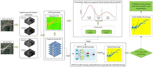
The flow chart of the proposed flood mapping approach is shown in Figure 1. It includes five main steps: (1) spatial–spectral feature extraction from Sentinel-2 MSI images, (2) generation of change magnitude image, (3) uncertainty analysis of change magnitude image, (4) GRNN training and prediction for generating the initial flood map, and (5) two-stage post-processing for generating the final reliable flood map. The details of each step are presented below.

Figure 1. Flow chart of the proposed flood mapping approach.

2.1. Spatial–spectral feature extraction from sentinel-2 MSI images

2.1.1. Spectral indices

Remote sensing images record the spectral reflectance information of various surface objects, which provide a basis for distinguishing various types of surface objects in the image. Several studies have proven that the spectral indices calculated from the original image can better distinguish certain types of surface objects (Goffi et al. 2020; Solovey 2020). Therefore, several spectral indices were selected and calculated to distinguish water bodies and non-water bodies better in the Sentinel-2 MSI image: Normalized Difference Water Index (NDWI) (McFeeters 1996), modified NDWI (MNDWI) (Xu 2006), Normalized Difference Flooding Index (NDFI) (Boschetti et al. 2014), Soil-Adjusted Vegetation Index (SAVI) (Huete 1988), Automated Water Extraction Index (AWEI) (Feyisa et al. 2014), AWEI_SH (Feyisa et al. 2014), and Water Ratio Index (WRI) (Shen and Li 2010). The calculation methods and references of these indices are shown in Table 1.

Table 1. Spectral indices used in this paper.

Spectral indices	Reference
$NDWI={\displaystyle \frac{{\rho }_{Green}-{\rho }_{NIR}}{{\rho }_{Green}+{\rho }_{NIR}}}$	(McFeeters 1996)
$MNDWI={\displaystyle \frac{{\rho }_{Green}-{\rho }_{SWIR1}}{{\rho }_{Green}+{\rho }_{SWIR1}}}$	(Xu 2006)
$NDFI={\displaystyle \frac{{\rho }_{Red}-{\rho }_{SWIR2}}{{\rho }_{Red}+{\rho }_{SWIR2}}}$	(Boschetti et al. 2014)
$SAVI={\displaystyle \frac{(1+L)\ast ({\rho }_{NIR}-{\rho }_{Red})}{{\rho }_{NIR}+{\rho }_{Red}+L}}$	(Huete 1988)
$AWEI=C1\ast ({\rho }_{Green}-{\rho }_{SWIR1})-(C2\ast {\rho }_{NIR}+C3\ast {\rho }_{SWIR2})$	(Feyisa et al. 2014)
$AWE{I}_{SH}={\rho }_{Blue}+D1\ast {\rho }_{Green}-D2\ast ({\rho }_{NIR}+{\rho }_{SWIR1})-D3\ast {\rho }_{SWIR2}$	(Feyisa et al. 2014)
$WRI={\displaystyle \frac{{\rho }_{Green}+{\rho }_{Red}}{{\rho }_{NIR}+{\rho }_{SWIR1}}}$	(Shen and Li 2010)

In Table 1, C1 = 4, C2 = 0.25, C3 = 2.75, D1 = 2.5, D2 = 1.5, D3 = 0.25, and L = 0.5; the Sentinel-2 MSI bands used in this paper are Blue = band2 (490 nm), Green = band3 (560 nm), Red = band4 (665 nm), NIR = band8 (842 nm), SWIR1 = band11 (1610 nm), and SWIR2 = band12 (2190 nm).

2.1.2. Spatial structure feature extraction based on mathematical morphology

Many studies have shown that spatial features (or structural information) can enhance the distinguishability between different surface objects in remote sensing images and improve the accuracy of image classification (Lv et al. 2014; Zhang, Bruzzone, et al. 2018; Zhang, Zhang, et al. 2018; Hao et al. 2020). In recent years, spatial structure features based on mathematical morphology have been widely used in remote sensing image classification or change detection tasks. Therefore, in this paper, spatial features based on mathematical morphology were extracted from Sentinel-2 MSI images to enhance the distinguishability of water bodies from other objects and improve the accuracy and reliability of flood mapping. Specifically, an improved morphological profile (MP) based on multi-shaped Structuring Elements (SEs), which was proposed by Lv et al. (2014), was used. Mathematical morphology uses SEs with known shapes to extract structural information from images. Its basic operations are expansion and erosion. Opening and closing are two important operations based on expansion and erosion. MPs based on multi-shaped SEs are defined based on opening and closing operations. S = {S1, S2, …  … , Sn, n = 1,2,3 … } represents a shape set containing n shapes, and Sn represents the n-th shape with a given size in SE. For the image X, the morphological structure feature MPs containing different shapes of SE can be defined as the combination of image contours generated by the opening and closing operations, as shown in Equation (1(1) $M{P}^{\left(2n+1\right)}\left(X\right)=\left[se{t}_{S_n}^{\left(n\right)}\left(X\right),\dots ,se{t}_{S_1}^{\left(1\right)}\left(X\right),X,{\gamma }_{S_1}^{\left(n\right)}\left(X\right),{\gamma }_{S_n}^{\left(n\right)}\left(X\right)\right],$(1) ), and these structural features are constructed by using SEs with different shapes but the same size. (1) $M{P}^{\left(2n+1\right)}\left(X\right)=\left[se{t}_{S_n}^{\left(n\right)}\left(X\right),\dots ,se{t}_{S_1}^{\left(1\right)}\left(X\right),X,{\gamma }_{S_1}^{\left(n\right)}\left(X\right),{\gamma }_{S_n}^{\left(n\right)}\left(X\right)\right],$(1) where $se{t}_{S_i}$and${\gamma }_{S_i}$respectively represent the result of the closing operation and the opening operation on the image X with the i-th SE, and i = 1,2, … n. For one band of image X, MPs contain n SEs with different shapes, and 2n new features can finally be obtained (excluding the original image band). More details about MPs based on multi-shaped SEs can be traced in (Lv et al. 2014).

In this paper, MPs based on multi-shaped SEs were used on the Red, Green, and Blue bands of Sentinel-2 MSI images to extract their spatial structure features. The shape set used for SE was $S=\{s:s{=}^{\mathrm{\prime }}dis{k}^{\mathrm{\prime }}{,}^{\mathrm{\prime }}lin{e}^{\mathrm{\prime }}{,}^{\mathrm{\prime }}squar{e}^{\mathrm{\prime }}{,}^{\mathrm{\prime }}diamon{d}^{\mathrm{\prime }}\}$ with a fixed size of 4 × 4 pixels. Here, 24 new spatial structure features were extracted.

In this step, all the extracted spectral features, spatial structure features, and six original spectral bands of Sentinel-2 MSI image are stacked to construct feature sets before and after flood events, which will be used as input for the subsequent steps. The stacked feature set is expressed as follows: (2) $F_t=\left[f\right(F_t^{SB});f(F_t^{SI});f(F_t^{Spa}\left)\right],t=1,2$(2) Where $f\left(\cdot \right)$ represents the normalization operation based on Z-score, which is used to eliminate the magnitude difference between different features; $F_1$ and $F_2$ correspond to the feature sets before and after the flood, respectively; $F_t^{SB}$, $F_t^{SI}$, and $F_t^{Spa}$ represent the original spectral bands of the image, spectral index features, and spatial structure features, respectively.

2.2. Generation of change magnitude image

To extract the flooded areas from the bi-temporal Sentinel-2 images, a Change Magnitude Image (CMI) before and after the flood must be constructed based on the extracted image feature sets. The CMI reflects the pixel-by-pixel change degree between the images before and after the flood event, that is, the probability that each pixel in the image belongs to the flooded area.

Here, the difference method is first used to calculate the difference image (DI) of each feature before and after the flood directly according to Equation (3(3) $D{I}_i=\left|F_2^i-F_1^i\right|,i=1,2,\dots ,N,$(3) ). (3) $D{I}_i=\left|F_2^i-F_1^i\right|,i=1,2,\dots ,N,$(3) where $D{I}_i$ represents the DI between the i-th feature of the images before and after the flood; $F_1^i$ and $F_2^i$ represent the i-th feature of $F_1$ and $F_2$, respectively; N represents the total dimension of the extracted feature set F₁ or F₂.

Next, an integrated CMI is generated according to Equation (4(4) $CMI=\sqrt{\sum _{i=1}^{N}D{I}_i^2}$(4) ), which reflects the probability that each pixel belongs to the flooded area. In the CMI, a large value implies a great possibility that the pixel belongs to a flooded area. (4) $CMI=\sqrt{\sum _{i=1}^{N}D{I}_i^2}$(4) The feature-by-feature DI and the integrated CMI generated here will be used in subsequent steps for different purposes.

2.3. Uncertainty analysis of CMI

In this subsection, our goal is to extract reliable training samples from the generated CMI for the subsequent distinction between flooded areas and non-flooded areas. Figure 2 shows a real histogram of magnitude of the CMI. In CMI, a larger value indicates that the corresponding pixel is more likely to belong to the flooded area, and vice versa. However, as shown in Figure 2, there are some pixels with moderate change magnitude in the CMI, and they are between the certain changed region and the certain unchanged region. These pixels have high uncertainty, and determining whether they belong to the flooded area or the non-flooded area is difficult. Therefore, to extract reliable samples of flooded areas and non-flooded areas from the CMI accurately, an uncertainty analysis based on FCM clustering is operated on the CMI to divide all pixels in the CMI into three categories: non-flooded area (certain unchanged category), uncertain area, and flooded area (certain changed category). FCM clustering is one of the most popular fuzzy clustering algorithms (Zhang, Bruzzone, et al. 2018). Unlike traditional hard clustering, which strictly divides each element into a class, FCM clustering regards each cluster as a fuzzy set and determines the clustering relationship through the membership of the elements (Dunn 1973). In FCM clustering, each element can belong to different clusters to different degrees at the same time. The fuzzy characteristic of FCM clustering makes it very suitable for the uncertainty analysis of the CMI.

Figure 2. Uncertainty analysis of change magnitude image.

The uncertainty analysis based on FCM clustering divides all the pixels into three clusters by minimizing the objective function shown in Equation (5(5) $J(X;U,V)=\sum _{i=1}^3\sum _{k=1}^n{\left(u_{ik}\right)}^{\lambda }{\parallel x_k-v_i\parallel }^2,$(5) ), namely, certain non-flood pixels, uncertain pixels, and certain flood pixels. (5) $J(X;U,V)=\sum _{i=1}^3\sum _{k=1}^n{\left(u_{ik}\right)}^{\lambda }{\parallel x_k-v_i\parallel }^2,$(5) where $x_k$ represents the value of the k-th pixel in the CMI, $v_i$ represents the cluster center, $U=\left[u_{ik}\right]$ is the fuzzy membership matrix of the CMI and meets the constraint condition${\sum }_{i=1}^3{u}_{ik}=1$, $1\le k\le n$, $u_{ik}\in [0,1]$, and $\lambda \in [1,\mathrm{\infty })$ is a weighted index. The study in literature (Peng et al. 2019)shows that the clustering result is most accurate when $\lambda =2$. Therefore, $\lambda =2$ in this paper. According to the objective function and constraints, the membership matrix and the clustering center are calculated as follows: (6) $u_{ik}=1/\sum _{j=1}^3{(\frac{\parallel x_k-x_i\parallel }{\parallel x_k-x_j\parallel })}^{2/(\lambda -1)},1\le i\le 3,1\le k\le n$(6) (7) $v_i=\sum _{k=1}^n{u}_{ik}^{\lambda }{x}_k/\sum _{k=1}^n{u}_{ik}^{\lambda },1\le i\le 3$(7) In the FCM clustering algorithm, the clustering centers and membership matrix are iteratively updated according to Equations (6(6) $u_{ik}=1/\sum _{j=1}^3{(\frac{\parallel x_k-x_i\parallel }{\parallel x_k-x_j\parallel })}^{2/(\lambda -1)},1\le i\le 3,1\le k\le n$(6) ) and (7(7) $v_i=\sum _{k=1}^n{u}_{ik}^{\lambda }{x}_k/\sum _{k=1}^n{u}_{ik}^{\lambda },1\le i\le 3$(7) ) until the algorithm ends when $\parallel v_i^{\left(t\right)}-v_i^{(t-1)}\parallel \le ϵ$. $ϵ$ is the threshold; $v_i^{\left(t\right)}$ and $v_i^{(t-1)}$ represent the cluster centers of the t-th and t-1th iterations, respectively.

After completing the fuzzy clustering, the membership degree of each pixel belonging to each cluster can be obtained. Then, according to the principle of maximum membership (that is, each pixel belongs to the class corresponding to its maximum membership), each pixel in the CMI can be initially assigned to a specific class (that is, certain non-flood pixels, uncertain pixels, or certain flood pixels). Next, certain flood pixels and certain non-flood pixels are selected as positive samples and negative samples, and input into the subsequent classification.

2.4. GRNN training and prediction for generating the initial flood map

The GRNN, which was first introduced by Specht (1991), is a widely recognized learning algorithm with strong nonlinear mapping capabilities and learning speed. It is a powerful mathematical tool for dealing with complex nonlinear problems. Moreover, GRNN is a forward propagation network and does not require an iterative training. In this step, GRNN was adopted as the core classifier for flooded area mapping.

Figure 3 shows the GRNN network architecture used in this paper, which consists of four layers: input layer, pattern layer, summation layer, and output layer. In the input layer, k neurons correspond to the k dimensions of the sample features in the data set, that is, the number of neurons in the input layer is equal to the feature dimension of the sample (in this paper, the feature dimension of the sample is 37). The samples in the data set are input to the network through the input layer. Each neuron in the input layer is directly connected to each neuron in the pattern layer. The number of neurons in the pattern layer is consistent with the number of training samples in the data set, and the pattern layer realizes a non-linear transformation of the input data. Each neuron in the pattern layer represents a training pattern. The outputs of the pattern layer measure the distance of the input data from the training patterns and are sent to each neuron of the summation layer. The summation layer has two different types of neurons: one D summation neuron (in red) and multiple S summation neurons (in green). The number of S summation neurons is the same as the number of neurons in the output layer (in this paper, the number of S summation neurons is 1). In the summation layer, the D summation neuron is used to compute the sum of unweighted outputs of the neurons in the pattern layer. The S summation neurons are used to calculate the sum of weighted outputs of the neuron. In the output layer, the number of neurons is the same as the dimension of the sample label (in this paper, it is 1). These neurons receive two different outputs from the summation layer and generate the predicted value of the sample label by calculating the ratio between the output value of S summation neurons and the output value of D summation neuron. For an input sample X whose feature vector is $(x_1,x_2,\dots ,x_k)$, GRNN can generate the predicted value $\hat{Y}$ of the output vector Y corresponding to sample X. Predicted $\hat{Y}$ can be calculated according to Equation (8(8) $\hat{Y}\left(X\right)=\frac{\sum _{i=1}^n{Y}_i\cdot \exp (-d_i^2/2{\delta }^2)}{\sum _{i=1}^n\exp (-d_i^2/2{\delta }^2)}$(8) ): (8) $\hat{Y}\left(X\right)=\frac{\sum _{i=1}^n{Y}_i\cdot \exp (-d_i^2/2{\delta }^2)}{\sum _{i=1}^n\exp (-d_i^2/2{\delta }^2)}$(8) (9) $d_i^2=(X-X_i{)}^T\cdot (X-X_i)$(9) where $X_i$ and $Y_i$ represent the input feature vector and output vector of the i-th sample in the training set, respectively; $d_i$ represents the Euclidean distance between testing sample X and training sample $X_i$; n is the number of training samples; $\delta$ is called the spread parameter, which represents the kernel width of the Gaussian function. Spread parameter $\delta$ is the only unknown parameter in the network and needs optimization.

Figure 3. Architecture of GRNN used for flooded area mapping in this paper.

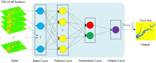
In this paper, the input signal of GRNN is the DI of various features generated in Section 2.2. These features include six original spectral bands, seven spectral index features, and 24 spatial structure features. The output signal is the label of each pixel in the image, indicating whether the pixel belongs to the flooded area. The label of the pixel is 0 or 1, where 0 indicates that the pixel belongs to the non-flooded area, and 1 indicates that the pixel belongs to the flooded area. Therefore, in this paper, the number of neurons in the input layer of the GRNN network is 37, and the number of neurons in the output layer is 1. In addition, the training samples of the GRNN network are reliable samples automatically generated by the uncertainty analysis in Section 2.3 (i.e. certain flood pixels and certain non-flood pixels), and the label rules of these samples are the same as those of the output signal mentioned above. In the samples generated by uncertainty analysis, the difference in the proportion of flood samples and non-flood samples may be evident, and sample imbalance may reduce the accuracy of flood mapping. Therefore, the samples must be properly selected to balance the number of flood samples and non-flood samples. When the number of non-flood samples is substantially greater than that of flood samples, the non-flood samples for the GRNN model training are randomly selected from the samples automatically generated from the uncertainty analysis, and the number of selected non-flood samples is consistent with the number of flood samples. Otherwise, the flood samples are randomly selected from the automatically generated samples to balance the number of flood samples and non-flood samples.

The final flood map generated in this paper is binarized, where 0 corresponds to a non-flooded area, and 1 corresponds to a flood area. However, the original output$\hat{Y}\left(X\right)$ of GRNN calculated according to Equation (8(8) $\hat{Y}\left(X\right)=\frac{\sum _{i=1}^n{Y}_i\cdot \exp (-d_i^2/2{\delta }^2)}{\sum _{i=1}^n\exp (-d_i^2/2{\delta }^2)}$(8) ) is a non-binarized value between 0 and 1. Therefore, the output of GRNN needs to be appropriately modified. After the modification, the final classification label $\hat{Y}(X{)}^{\mathrm{\prime }}$ of each pixel can be expressed as Equation (10(10) $\hat{Y}(X{)}^{\mathrm{\prime }}=⌊\hat{Y}\left(X\right)+\frac{1}{2}⌋,$(10) ). (10) $\hat{Y}(X{)}^{\mathrm{\prime }}=⌊\hat{Y}\left(X\right)+\frac{1}{2}⌋,$(10) Where $\lfloor \cdot \rfloor$ represents the round-down operation. When the original output Y of GRNN is not less than 0.5, the corresponding pixel belongs to the flood area, and $\hat{Y}(X{)}^{\mathrm{\prime }}=1$; otherwise, $\hat{Y}(X{)}^{\mathrm{\prime }}=0$.

In this step, the above GRNN model is trained by 10-fold cross-validation, and the optimal model is selected to generate an initial flood inundation map.

2.5. Two-stage post-processing for generating the final reliable flood map

The initial flooded area map directly generated by the GRNN model inevitably has false detection errors or missed detection errors. For example, several non-flood-induced changed areas or unevident flood-inundation areas may be misclassified. To improve the accuracy and reliability of flood mapping, a two-stage post-processing is proposed to reduce false detection errors and missed detection errors in the initial flood map predicted by GRNN. The proposed two-stage post-processing first eliminates false detection errors as much as possible through the change trend of the water index before and after the flood, and then uses the spatial neighborhood information in the image to enhance the connectivity of the flooded areas to reduce the missed detection errors of flood mapping. After that, a final reliable flood map is generated. The details of this two-stage post-processing are presented as follows.

2.5.1. Stage 1: eliminating false detection errors based on the increase in water index

In Section 2.1, several spectral indices were extracted from the original images. Among them, the MNDWI proposed by Xu (2006) has high sensitivity to water bodies and has been widely used in water-related applications such as water body extraction with remote sensing images (Xu 2006; Singh et al. 2015; Zhai et al. 2015). The change trend of the MNDWI before and after the flood event can reflect the change of the water body. Theoretically, after the flood, the value of MNDWI in the flooded area increases compared with that before the flood. Therefore, in the first stage of post-processing, pixels satisfying Equation (11) are first removed from the initial flooded area, that is, pixels whose MNDWI increase is less than or equal to 0 before and after the flood are excluded from the initial flooded area and marked as non-flood pixels. (11) $MNDW{I}_{post}\text{–}MNDW{I}_{pre}\le 0,$(11) where $MNDW{I}_{pre}$ and $MNDW{I}_{post}$ represent the MNDWI of the images before and after the flood, respectively.

In addition, pixels with MNDWI greater than 0 before the flood are excluded from the flooded area to omit existing water bodies before the flood from the initial flood map (because many existing studies have shown that areas with MNDWI greater than 0 in the image are water bodies).

2.5.2. Stage 2: reducing missed detection errors by enhancing connectivity of the flooded areas

In the flood map after Stage 1 processing, several actual flooded areas may not be extracted effectively, resulting in missed detection errors. Considering the spatial continuity of the flooded area, the spatial neighborhood information of the pixels in the image is used to enhance the connectivity of the flooded area in the flood map in Stage 2, thereby reducing its missed detection errors. Specifically, each pixel in the flood map generated in Stage 1 is first taken as the central pixel, its eight neighborhoods are extracted, and then the number of flood pixels and non-flood pixels in its eight neighborhoods is counted. If the number of flood pixels is greater than or equal to the number of non-flood pixels, then the center pixel is finally determined as a flood pixel; otherwise, it is classified as a non-flood pixel. Several examples of pixels processed by Stage 2 are shown in Figure 4, where green represents flood pixels, and white represents non-flood pixels. A, B, and C are the three processed pixels. Among them, in the previous flood map, flood pixels A and B are misidentified as non-flood pixels, and non-flood pixel C is misidentified as flood pixel. After Stage 2 post-processing, pseudo non-flood pixels A and B are corrected as flood pixels, and pseudo flood pixel C is adjusted to non-flood pixels.

Figure 4. Example of post-processing to enhance the spatial connectivity of flooded areas based on spatial neighborhood information.

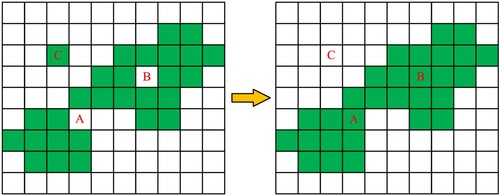
After the spatial connectivity of the flooded areas is enhanced through the above process, the missed detection errors in the flood map can be reduced, and the speckle noise (such as pixel C in Figure 4) in the flood map can also be eliminated to a certain extent to reduce the false detection errors of the flood map further.

After the above two-stage post-processing, the missed detection errors and false detection errors in the initial flooded area map directly generated by the GRNN model are effectively reduced. Finally, a more accurate, reliable flood map can be obtained.

3. Experiments and analysis

3.1. Study area

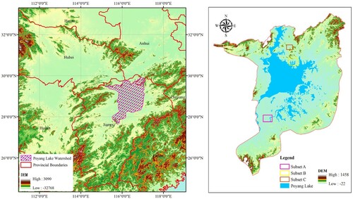
The study area is located in the Poyang Lake Basin in the northern part of Jiangxi Province, China. Poyang Lake is the largest freshwater lake in China, whose area is about 3150 km² at the mean water level. Poyang Lake plays a substantial role in regulating the water level of the Yangtze River in China, conserving water sources, and maintaining the ecological balance of the surrounding area. In the summer of each year, the rainfall in the Poyang Lake area is generally dense and intense, which often causes relatively large floods. Therefore, the study of flood monitoring or inundation area mapping in Poyang Lake area is of great importance and very necessary.

A basin-wide flood broke out in the Poyang Lake area due to continuous heavy rainfall in June and July 2020, causing huge damage and property losses. This paper took this flood event in Poyang Lake area in 2020 as an example, studies how to extract flooded areas accurately and reliably from bi-temporal remote sensing images, and proposes a novel unsupervised approach for automated flooded area mapping from bi-temporal Sentinel-2 MSI images. Three test sites were selected for flood mapping experiments from the entire study area to verify the effectiveness and reliability of the proposed mapping approach. The spatial distribution of these three sites is shown in Figure 5. They contain different types of flooding events and surface conditions with different complexities. The spatial coverage of site A is about 136 km², covering an area where human activities are active, and the surface conditions in this area are the most complicated. The flooded area at site A is mainly due to extreme heavy rainfall and widening of the river bed. The spatial coverage of site B is about 143 km², and its surface conditions are relatively simple, dominated by the water of Poyang Lake, and the flooded area in this area is mainly caused by the skyrocketing water surface of Poyang Lake. The spatial coverage of site C is about 63.5 km², and its surface complexity is between that of sites A and B. The flooded area in this area is mainly due to the dam breach caused by heavy rainfall.

Figure 5. Study area.

3.2.. Experimental data and settings

The data source used in this paper for mapping the flooded areas is composed of multi-temporal Sentinel-2 MSI images downloaded from the official website (https://scihub.copernicus.eu/dhus/#/home) of the European Space Agency (ESA). As shown in Table 2, Sentinel-2 MSI imagery contains 13 spectral bands from VIS/NIR to SWIR with a spatial resolution ranging from 10 meters to 60 meters. The spectral bands used in this paper are Red, Green, Blue, and NIR bands with a resolution of 10 meters, and shortwave SWIR band (SWIR1) and longwave SWIR band (SWIR2) with a resolution of 20 meters. All Sentinel-2 data used have been atmospherically corrected and converted to level 2A products by using the Sen2Cor tool provided by ESA. In addition, the 20-meter resolution SWIR1 and SWIR2 bands were resampled to 10-meter resolution with a special Sentinel-2 resampling tool, which was provided in the SNAP software from ESA. The Sentinel-2 MSI images before and after the flood at the three sites A, B, and C are shown in Figure 6. In addition, the flood reference maps at these three test sites were obtained by visual interpretation.

Figure 6. Experimental images at three test sites.

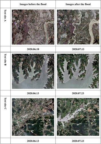
Table 2. Sentinel-2 bands with resolution, central wavelengths and bandwidths.

Band name	Spatial resolution(m)	Central wavelength(nm)	Bandwidth(nm)
B1 Coastal Aerosol	60	443	20
B2 Blue	10	490	65
B3 Green	10	560	35
B4 Red	10	665	30
B5 Red Edge 1	20	705	15
B6 Red Edge 2	20	740	15
B7 Red Edge 3	20	783	20
B8 NIR	10	842	115
B8A NIR Narrow	20	865	20
B9 Water Vapor	60	945	20
B10 Cirus	60	1380	30
B11 SWIR1	20	1610	90
B12 SWIR2	20	2190	180

To test the effectiveness and robustness of the proposed flood mapping approach, experiments were conducted at three selected sites A, B, and C. Three unsupervised change detection methods, namely, CVA_Otsu (Johnson and Kasischke 1998), CVA_FCM (Dunn 1973), and PCA_Kmeans (Celik 2009) were used to map the flooded areas for comparative experiments. In the experiments, the parameters of these methods are mainly determined by trial-and-error method in combination with the parameter settings in some existing studies. Specifically, CVA_Otsu does not require artificially set parameters, and the main parameters that need to be set in the CVA_FCM and PCA_Kmeans methods are the maximum number of iterations and block size, respectively. When the maximum number of iterations in CVA_FCM is small, CVA_FCM may produce unstable results and reduce the mapping accuracy. In this study, trial-and-error method was used to determine that the maximum number of iterations in CVA_FCM was set to 200, and other parameters of CVA_FCM were set to default values. The optimal block size in the PCA_Kmeans method is generally determined according to the spatial resolution of the remote sensing image used. Therefore, the trial-and-error method is used to determine that the block size is set to 6 in this study, and the other parameters remain the default values. In these methods, the influence of these parameters on the mapping accuracy can refer to the existing literature (Dunn 1973; Johnson and Kasischke 1998; Celik 2009). The two-stage post-processing presented in Section 2.5 was also used on the direct change detection results of CVA_Otsu, CVA_FCM, and PCA_Kmeans to generate their corresponding flood mapping results. Moreover, four commonly used accuracy evaluation indicators, namely, overall accuracy (OA), Kappa coefficient (KC), false detection rate (FDR), and missed detection rate (MDR) were used to evaluate and compare the mapping accuracy of different methods quantitatively. The definitions and calculation methods of these indicators can be found in the literature (Tong et al. 2018; Lv et al. 2020).

3.3. Experimental results and analysis at test site A

First, the proposed flood mapping approach was tested at site A. The flooded area at site A is mainly caused by extreme heavy rainfall and widening of the river bed. Figure 7 shows the flood maps generated according to different methods. Compared with the reference map, all methods can identify the main flooded areas, but the false detection error of the CVA_Otsu and PCA_Kmeans methods is more serious than that of the proposed approach and the CVA_FCM method in the western part of the site A area, such as the area marked by the red ellipse in Figure 7.

Figure 7. Flood mapping results of different methods at test site A.

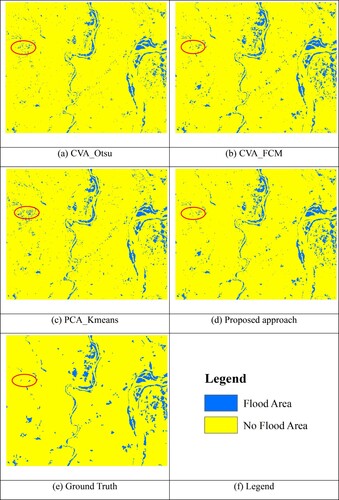
Table 3 shows the mapping accuracy evaluation results of these flood maps by using OA, KC, FDR, and MDR. The OA and KC of the proposed approach are the highest, which shows that the proposed approach has the best overall mapping accuracy among all the methods. CVA_FCM has the second highest overall mapping accuracy, and PCA_Kmeans has the worst mapping performance from the perspective of OA and KC. From the perspective of FDR, the flood map generated by the proposed approach has the lowest FDR, which is approximately 3.43%–12.14% lower than that of other methods. As for MDR, although the MDR of the proposed approach is slightly higher than that of CVA_FCM, it is still lower than that of CVA_Otsu and PCA_Kmeans. Simultaneously reducing FDR and MDR and keeping them at a low level is the key of the proposed approach to achieve good mapping results and superiority over other methods.

Table 3. Accuracy report of flood mapping at test site A.

	CVA_Otsu	CVA_FCM	PCA_Kmeans	Proposed approach
OA	96.9777%	97.8049%	96.5869%	98.0515%
KC	0.7086	0.8133	0.6983	0.8279
FDR	19.39	20.44	28.10	15.96
MDR	34.21	14.33	28.62	16.38

3.4. Experimental results and analysis at test site B

The proposed flood mapping approach was also tested at site B. The flooded area at site B is mainly caused by the surge in the water level of Poyang Lake, which is different from that at site A. Figure 8 shows the results of flood mapping by different methods. The flood maps generated by the proposed approach and the CVA_FCM method are more consistent with the reference map, whereas those produced by the CVA_Otsu and PCA_Kmeans methods have more evident missed detection errors, such as the area marked by the red rectangle in Figure 8. Compared with the proposed approach, several small non-flooded areas are misidentified as flooded areas in several local areas of the flood map generated by CVA_FCM, such as the area marked by the red ellipse in Figure 8. In terms of overall visual effects, the mapping performance of the proposed approach is the best among all methods, followed by CVA_FCM.

Figure 8. Flood mapping results of different methods at test site B.

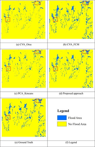
Table 4 shows the result of quantitative accuracy evaluation of flood maps produced by different methods by using OA, KC, FDR, and MDR. The OA and KC of the flood map generated by the proposed approach are the highest among all methods, followed by CVA_FCM, and CVA_Otsu has the lowest OA and KC. The FDR of the proposed approach is remarkably lower than that of other methods, approximately 8.07%–13.32% lower. The MDR of the proposed approach is higher than that of CVA_FCM but remains substantially lower than that of the CVA_Otsu and PCA_Kmeans methods. These quantitative evaluation results prove the effectiveness and reliability of the proposed approach, and show the superiority of the flood mapping performance of the proposed approach.

Table 4. Accuracy report of flood mapping at test site B.

	CVA_Otsu	CVA_FCM	PCA_Kmeans	Proposed approach
OA	94.6960%	97.4465%	94.7029%	98.1034%
KC	0.5290	0.8369	0.5535	0.8646
FDR	15.63	20.25	20.88	7.56
MDR	58.79	8.83	54.27	16.96

3.5. Experimental results and analysis at test site C

A flood mapping experiment at another site C was also conducted to test the effectiveness and robustness of the proposed approach further. Different from test sites A and B, the flooded area at site C is mainly caused by the dam breach. Figure 9 shows the flood maps produced by different methods at site C. Compared with CVA_Otsu and PCA_Kmeans, the flood maps produced by the proposed approach and the CVA_FCM method have better consistency with the reference map. The flood maps produced by CVA_Otsu and PCA_Kmeans clearly show many small areas incorrectly identified as flooded areas, such as the area marked by the red rectangle in Figure 9.

Figure 9. Flood mapping results of different methods at test site C.

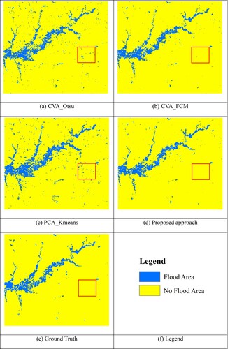
Table 5 shows the results of accuracy evaluation of these flood maps at site C. The OA and KC of the proposed approach are the highest, which indicates that the proposed approach has the best overall mapping performance. The overall mapping performance of CVA_FCM method is second only to the proposed approach. The FDR of the proposed approach is also the lowest among all the methods. The MDR of the proposed approach is slightly higher than that of PCA_Kmeans, but it remains lower than that of CVA_Otsu and CVA_FCM. PCA_Kmeans has the lowest MDR, but its FDR is the highest among all methods because it misclassifies many small areas as flooded areas, which leads to poor overall mapping accuracy. Similarly, the reason for the poor overall mapping performance of the CVA_Otsu method is that its FDR is very high, that is, many actual non-flooded areas are misidentified as flooded areas by the CVA_Otsu method, as shown in Figure 9(a). These quantitative evaluation results show that the proposed approach is effective and has certain advantages in flood mapping performance.

Table 5. Accuracy report of flood mapping at test site C

	CVA_Otsu	CVA_FCM	PCA_Kmeans	Proposed approach
OA	96.8367%	98.7248%	96.1310%	98.8678%
KC	0.7517	0.8903	0.7248	0.9021
FDR	29.80	10.46	37.11	8.87
MDR	15.10	10.11	8.64	9.49

3.6. Analysis of mapping performance of different methods on uncertain pixels

In Section 2.3, all pixels in the image were divided into certain pixels (including certain flood pixels and certain non-flood pixels) and uncertain pixels using the uncertainty analysis of the CMI. As mentioned earlier, these uncertain pixels have a moderate change magnitude between the images before and after the flood; thus, accurately determining whether they are flood pixels or non-flood pixels is often difficult. These uncertain pixels are a major source of errors in flood mapping. Whether these uncertain pixels can be accurately classified can best reflect the performance of a flood mapping method. Therefore, in this subsection, the mapping performances of different methods in dealing with uncertain pixels are further compared and analyzed.

Table 6 shows the OA of different methods on certain pixels and uncertain pixels at all test sites. At the three sites, the classification accuracy of each method on certain pixels is considerably better than that on uncertain pixels, especially at sites B and C, because uncertain pixels are often difficult to classify correctly in flood mapping. Moreover, the OA of the proposed approach on the uncertain pixels is higher than that of other methods at each site to varying degrees. Specifically, the OA of the proposed approach on the uncertain pixels is 0.75%–2.92% higher than that of other methods at site A, 4.19%–21.79% higher than other methods at site B, and 0.77%–9.68% higher than other methods at site C. These results show that compared with the other methods, the proposed approach has certain advantages in correctly classifying uncertain pixels. In addition, Table 6 also shows that the proposed approach not only has better classification accuracy than other methods on uncertain pixels but also on certain pixels, although this accuracy advantage on certain pixels is not as evident as on uncertain pixels. This finding further proves the stability and reliability of the proposed flood mapping approach.

Table 6. OA of different methods on uncertain pixels and certain pixels

	Site A		Site B		Site C
	Uncertain Pixels	Certain Pixels	Uncertain Pixels	Certain Pixels	Uncertain Pixels	Certain Pixels
CVA_Otsu	92.83%	98.73%	68.02%	99.50%	86.40%	99.05%
CVA_FCM	94.77%	99.09%	85.62%	99.58%	94.31%	99.66%
PCA_Kmeans	92.60%	98.27%	69.17%	99.30%	85.40%	98.41%
Proposed approach	95.52%	99.12%	89.81%	99.60%	95.08%	99.67%

4. Conclusions

To map the flooded areas accurately and reliably from Sentinel-2 MSI images, an unsupervised and automated mapping approach based on spatial–spectral features with uncertainty analysis and GRNN is proposed in this paper. First, the spectral and spatial features of the images before and after the flood are effectively extracted, and the CMI is generated. Then, the uncertainty analysis based on FCM clustering is operated on the CMI to generate reliable flood samples and non-flood samples for subsequent flood classification model training. Subsequently, GRNN, a widely used machine learning algorithm with high learning performance, is used to generate the initial flooded area map. Finally, an easy-to-implement two-stage post-processing is constructed and applied to the initial flood map predicted by GRNN to reduce the missed and false detections further, and improve the accuracy and reliability of flood mapping, thereby generating the final reliable flood map. Although the proposed approach uses GRNN as the core classifier, the entire mapping is unsupervised because it uses automatically generated reliable samples for model training instead of a large number of manually labeled samples, which is different from other flood mapping methods based on machine learning. GRNN has a good learning performance and strong nonlinear mapping capabilities. Thus, the proposed mapping approach can better identify the classes of uncertain pixels and improve the accuracy and reliability of flood mapping.

The results of comparative experiments at three selected test areas with different surface conditions in the Poyang Lake Basin prove the effectiveness and superiority of the proposed approach. Compared with the other methods, the proposed approach obtains the best flood mapping accuracy and the lowest false detection rate when the missed detection rate is also maintained at a low level. The proposed approach has clear advantages in correctly classifying uncertain pixels as shown by comparing and analyzing the classification accuracy of different methods on uncertain pixels. In addition, the proposed approach performs well at all three test sites with different surface conditions and different types of floods, which shows the robustness and reliability of the proposed flood mapping approach.

Although optical remote sensing images are not as unaffected by weather conditions and clouds as SAR images, if optical images are available when floods occur, then optical images are undoubtedly still the first choice for flood mapping. At present, the research on flood mapping with optical remote sensing images is relatively lacking. Therefore, the optical image-based flood mapping approach proposed in this paper has certain application potential, especially because the proposed approach is automated and completely unsupervised.

In future research, we will further study how to map the flooded areas quickly, effectively, and reliably from multi-temporal, multi-sensor, and multi-resolution images, especially from the combination of multi-temporal optical and SAR images.

Disclosure statement

No potential conflict of interest was reported by the author(s).

Data availability statement

The Sentinel-2 images used in this study can be downloaded from the official website (https://scihub.copernicus.eu/dhus/#/home) of the European Space Agency.

Additional information

Funding

This work was supported by the National Key Research and Development Program of China under [grant number 2018YFF0215006]; and the Project Supported by the Open Fund of Key Laboratory of Urban Land Resources Monitoring and Simulation, Ministry of Natural Resources under [grant number KF-2019-04-046].

References

- Ahamed, A., and J. D. Bolten. 2017. “A MODIS-Based Automated Flood Monitoring System for Southeast Asia.” International Journal of Applied Earth Observation and Geoinformation 61: 104–117. doi:https://doi.org/10.1016/j.jag.2017.05.006.
- Azareh, Ali, Elham Rafiei Sardooi, Bahram Choubin, Saeed Barkhori, Ali Shahdadi, Jan Adamowski, and Shahaboddin Shamshirband. 2019. “Incorporating Multi-Criteria Decision-Making and Fuzzy-Value Functions for Flood Susceptibility Assessment.” Geocarto International, 1–21. doi:https://doi.org/10.1080/10106049.2019.1695958.
- Berezowski, T., T. Bieliński, and J. Osowicki. 2020. “Flooding Extent Mapping for Synthetic Aperture Radar Time Series Using River Gauge Observations.” Ieee Journal of Selected Topics in Applied Earth Observations and Remote Sensing 13: 2626–2638. doi:https://doi.org/10.1109/JSTARS.2020.2995888.
- Boschetti, M., F. Nutini, G. Manfron, P. A. Brivio, and A. Nelson. 2014. “Comparative Analysis of Normalised Difference Spectral Indices Derived from MODIS for Detecting Surface Water in Flooded Rice Cropping Systems.” PLoS One 9 (2): e88741. doi:https://doi.org/10.1371/journal.pone.0088741.
- Celik, T. 2009. “Unsupervised Change Detection in Satellite Images Using Principal Component Analysis and $k$-Means Clustering.” Ieee Geoscience and Remote Sensing Letters 6 (4): 772–776. doi:https://doi.org/10.1109/LGRS.2009.2025059.
- Choubin, Bahram, Ehsan Moradi, Mohammad Golshan, Jan Adamowski, Farzaneh Sajedi-Hosseini, and Amir Mosavi. 2019. “An Ensemble Prediction of Flood Susceptibility Using Multivariate Discriminant Analysis, Classification and Regression Trees, and Support Vector Machines.” Science of The Total Environment 651: 2087–2096. doi:https://doi.org/10.1016/j.scitotenv.2018.10.064.
- Cian, Fabio, Mattia Marconcini, and Pietro Ceccato. 2018. “Normalized Difference Flood Index for Rapid Flood Mapping: Taking Advantage of EO Big Data.” Remote Sensing of Environment 209: 712–730. doi:https://doi.org/10.1016/j.rse.2018.03.006.
- Dodangeh, Esmaeel, Bahram Choubin, Ahmad Najafi Eigdir, Narjes Nabipour, Mehdi Panahi, Shahaboddin Shamshirband, and Amir Mosavi. 2020. “Integrated Machine Learning Methods with Resampling Algorithms for Flood Susceptibility Prediction.” Science of The Total Environment 705: 135983. doi:https://doi.org/10.1016/j.scitotenv.2019.135983.
- Dunn, J. C. 1973. “A Fuzzy Relative of the ISODATA Process and Its Use in Detecting Compact Well-Separated Clusters.” Journal of Cybernetics 3 (3): 32–57. doi:https://doi.org/10.1080/01969727308546046.
- Feyisa, Gudina L., Henrik Meilby, Rasmus Fensholt, and Simon R. Proud. 2014. “Automated Water Extraction Index: A new Technique for Surface Water Mapping Using Landsat Imagery.” Remote Sensing of Environment 140: 23–35. doi:https://doi.org/10.1016/j.rse.2013.08.029.
- Goffi, Alessia, Daniela Stroppiana, Pietro Alessandro Brivio, Gloria Bordogna, and Mirco Boschetti. 2020. “Towards an Automated Approach to map Flooded Areas from Sentinel-2 MSI Data and Soft Integration of Water Spectral Features.” International Journal of Applied Earth Observation and Geoinformation 84: 101951. doi:https://doi.org/10.1016/j.jag.2019.101951.
- Hao, M., M. Zhou, J. Jin, and W. Shi. 2020. “An Advanced Superpixel-Based Markov Random Field Model for Unsupervised Change Detection.” Ieee Geoscience and Remote Sensing Letters 17 (8): 1401–1405. doi:https://doi.org/10.1109/LGRS.2019.2948660.
- Hosseini, Farzaneh Sajedi, Bahram Choubin, Amir Mosavi, Narjes Nabipour, Shahaboddin Shamshirband, Hamid Darabi, and Ali Torabi Haghighi. 2020. “Flash-flood Hazard Assessment Using Ensembles and Bayesian-Based Machine Learning Models: Application of the Simulated Annealing Feature Selection Method.” Science of The Total Environment 711: 135161. doi:https://doi.org/10.1016/j.scitotenv.2019.135161.
- Huete, A. R. 1988. “A Soil-Adjusted Vegetation Index (SAVI).” Remote Sensing of Environment 25 (3): 295–309. doi:https://doi.org/10.1016/0034-4257(88)90106-X.
- Johnson, R. D., and E. S. Kasischke. 1998. “Change Vector Analysis: A Technique for the Multispectral Monitoring of Land Cover and Condition.” International Journal of Remote Sensing 19 (3): 411–426. doi:https://doi.org/10.1080/014311698216062.
- Li, L., Y. Chen, T. Xu, K. Shi, C. Huang, R. Liu, B. Lu, and L. Meng. 2019. “Enhanced Super-Resolution Mapping of Urban Floods Based on the Fusion of Support Vector Machine and General Regression Neural Network.” Ieee Geoscience and Remote Sensing Letters 16 (8): 1269–1273. doi:https://doi.org/10.1109/LGRS.2019.2894350.
- Li, Yu, Sandro Martinis, Simon Plank, and Ralf Ludwig. 2018. “An Automatic Change Detection Approach for Rapid Flood Mapping in Sentinel-1 SAR Data.” International Journal of Applied Earth Observation and Geoinformation 73: 123–135. doi:https://doi.org/10.1016/j.jag.2018.05.023.
- Lv, Z., T. Liu, C. Shi, and J. A. Benediktsson. 2020. “Local Histogram-Based Analysis for Detecting Land Cover Change Using VHR Remote Sensing Images.” Ieee Geoscience and Remote Sensing Letters, 1–4. doi:https://doi.org/10.1109/LGRS.2020.2998684.
- Lv, Z. Y., P. Zhang, J. A. Benediktsson, and W. Z. Shi. 2014. “Morphological Profiles Based on Differently Shaped Structuring Elements for Classification of Images With Very High Spatial Resolution.” Ieee Journal of Selected Topics in Applied Earth Observations and Remote Sensing 7 (12): 4644–4652. doi:https://doi.org/10.1109/JSTARS.2014.2328618.
- McFeeters, S. K. 1996. “The use of the Normalized Difference Water Index (NDWI) in the Delineation of Open Water Features.” International Journal of Remote Sensing 17 (7): 1425–1432. doi:https://doi.org/10.1080/01431169608948714.
- Mosavi, Amirhosein, Mohammad Golshan, Saeid Janizadeh, Bahram Choubin, Assefa M. Melesse, and Adrienn A. Dineva. 2020. “Ensemble Models of GLM, FDA, MARS, and RF for Flood and Erosion Susceptibility Mapping: A Priority Assessment of sub-Basins.” Geocarto International, 1–20. doi:https://doi.org/10.1080/10106049.2020.1829101.
- Peng, Bo, Zonglin Meng, Qunying Huang, and Caixia Wang. 2019. “Patch Similarity Convolutional Neural Network for Urban Flood Extent Mapping Using Bi-Temporal Satellite Multispectral Imagery.” Remote Sensing 11 (21), doi:https://doi.org/10.3390/rs11212492.
- Sarker, Chandrama, Luis Mejias, Frederic Maire, and Alan Woodley. 2019. “Flood Mapping with Convolutional Neural Networks Using Spatio-Contextual Pixel Information.” Remote Sensing 11 (19), doi:https://doi.org/10.3390/rs11192331.
- Scotti, Vincenzo, Mario Giannini, and Francesco Cioffi. 2020. “Enhanced Flood Mapping Using Synthetic Aperture Radar (SAR) Images, Hydraulic Modelling, and Social Media: A Case Study of Hurricane Harvey (Houston, TX).” Journal of Flood Risk Management 13 (4): e12647. doi:https://doi.org/10.1111/jfr3.12647.
- Shen, L., and C. Li. 2010. “Water Body Extraction from Landsat ETM+ Imagery Using Adaboost Algorithm.” Paper presented at the 2010 18th International Conference on Geoinformatics, 18–20 June 2010.
- Singh, Kanwar Vivek, Raj Setia, Shashikanta Sahoo, Avinash Prasad, and Brijendra Pateriya. 2015. “Evaluation of NDWI and MNDWI for Assessment of Waterlogging by Integrating Digital Elevation Model and Groundwater Level.” Geocarto International 30 (6): 650–661. doi:https://doi.org/10.1080/10106049.2014.965757.
- Solovey, Tatjana. 2020. “Flooded Wetlands Mapping from Sentinel-2 Imagery with Spectral Water Index: A Case Study of Kampinos National Park in Central Poland.” Geological Quarterly 64 (2): 492–505. doi:https://doi.org/10.7306/gq.1509.
- Specht, D. F. 1991. “A General Regression Neural Network.” IEEE Transactions on Neural Networks 2 (6): 568–576. doi:https://doi.org/10.1109/72.97934.
- Tong, Xiaohua, Xin Luo, Shuguang Liu, Huan Xie, Wei Chao, Shuang Liu, Shijie Liu, A. N. Makhinov, A. F. Makhinova, and Yuying Jiang. 2018. “An Approach for Flood Monitoring by the Combined use of Landsat 8 Optical Imagery and COSMO-SkyMed Radar Imagery.” Isprs Journal of Photogrammetry and Remote Sensing 136: 144–153. doi:https://doi.org/10.1016/j.isprsjprs.2017.11.006.
- Uddin, Kabir, Mir A. Matin, and Franz J. Meyer. 2019. “Operational Flood Mapping Using Multi-Temporal Sentinel-1 SAR Images: A Case Study from Bangladesh.” Remote Sensing 11 (13), doi:https://doi.org/10.3390/rs11131581.
- Xu, Hanqiu. 2006. “Modification of Normalised Difference Water Index (NDWI) to Enhance Open Water Features in Remotely Sensed Imagery.” International Journal of Remote Sensing 27 (14): 3025–3033. doi:https://doi.org/10.1080/01431160600589179.
- Zhai, Ke, Xiaoqing Wu, Yuanwei Qin, and Peipei Du. 2015. “Comparison of Surface Water Extraction Performances of Different Classic Water Indices Using OLI and TM Imageries in Different Situations.” Geo-spatial Information Science 18 (1): 32–42. doi:https://doi.org/10.1080/10095020.2015.1017911.
- Zhang, H., L. Bruzzone, W. Shi, M. Hao, and Y. Wang. 2018. “Enhanced Spatially Constrained Remotely Sensed Imagery Classification Using a Fuzzy Local Double Neighborhood Information C-Means Clustering Algorithm.” Ieee Journal of Selected Topics in Applied Earth Observations and Remote Sensing 11 (8): 2896–2910. doi:https://doi.org/10.1109/JSTARS.2018.2846603.
- Zhang, Guangyun, Rongting Zhang, Guoqing Zhou, and Xiuping Jia. 2018. “Hierarchical Spatial Features Learning with Deep CNNs for Very High-Resolution Remote Sensing Image Classification.” International Journal of Remote Sensing 39 (18): 5978–5996. doi:https://doi.org/10.1080/01431161.2018.1506593.