Estimating high-spatial resolution surface daily longwave radiation from the instantaneous Global LAnd Surface Satellite (GLASS) longwave radiation product

ABSTRACT

In this paper, time extension methods, originally designed for clear-sky land surface conditions, are used to estimate high-spatial resolution surface daily longwave (LW) radiation from the instantaneous Global LAnd Surface Satellite (GLASS) longwave radiation product. The performance of four time methods were first tested by using ground based flux measurements that were collected from 141 global sites. Combined with the accuracy of daily LW radiation estimated from the instantaneous GLASS LW radiation, the linear sine interpolation method performs better than the other methods and was employed to estimate the daily LW radiation as follows: The bias/Root Mean Square Error (RMSE) of the linear sine interpolation method were −6.30/15.10 W/m² for the daily longwave upward radiation (LWUP), −1.65/27.63 W/m² for the daily longwave downward radiation (LWDN), and 4.69/26.42 W/m² for the daily net longwave radiation (LWNR). We found that the lengths of the diurnal cycle of LW radiation are longer than the durations between sunrise and sunset and we proposed increasing the day length by 1.5 h. The accuracies of daily LW radiation were improved after adjusting the day length. The bias/RMSE were −4.15/13.74 W/m² for the daily LWUP, −1.3/27.52 W/m² for the daily LWDN, and 2.85/25.91 W/m² for the daily LWNR. We are producing long-term surface daily LW radiation values from the GLASS LW radiation product.

KEYWORDS:

• Surface longwave radiation
• surface longwave net radiation
• GLASS
• time extension method
• surface radiation budget

1. Introduction

Surface longwave (LW) radiation, one of the two components of the surface radiation budget (SRB), consists of surface longwave upward radiation (LWUP), surface longwave downward radiation (LWDN) and surface longwave net radiation (LWNR) (Cheng and Liang 2016; Liang et al. 2019). The surface LW radiation is a fundamental diagnostic parameter of the land surface, atmospheric, and ocean models because of its role in the energy cycle, global climate change and biogeochemical processes (Pinker et al. 2003; Wang et al. 2014).

So far, many efforts have been made to estimate the instantaneous LW radiation, and many algorithms have been constantly proposed and improved. At the local scale, LW radiation can be measured accurately and continuously by ground-based instruments (e.g. pyrometers). However, the ground measurements not only are very expensive (Gui, Liang, and Li 2010) but cannot represent the spatial variability (Carmona, Rivas, and Caselles 2014). In addition, they cannot meet the requirements of many applications due to their limitations of spatiotemporal representativeness (Journée and Bertrand 2010).

Satellite remote sensing is currently the most effective means for obtaining continuous, high spatiotemporal LW radiation measurements. A great number of versatile algorithms have been developed and applied to estimate surface LW radiation at different scales. Two approaches have been used to derive LWUP from the satellite data. The first algorithm is the temperature-emissivity method which estimates the LWUP directly from the land surface temperature (LST) and broadband emissivity (BBE) products (Bisht and Bras 2010; Hu et al. 2019; Wang and Ma 2019; Wang, Ma, and Shi 2019). Many satellites such as the Moderate Resolution Imaging Spectrometer (MODIS), Visible Infrared Imaging Radiometer Suite (VIIRS), and Spinning Enhanced Visible and Infrared Imager (SEVIRI) can provide operational LST products (Wang, Liang, and Meyers 2008; Göttsche et al. 2016; Yu et al. 2018). The Global LAnd Surface Satellite (GLASS) provides long-term, high quality BBE products (Cheng and Liang 2014; Cheng et al. 2016). Additionally, the BBE can be calculated from the narrowband emissivities of MODIS or ASTER. The uncertainties in current LST and BBE products may affect the accuracy of the calculated LWUP (Wang, Liang, and Meyers 2008; Wang and Liang 2009). The other is the hybrid method, which establishes linear or nonlinear empirical relationships between the LWUP and the top of atmosphere (TOA) radiances via extensive radiative transfer simulations (Tang and Li 2008; Cheng and Liang 2016; Zhou and Cheng 2018; Qin et al. 2020). This method may bypass the problem of separating LST and emissivity and achieve more accurate LWUP estimates (Wang and Liang 2009).

Given the screening level air temperature and/or water vapor and cloud parameters, bulk formulae were developed to estimate the LWDN (Brunt 1932; Prata 1996; Crawford and Duchon 1999; Duarte, Dias, and Maggiotto 2006; Carmona, Rivas, and Caselles 2014). Because the input parameters are easy to obtain, the bulk formulae have been widely applied at local and regional scales and their accuracies are acceptable (Cheng, Yang, and Guo 2019; Guo, Cheng, and Liang 2019). However, the coefficients of these bulk formulae are fitted using local measurements and need adjustments when applied to different regions. The hybrid method was developed to accurately estimate clear-sky LWDN (Xu et al. 2016; Cheng et al. 2017). In addition, Zhou et al. (2007) developed the method of estimating clear-sky LWDN from surface self-emissions and column water vapor (CWV) and cloudy-sky LWDN from CWV, surface self-emission and cloud liquid water path. The remaining methods to estimate cloudy-sky LWDN can be grouped into single-layer methods (Forman and Margulis 2007; Wang, Ma, and Shi 2019; Yang and Cheng 2020) and multilayer methods (Gupta, Darnell, and Wilber 1992; Gupta et al. 2010). Clear sky LWDN, cloud-base temperature, cloud fraction and cloud effective emissivity are required in single-layer methods. Because optical sensors cannot penetrate clouds and obtain information for cloud bases, cloud top temperatures (CTT) are always used in the single-layer cloud method. Actually, the cloud base temperature (CBT) dominates the LW radiation from clouds. Thus, Yang and Cheng (Yang and Cheng 2020) constructed a global cloud property database from the collocated MODIS cloud property parameters and cloud vertical structures from the active CloudSat data and then established an empirical relationship for estimating cloud thickness (CT), combined with the reanalysis data, cloud base temperatures were linearly interpolated from cloud top temperatures, cloud top heights and CTs, when the derived CBT was fed into the single-layer cloud method, the accuracy of the cloudy-sky LWDN significantly improved. LWNR is generally calculated by subtracting LWUP from LWDN. All of the methods reviewed above are used for estimating the instantaneous surface LW radiation. Compared with instantaneous LW flux, daily average surface LW radiation or diurnal cycle of surface LW radiation radiation have more application for hydrological, meteorological, agricultural research on global and regional scale (Brooks and Minnis 1984; Lagouarde and Brunet 1993; Bastiaanssen 2000; Allen, Trezza, and Tasumi 2006; Samani et al. 2007).

However, the studies regarding the estimate of daily LW radiation are rarely scarce. Lagouarde and Brunet (1993) first proposed a scheme to estimate daily LWUP obtained from satellite data during under clear-sky, and the daily land surface temperature was calculated using the half-sine function (Lagouarde and Brunet 1993). At present, only the Clouds and the Earth’s Radiant Energy System – Synoptic TOA and surface fluxes and clouds (CERES – SYN) satellite product provides the long-term daily surface LW radiation, but its spatial resolution (1 deg) is coarse (Doelling et al. 2013; Rutan et al. 2015; Doelling et al. 2016). High spatial resolution LW radiation product (down to 1 km) are important diagnostic parameters for mesoscale land surface and weather prediction models, particularly over heterogeneous areas (Christensen et al. 1998; Wenhui, Shunlin, and Augustine 2009). High spatial resolution surface LW radiation product serves as an intermediate scale for the validation of coarse spatial resolution surface LW radiation product. In this context, we have developed a long-term all-sky 1-km instantaneous surface LW radiation product from MODIS data, named as the GLASS LW radiation product (Liang et al. 2021). Some users have put forward the demand for the daily surface LW radiation product. Therefore, we attempted to estimate the daily surface LW radiation product from the instantaneous GLASS LW radiation product. Therefore, it is necessary to develop the method of estimating daily surface LW, and generate the high-spatial resolution surface daily LW radiation products.

Usually, there are two types of methods to calculate daily surface LW radiation, without using sparse satellite observations. The first type is parameterization scheme, which is often employed in the process of estimating the daily average net radiation. Given the daily atmospheric emissivity or daily water vapor pressure at the screen level (Swinbank 1963; Brutsaert 1975), daily air temperature at 2 m, and the land surface emissivity and daily land surface temperature, the surface daily LWDN and LWUP can be calculated, respectively. The daily air temperature and land surface temperature can be obtained by integrating a third-order polynomial or half-sine function on [0, 24] with four observations from polar orbit satellite data (Long, Gao, and Singh 2010; Hou et al. 2014) such as MOD/MYD 07_L2 and MOD/MYD 11_L2. Daily LWNR is obtained from daily LWDN minus daily LWUP. This method is generally applied to calculate the daily LWUP, LWDN and LWNR values under clear-sky conditions and does not need instantaneous LW radiation values (Ortega-Farias, Antonioletti, and Olioso 2000). In addition, daily LWNR can be calculated directly by the FAO-56 Penman method with the maximum and minimum temperature, actual vapor pressure and relative sunshine duration for a clear sky. By incorporating the effect of cloudiness, the Penman method can be used to calculate the cloudy-sky LWNR (Penman 1948; Allen et al. 1998; Irmak, Odhiambo, and Mutiibwa 2011). Another type of method is half-sine interpolation, which uses sine functions to simulate the variations in surface LW radiation whose diurnal variations generally present sinusoidal variations for daylight hours during relatively cloud-free periods. Brooks and Minnis (1984) first proposed the half-sine function and employed it to simulate the diurnal cycle of the Earth Radiation Budget Experiment (ERBE) data and to estimate monthly LW radiation. Young et al. (1998) adopted the half-sine function method to simulate diurnal cycles for the CERES TOA LW radiation under clear and all-sky conditions. In the simulation process, linear interpolation substituted for half-sine modeling in the daytime if the required observations were lacking or if any observed values of the daytime LW radiation were less than the adjacent nocturnal values or if the half-sine function had a negative amplitude.

The use of hourly geostationary (GEO) satellite measurements is an effective way to calculate daily surface LW radiation. The geostationary-data-enhanced temporal interpolation method can address the insufficiently sampled diurnal cycle by incorporating high temporal resolution data from geostationary satellites (GOES) radiation data. Doelling et al. (2013) verified that the geostationary-data-enhanced temporal interpolation method reduced the uncertainty by 20% in the estimated daily TOA LW radiation when compared to CERES-only (CO) half-sine temporal interpolation method using both Terra and Aqua data, or reduce approximately 34% in the estimated daily TOA LW radiation when compared to CO method for Terra or Aqua TOA LW radiation. Afterwards, Rutan et al. (2015) adopted geostationary-data-enhanced temporal interpolation method for the estimate of the daily and monthly mean surface LWDN from CERES SYN1deg. The daily LWDN errors of the SYN1deg was lower or comparative to that of the ISCCP FD and SRB3.0 and MERRA products. Forman and Margulis (2009) presented a climatological lookup table method to estimate the diurnal cycle of LWDN and surface shortwave radiation by combining the data from geostationary and polar-orbiting satellites data, which can reasonably capture temporal variability in the observed fluxes. These studies suggest that increasing the number of observations of LW radiation maybe capture the subtle variations in LW radiation and improve the accuracy of daily LW radiation estimates.

In addition, the concepts or methods used for estimating daily average surface net radiation or shortwave radiation can also be adapted to the estimate of daily LW radiation because they have similar diurnal cycles. These methods can be classified into three major categories: (1) polynomial regression (Olofsson and Eklundh 2007; Xu et al. 2016; Yan et al. 2018), (2) sinusoidal methods (Bisht et al. 2005; Bisht and Bras 2010, 2011; Hwang et al. 2013; Roupioz et al. 2016), and (3) weighted sine methods (Wang et al. 2010; Yan et al. 2018; Zhou et al. 2018).

The Global LAnd Surface Satellite (GLASS) surface LW radiation product includes the instantaneous LWUP, LWDN and LWNR datasets generated from the Terra and Aqua MODIS satellite observation platforms (Zeng, Cheng, and Dong 2020). The GLASS LW radiation product provides at least four observations per day except for orbital gaps and satisfies the requirements of the piecewise linear interpolation, half-sine (linear sine) function, polynomial interpolation, and weighted sine methods. Hence, these four methods were chosen to simulate the daily cycle of LW radiation and estimate the daily average values using GLASS LW radiation product.

This paper is organized as follows: Section 2 describes the site measurements used, the GLASS LW radiation product, and the time extension methods. Section 3 evaluates the performance of time extension methods and provides the estimated results of daily surface LW data from the GLASS LW radiation product. Section 4 discusses ways of improving the accuracy of estimates of daily surface LW radiation. Section 5 concludes this paper.

2. Data and methods

2.1. Ground measurements

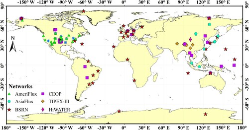
Globally distributed surface radiation flux networks are capable of providing continuous surface LW radiation measurements to support the evaluation of various surface LW radiation products. In this study, we collected ground measurements from 141 sites within six independent flux networks to validate the estimated daily average surface LW radiation. These sites include 10 sites from the Asian network of flux stations (AsiaFlux) (Baldocchi et al. 2001), 30 sites from the AmeriFlux network (Baldocchi et al. 2001), 31 sites from the Baseline Surface Radiation Network (BSRN) (Ohmura et al. 1998), of which 20 are without LWUP measurements; 40 sites from Coordinated Enhanced Observing Period (CEOP), 11 sites from the Third Tibetan Plateau Atmospheric Scientific Experiment (TIPEX-III) (Zhao et al. 2018) and 19 sites from the Multi-Scale Observation Experiment on evapotranspiration over heterogeneous land surfaces in the middle reaches of the Heihe River Basin (HiWATER-MUSOEXE) (Xu et al. 2013; Liu et al. 2016). For detailed site information, please refer to Table A.1. The LWUP and LWDN in BSRN and CEOP were measured by Eppley precision radiometers (PIRs). Their uncertainty estimation is ±6% or 15 W/m², as claimed by the manufacturer at the 95% confidence level (Wang and Dickinson 2013) while the actual uncertainty of PIRs may be much lower than this specification after field calibration (Philipona et al. 1998). Moreover, Kipp & Zonen CG 4 pyrometers were used for measurements of LWUP and LWDN in BSRN and their maximum uncertainty is below 3% for daily totals at the 95% confidence level (http://www.kippzonen.com/?product/17152/CGR+4.aspx). AsiaFlux and AmeriFlux employ Kipp & Zonen net radiometers (e.g. CNR1, CNR4 or CNR1-lite) to measure LWUP and LWDN and their uncertainties for the daily totals do not exceed 10% at the 95% confidence level (Wang and Dickinson 2013). Kipp & Zonen net radiometers (CNR1, CNR4 or CNR1-lite) were also used to measure LW radiation in HiWATER-MUSOEXE and the measurement differences for all CNR1/CNR4 Kipp & Zonen net radiometers were 10 W/m² (daytime) and 5 W/m² (nighttime) (Xu et al. 2013) when compared with an Eppley precision radiometer. Three years of high-quality instantaneous LWUP and LWDN data were extracted from these sites and the daily LWUP and LWDN were derived by averaging these instantaneous values if the instantaneous points for LWUP and LWDN exceeded 80% of the total instantaneous points in a day. The daily LWNR is the difference between daily LWDN and LWUP. Figure 1 shows the geographical distribution of the 141 selected sites. A total of 13 sites are located at high latitudes (60°∼90°), 108 sites are at middle latitudes (30°∼60°), and 20 sites are at low latitudes (0°∼30°). Moreover, these sites cover various land surface types and have different elevations; the details for these sites are listed in Table A.1.

Figure 1. Geographical distribution of the selected ground sites

2.2. GLASS LW radiation product

The GLASS LW radiation product is produced from TERRA-MODIS and AQUA-MODIS observations and has at least four overpass times per day and is freely available to the public (http://www.glass.umd.edu/ and http://www.geodata.cn/thematicView/GLASS.html). The clear-sky LWUP and LWDN values were estimated by the developed hybrid methods (Cheng and Liang 2016; Cheng et al. 2017). The cloudy-sky LWUP was calculated from the land surface temperature provided by MOD06_L2/MYD06_L2 and the GLASS BBE product (Liang et al. 2013; Cheng and Liang 2014; Cheng et al. 2016) whereas the cloudy-sky LWDN was calculated by the single-layer cloud method (Prata 1996; Forman and Margulis 2007). The LWNR was calculated by subtracting LWUP from LWDN. The time span ranged from 2000 to 2020. The spatial resolution of the GLASS LW radiation product is 1 km. The accuracy of clear-sky of the GLASS LW radiation product has been demonstrated to be accurate at global scales (Zeng, Cheng, and Dong 2020) with a bias/RMSE of −4.33/18.15 W/m² for the LWUP, −3.77/26.94 W/m² for the LWDN and 0.70/26.70 W/m² for the LWNR, respectively. The accuracies of the GLASS LW radiation product are higher or comparable to those of other available LW products such as the International Satellite Cloud Climatology Project-Flux Data (ISCCP-FD) (Zhang et al. 2004; Zhang, Rossow, and Stackhouse Jr 2007), Global Energy and Water Cycle Experiment-Surface Radiation Budget (GEWEX-SRB) (Pinker et al. 2003) and Clouds and the Earth’s Radiant Energy System-Gridded Radiative Fluxes and Clouds (CERES-FSW) (Kratz et al. 2020). The GLASS LW radiation product also performs well in climate-change-sensitive areas such as poleward areas, semiarid areas, and the Tibetan Plateau (Zeng, Cheng, and Dong 2020). As stated in the Introduction section, using CTT as a surrogate of CBT in a single-layer method inevitably leads to the LWDN estimation errors (Diak et al. 2000; Forman and Margulis 2009). We are updating the cloudy-sky LWDN algorithm with Yang and Cheng (2020) in the GLASS LW radiation product.

2.3. Descriptions of time extension methods

The employed time extension methods were originally designed for clear-sky land surface conditions. They were applied to cloudy conditions and ocean surface by adding some constraints in this study. The overpass times for the GLASS LW radiation product are consistent with MODIS overpass times which generally have four daily overpass times (two in the daytime and two at night). In this study, we made a constant nightly LW flux assumption (Brooks and Minnis 1984). The daytime LW flux is closely related to the effects of solar heating and its diurnal changes occur as approximately sinusoidal variations (Young et al. 1998) and depend on the sunrise ($t_{sr}$) and sunset ($t_{ss}$) times. Provided with the site coordinates and the date, $t_{sr}$ and $t_{ss}$ can be calculated with the NOAA Sunrise/Sunset and Solar Position Calculators (Meeus 1991), which provides the prepared spreadsheets (NOAA_Solar_Calculations_day.xls and NOAA_Solar_Calculations_year.xls available from https://www.esrl.noaa.gov/gmd/grad/solcalc/calcdetails.html) to calculate $t_{sr}$ and $t_{ss}$ for a day or a year. The detailed equations of $t_{sr}$ and $t_{ss}$ are as follows: (1) $G=(\mathrm{J}\text{-}2451545)/36525$(1) (2) $\mathrm{K}=0.016708634-(0.000042037+0.0000001267\mathrm{G})\mathrm{G}$(2) (3) $\mathrm{R}=23+(26+\left(\right(21.448\text{-}\mathrm{G}(46.815+\mathrm{G}(0.00059\text{-}0.001813\mathrm{G}\left)\right)\left)\right)/60)/60+0.00256\mathrm{c}\mathrm{o}\mathrm{s}\mathrm{d}(125.04\text{-}1934.136\mathrm{G})$(3) (4) $\delta =\arcsin (\sin (R)\sin (P\left)\right)$(4) (5) $ha=\arccos [\frac{\cos \left(90.833\right)}{\cos \left(lat\right)\cos \left(\delta \right)}-\tan \left(lat\right)\tan \left(\delta \right)]$(5) (6) $Snoon=(720-4lon-eqtime+60timezone)/1440$(6) (7) $t_{ss}=(1440Snoon+4ha)/1440$(7) (8) $t_{sr}=(1440Snoon-4ha)/1440$(8)

Here all variables related to the above equations are described according to the contents in the above two spreadsheets:

• $\mathrm{J}$ = Julian date;

• $G$= Julian Century;

• K =  Eccent Earth Orbit;

• $\mathrm{R}$= Ecliptical longitude of the sun (deg);

• $\delta$ = declination of the sun (deg);

• P =  Obliquity of the ecliptic (deg) and $eqtime$ = Equation of time (minutes), please see the above two spreadsheets for their detailed calculations;

• $ha$ =  Hour angle of the sunrise (deg);

• $lat$ =  Latitude (deg);

• $lon$ =  Longitude (deg);

• $timezone$ =  Time Zone, calculated from the longitude;

• $Snoon$ =  Solar noon for a given location (minutes).

Hence, the LW radiation levels at sunrise and sunset were set as constants, and the corresponding LW values were the average LW radiation levels during nighttime. Therefore, there are four LW radiation values in daytime including those from the two GLASS LW overpass times and the sunrise and sunset times that are applied to simulate the diurnal cycles of surface LW radiation.

2.3.1. Piecewise linear interpolation

Piecewise linear interpolation ignores the specific diurnal variations of the surface LW radiation in favor of filling the entire day (Brooks and Minnis 1984). This method applies to irregular scenes. The instantaneous LW value $LW\left(t\right)$ at any time t during the day, can be interpolated as (9) $LW\left(t\right)=\frac{t_2-t}{t_2-t{}_1}LW\left(t_1\right)+\frac{t-t_1}{t_2-t{}_1}LW\left(t_2\right)$(9) where $t$ is the time between $t_1$ and $t_2$, and $t_1$ and $t_2$ are the times between sunrise and sunset, respectively.

2.3.2. The linear sine interpolation

Linear sine interpolation (also called half-sine interpolation) was proposed by Minnis and Harrison (Brooks and Minnis 1984). For a clear day, the general shape of the surface LW radiation curve versus time is always similar in shape: during the daytime, it can be approximated by a portion of a half-sine function whereas during the nighttime, there are no large changes so the curve can be described by a line. Given that the sinusoidal method has been applied to estimate clear- and cloudy-sky surface net radiation (Bisht and Bras 2010) and all-sky top of atmosphere (TOA) LW radiation (Young et al. 1998), this study directly applies the linear sine interpolation method to estimate the all-sky LW radiation. Generally, the daytime surface LW radiation data are fitted by a linear sine function with least-squares fitting while the nighttime data are averaged as a constant value for all nighttime hours. Then, the daily LW radiation is calculated by integrating the fitted LW radiation from 0 to 24 h.

To better implement this method, we imposed several constraints: (1) there must be at least two daytime observation, (2) there must be one or more nighttime observations, (3) all daytime observations must be much greater than the observations during the entire nighttime, and (4) the amplitudes produced by the daytime data must be positive except for the LWNR. If any of the above conditions are not met, piecewise linear interpolation is used. (10) $LW\left(t\right)=a\times sin[\frac{(t-t_{sr})\pi }{t_{ss}-t_{sr}}]+{\overline{LW}}_{night}$(10) where $t_{sr}$ and $t_{ss}$ are the sunrise and sunset times, respectively. ${\overline{LW}}_{night}$ is the average LW value of the nighttime data and a is the amplitude calculated by least-squares fitting.

2.3.3. Piecewise weighted sine interpolation

Piecewise weighted sine interpolation is applicable when there are more than two daytime observations. Based on the sinusoidal curve interpolation method, Wang et al. (2010) developed the weighted sine method to obtain the daily integrated PAR. Afterwards, Yan et al. (2018) used this method to calculate the daily shortwave radiation. Similarly, we used $L{W}_{t_1}\left(t\right)$ to represent the surface LW radiation from sunrise to $t_1$ where $L{W}_{t_n}\left(t\right)$ denotes the LW radiation from $t_n$ to sunset and the LW radiation between $t_1$ and $t_n$ is calculated by piecewise weighted sine interpolation. The criteria for the piecewise weighted sine interpolation are consistent with those for the linear sine interpolation method. To avoid excessive curve simulation caused by the large fluctuations that exist in cloudy-sky LW radiation, the tangent of the slope of the line between two adjacent points during the day was required to be less than 75 degree when simulating the diurnal cycle of GLASS LW radiation; otherwise, piecewise linear interpolation was used. The equation is expressed as follows: (11) $L{W}_{t_i}\left(t\right)-{\overline{LW}}_{night}=(L{W}_{max}-{\overline{LW}}_{night})\sin \left[\right(\frac{t-t_{sr}}{t_{ss}-t_{sr}}\left)\pi \right]$(11) where $L{W}_{max}$ is the maximum value of LW radiation and $L{W}_{max}-{\overline{LW}}_{night}$ is the amplitude. (12) $L{W}_{t_1}\left(t\right)=(L{W}_{t_1}-{\overline{LW}}_{night})(\frac{\sin \left[\right({\displaystyle \frac{t-t_{sr}}{t_{ss}-t_{sr}}\left)\pi \right]}}{\sin \left[\right({\displaystyle \frac{t_1-t_{sr}}{t_{ss}-t_{sr}}\left)\pi \right]}})+{\overline{LW}}_{night}$(12) (13) $L{W}_{t_n}\left(t\right)=(L{W}_{t_n}-{\overline{LW}}_{night})(\frac{\sin \left[\right({\displaystyle \frac{t-t_{sr}}{t_{ss}-t_{sr}}\left)\pi \right]}}{\sin \left[\right({\displaystyle \frac{t_n-t_{sr}}{t_{ss}-t_{sr}}\left)\pi \right]}})+{\overline{LW}}_{night}$(13) where $L{W}_{t_1}$ is the LW value at time $t_1$ and $L{W}_{t_n}$ is the LW value at time $t_n$. Combining functions (11)-(13), the sum of the daily LW radiation in the daytime is expressed as: (14) $L{W}_{\mathrm{d}\mathrm{a}\mathrm{y}time}^{sum}={\int }_{t_{sr}}^{t_1}L{W}_{t_1}\left(t\right)\mathrm{d}t+\sum _i^{n-1}{\int }_{{}_{t_i}}^{t_{i+1}}[\frac{t_{i+1}-t}{t_{i+1}-t_i}L{W}_{t_i}\left(t\right)+\frac{t-t_i}{t_{i+1}-t_i}L{W}_{t_{i+1}}\left(t\right)]\mathrm{d}t+{\int }_{t_n}^{t_{ss}}L{W}_{t_n}\left(t\right)\mathrm{d}t$(14) where the $L{W}_{\mathrm{d}\mathrm{a}\mathrm{y}time}^{sum}$ is the sum of the LW radiation during daytime.

2.3.4. Cubic polynomial interpolation

The curve shape for cubic polynomial fitting is similar to that of a sinusoid. Xu et al. (2016) used quadratic polynomial regression to estimate daily global solar radiation from two instantaneous values. If the total cloud fraction in one day is less than 0.6, the day is regarded as a cloudless day; otherwise, the day is regarded as a cloudy day. Hence, we used cubic polynomial interpolation to estimate the daily LW flux from four instantaneous values under all-sky conditions. Like the linear sine interpolation method, the method was applied for situations when the LW(t) values during the daytime were greater than the average values at night. If the cloudy LW radiation value fluctuated greatly, we calculated the tangent of the slope of the line between two daytime satellite overpass times, the tangent of the line between sunset time and the first daytime satellite overpass time and the tangent of the line between sunset time and the second daytime satellite overpass time. If the absolute value of the first one was larger than the absolute values of the latter two, cubic polynomial interpolation was applied to estimate the daily average LW radiation for the all-sky case. Otherwise, the piecewise linear method was used for interpolating the LW radiation. (15) $LW\left(t\right)=a_1{t}^3+a_2{t}^2+a_{3}t+a_4$(15) where a1, a2, a3 and a4 are coefficients of Equation (15(15) $LW\left(t\right)=a_1{t}^3+a_2{t}^2+a_{3}t+a_4$(15) ).

The daily average LW radiation is expressed as: (16) $L{W}_{average}^{daily}=\frac{{{\int }_0^{t_{sr}}\overline{LW}}_{night}\mathrm{d}t+{\int }_{t_{sr}}^{t_{ss}}LW\left(t\right)\mathrm{d}t+{{\int }_{t_{ss}}^{24}\overline{LW}}_{night}\mathrm{d}t}{24}$(16) where $L{W}_{average}^{daily}$ represents the daily average LW radiation.

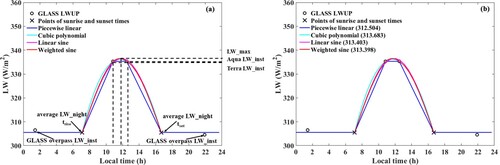
In this study, four different methods were applied to simulate the diurnal cycles of surface LW radiation with the instantaneous GLASS LW radiation data. According to the calculated sunrise and sunset times, we first determined which observations belong to daytime observations and which observations belong to the night observations with the overpass time of GLASS LW radiation product; Then four different methods were used to simulate the diurnal cycles of surface LW radiation with the daytime instantaneous GLASS LW radiation data over the daylight hours, while the night GLASS LW fluxes data was averaged as a constant. Finally, the simulated diurnal variations were used to derive the daily LW radiation by time integration. The schematic for this procedure is shown in Figure 2. Each method produced diurnal LW radiation values at local half-hours, which were integrated to produce the daily values. Figure 2(b) shows an example of the simulated LWUP diurnal cycles with the four time extension methods, as well as the calculated daily LWUP. The simulated LWUP curves are different, but the difference of the calculated LWUPs are small.

Figure 2. (a) Schematic diagram for estimating surface daily LWUP from the GLASS LW radiation with four time extension methods. (b) An example of the simulated LWUP diurnal cycles by using the four time extension methods. The estimated daily LWUP was provided after the name of each time extension method.

3. Results

3.1. Performance of the all-sky instantaneous GLASS LW radiation product

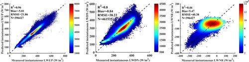
The instantaneous surface LW radiation is a necessary parameter for estimating the daily averaged surface LW radiation. Usually, the instantaneous LW radiation is retrieved and evaluated prior to estimating the daily LW radiation (Bisht et al. 2005; Bisht and Bras 2010; Dongdong et al. 2015; Xu et al. 2016). We first validated the all-sky GLASS LW radiation. According to the cloud mask flag in MOD35_L2/MYD35_L2, we labeled a pixel as clear sky if this pixel was confidently clear-sky or possibly clear-sky whereas a pixel was labeled as cloudy sky if this pixel was cloudy-sky or of an uncertain condition in the GLASS LW radiation product. The temporal matching criterion was determined by the temporal resolution of the site measurement; for example, the time difference between the site observation time and satellite overpass time in one day was less than 15 min if the temporal resolution of the site measurements was 30 min. Figure 3 shows the validation results of GLASS LW radiation under all-sky conditions. The bias, RMSE and R² were −5.81, 21.86 W/m² and 0.96 for the LWUP, respectively; −0.84 and 38.22 W/m² and 0.8 for the LWDN, respectively; and the values were 5.47, 40.38 W/m² and 0.46 for the LWNR, respectively. This accuracy is worse than the validation results of Zeng, Cheng, and Dong (2020) which correspond to the accuracy for confident clear-sky conditions. Because clouds cause the greatest uncertainty in surface LW radiation estimates (Wild et al. 2001; Trenberth, Fasullo, and Kiehl 2009), the accuracy of cloudy-sky surface LW radiation is usually worse than that for clear-sky conditions. Furthermore, the cloud mask flag of probable clear and uncertain conditions also adds additional uncertainties to the validation results in Figure 3.

Figure 3. Validation results for GLASS LW radiation under all-sky conditions.

3.2. Time extension methods applied to ground site fluxes

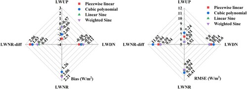
Four time extension methods were first applied to the ground observations to test the feasibility and accuracy of estimating the daily average surface LW radiation. The ground observations were acquired by matching the overpass times of the GLASS LW radiation product. The sunrise and sunset times were calculated by using the latitude and solar declination based on the day of year. Daily LW values were derived by integrating the interpolated values from 0 to 24 h. The validation results for the daily LWUP, LWDN, and LWNR are shown in Figure 4. We also calculated the daily LWNR by subtracting the daily LWUP from daily LWDN and designated it as LWNR-diff. LWNR-diff is also shown in Figure 4 for comparison. We found that the fitting results were much better when the samples were closely distributed along the 1:1 line. The detailed bias, RMSE and R² values are shown by radar maps (Figure 5) There were no significant differences in RMSEs but significant differences were present in the biases. The RMSEs were less than 7.24, 10.6, 10.41 and 11.02 W/m² for the daily LWUP, LWDN, LWNR, and LWNR-diff, respectively; the biases were negative for the LWUP and LWDN while they were positive for the LWNR and LWNR-diff, and the absolute values were less than 2.9 W/m². Among the four time extension methods, the linear sine method performed best for the daily LWUP, LWDN and LWNR-diff with bias/RMSE values of −0.57/5.49 W/m², −0.04/9.85 W/m², 2.06/9.94 W/m² and 0.41/9.59 W/m² respectively, followed by the weighted sine method, the bias/RMSE were −0.66/5.52 W/m², 0.12/9.8, 2.21/9.84 W/m² and 0.66/9.54 W/m². The bias of the cubic polynomial method was less than that of the piecewise linear interpolation method, whereas the RMSE of the former was larger that that of the latter. The piecewise linear interpolation method performed the worst. Given the accurate ground measurements at overpass times for GLASS LW radiation, all time extension methods achieved accurate daily LW radiation estimates, especially the linear sine method.

Figure 4. Comparisons of measured and estimated daily LWUP (first row), LWDN (second row), LWNR (third row), and LWNR-diff (fourth row) by using four time extension methods: piecewise linear interpolation, linear sine interpolation, piecewise weighted sine interpolation, and cubic polynomial interpolation, respectively; sorted by column from left to right.

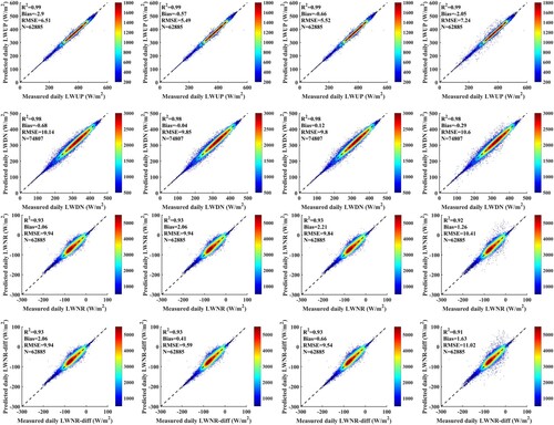
Figure 5. Statistical results of four time extension methods.

3.3. Time extension methods applied to GLASS LW radiation product

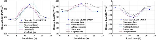
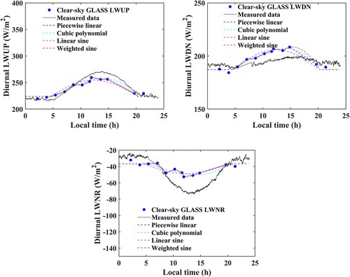
The performances of the four time extension methods were evaluated in this section by the GLASS LW product. The LW radiation values at sunrise and sunset are the average of the night points in a day. The instantaneous GLASS LW radiation values in the day were chosen to simulate the diurnal cycle. Figure 6 shows comparisons between ground-measured LW radiation and simulated LW radiation by the four time extension methods with the GLASS LW product. Clearly, all methods only approximately described the diurnal variations but failed to adequately capture the fluctuations in all-sky LW radiation. These results also reflect the difficulty of estimating daily LW radiation when using only a few points, especially for cloudy-sky conditions. The fluctuations of cloudy-sky LW radiation were much larger than those for clear-sky LW radiation.

Figure 6. Comparisons of the measured and simulated diurnal cycles of clear-sky LWUP, LWDN and LWNR at station ‘SGP E1 Larned’ for DOY 178, 2006.

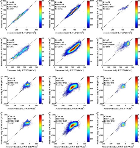
Figure 7 shows the performance of the four time extension methods for estimating daily LW radiation using the GLASS LW product. The daily LWUP was underestimated with biases ranging from −8.59 W/m² to −6.30 W/m² and the RMSEs were less than 16.27 W/m². The biases in the daily LWDN were −2.39, −2.02, −1.65 and −1.43 W/m², respectively and the RMSEs were less than 27.96 W/m² for piecewise linear interpolation, cubic polynomial interpolation, linear sine interpolation, and piecewise weighted sine interpolation methods, respectively. The daily LWNR were overestimated by the four time extension methods with biases ranging from 5.57–6.31 W/m² and the RMSEs were approximately 27 W/m². The accuracy of the estimated LWNR-diff was similar to that of the LWNR.

Figure 7. Performances of four time extension methods for estimating daily LW radiation from the GLASS LW radiation product. Method1, Method2, Method3 and Method4 are the piecewise linear interpolation, cubic polynomial interpolation, linear sine interpolation, and piecewise weighted sine interpolation methods, respectively.

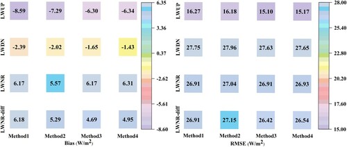
The linear sine interpolation method performed best for estimating daily LWUP with a bias and RMSE of −6.30 and 15.10 W/m², respectively, followed by the weighted sine method whose bias/RMSE −6.34/15.17 W/m²; The linear sine and weighted sine methods performed better than the cubic polynomial and piecewise linear interpolation method in estimating daily LWDN. For the daily LWNR, the accuracy of the four interpolation methods were comparable but the cubic polynomial interpolation had the lowest bias. For the daily LWNR-diff, the linear sine method performed best with a bias and RMSE of 4.69 and 26.42 W/m², respectively. In general, the performances of the four time extension methods did not differ greatly. The sinusoidal methods were slightly better than the other methods, especially the linear sine method, which were consistent with the evaluation results obtained by using ground measurements. For the linear sine method, the bias/RMSE were −6.30/15.10 W/m² for the daily LWUP, −1.65/27.63 W/m² for daily LWDN, 6.17/26.91 W/m² for daily LWNR and 4.69/26.42 W/m² for daily LWNR-diff.

Figure 8 shows the fitted diurnal cycles of LW radiation using GLASS LW radiation product at station ‘SGP E1 Larned’ in June 2006. In this month, the mean and standard deviation values were approximate 440 and 40 W/m² for daily LWUP, 366 and 31 W/m² for daily LWDN, −77 and 30 W/m² for daily LWNR, respectively.

Figure 8. Time series of GLASS LW flux data and the fitted diurnal cycles in daytime at station ‘SGP E1 Larned’ for June 2006. The doy of year (DOY) also represents the local time 12 h each day. (a) represents the diunrnal represents the diunrnal LWUP, (b) represents the diunrnal LWDN, (c) represents the diunrnal LWNR.

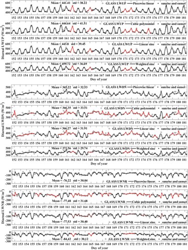
The piecewise linear interpolation method can simulate the diurnal cycle of all-sky LWUP. The remained three methods were failed if there was only one observations in daytime. As shown in Figure 8(a), the piecewise linear interpolation method successfully simulated the diurnal of DOY 162, 165, 171 and 172, but the remained three method failed. In addition, the cubic polynomial interpolation method cannot simulate the diurnal cycle of cloudy LW radiation like DOY 173 and 175, which fluctuated greatly and result the distortion of the diurnal curve.

Regarding the LWDN, the cubic polynomial and linear sine interpolation methods cannot simulate the diurnal cycles of almost half the days, compared with performance of the piecewise linear and piecewise weighted sine interpolation methods. The fitting results are shown in Figure 8(b). The reasons for the poor performance of the cubic polynomial interpolation method was similar to the simulation of the LWUP diurnal cycles. In addition to at least one daytime observation, there are four constraints in the linear sine interpolation method, hence, the piecewise linear interpolation method was used to simulate the diurnal cycles of days such as DOY 166 and 172, instead of the linear sine interpolation method. The performances of the four time extension methods in simulating the diurnal cycles of LWNR were similar to those of LWDN, as we can see by comparing Figure 8(b) and (c). Overall, it is more difficult to simulate the diurnal cycles of LWDN and LWNR than to simulate the diurnal cycles of LWUP.

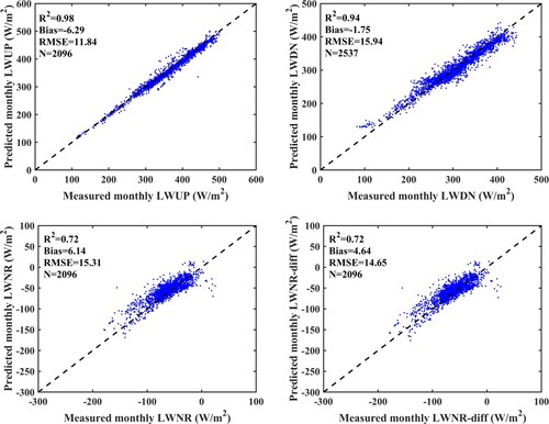
Figure 9 shows the accuracy of monthly LW radiation, which was averaged from the surface daily LW radiation estimated by the linear sine interpolation method. The monthly LWUP showed a bias of −6.29 W/m² and RMSE of 11.84 W/m²; the bias/RMSE of the monthly LWDN were −1.75/15.94 W/m², respectively; the bias/RMSE of the monthly LWNR were 6.14/15.31 W/m², respectively; and the bias/RMSE of the monthly LWNR-diff were 4.64/14.65 W/m², respectively.

Figure 9. The accuracy of the estimated surface monthly LW radiation

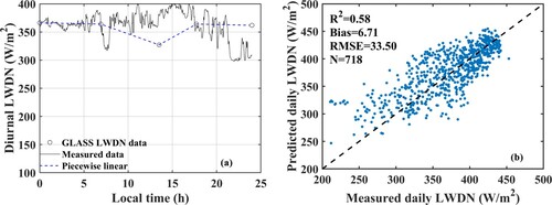
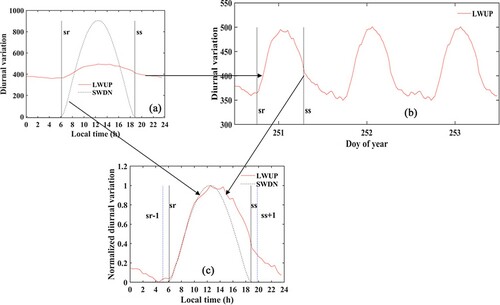
As pointed by Young et al. (1998), there is little diurnal variability in LW flux due to solar insolation over the oceans, and the variations and types of cloud cover over the ocean surface can cause the greatest variations in LW radiation and such variations in LW radiation were assumed to be linear at the ocean surface in their study. We investigate the accuracy of surface LW radiation estimates over the ocean surface separately here. Figure 10 displays the diurnal variations and regular characteristics in the LWDN at site ‘BER’ in DOY 46, 2009. For the small diurnal variation in the LWDN, piecewise linear interpolation was used to simulate the diurnal variation and calculate daily LW radiation values. The estimated accuracies for all four ocean sites are also shown in Figure 10. The R², bias and RMSE were 0.58, 6.71 and 33.50 W/m² for the daily LWDN, respectively. Compared to the overall accuracy of LWDN estimates (Figure 7), the accuracy over the ocean surface was slightly degraded. The first reason was that the solar insolation caused diurnal cycle over the oceans was weak, and the greatest variability in LW fluxes over the oceans occurred due to changes in the amount and types of clouds (Young et al. 1998), which was stated in the beginning of this paragraph. The second was that four times observations from MODIS Terra and Aqua cannot capture the diurnal variability of clouds as well as the caused variations in LW radiation. There are no results for the daily LWUP and LWNR because the corresponding ground measurements were unavailable.

Figure 10. (a) The diurnal cycle of LWDN at ocean station ‘BER’ located near the island of Bermuda in DOY 46, 2009 and (b) the average accuracy of the estimated daily LWDN over ocean sites.

The nighttime LW radiation was assumed as a constant in the time extension methods. The site-measured surface LW radiation were used to investigate the influence of constant LW radiation assumption during nighttime. The constant LW radiation during nighttime were replaced by the site measurements, and GLASS radiation product were used for daytime. The line sine interpolation method was used to calculate the daily surface LW radiation, which was then taken as the reference. The relative errors are less than ±5% for daily LWUP, LWDN, LWNR and LWNR-diff.

3.4. Performance of temporal extension methods at different latitudes

The overpass times of the GLASS LW product were consistent with those of the MODIS products used. A satellite in polar orbit passes over the polar regions and the areas of overlap at high latitudes are more frequent than for middle and low latitudes when the Terra and Aqua satellites operate simultaneously while the earth rotates. Therefore, the GLASS instantaneous LW radiation product has more than four overpass times per pixel in the high-latitude regions which are as high as 14 times (Doelling et al. 2013) each day while the overpass times at middle and low latitudes generally occur four times each day. Greater numbers of instantaneous LW radiation observations make it easier to capture the polar diurnal variability (Zhou et al. 2018) and may be useful for improving the accuracy of daily LW radiation estimates. Figure 11 shows comparisons between the simulated diurnal changes from the four time extension methods and the GLASS LW radiation poleward of 60° latitude. Compared with Figure 6, the polar diurnal variabilities of the LWUP and LWDN were not obvious and the instantaneous absolute values of LW radiation were nearly all lower than those at the middle latitudes.

Figure 11. Site measured and simulated diurnal cycles of the clear-sky LWUP, LWDN and LWNR at station ‘TIK’ on DOY 105, 2016.

The performances of the four time extension methods at three subregions according to their latitudes, i.e. low-latitude region (0°∼30°N, 0°∼30°S), mid-latitude region (30°∼60°N, 30°∼60°S), and high-latitude region (60°∼90°N, 60°∼90°S) are shown in Figure 12. For the daily LWUP, R² decreased as the latitude decreased. The absolute values of the bias were smallest in the low-latitude regions and the daily LWUP was a little underestimated in middle latitude, but it owned the low RMSE in high and middle latitude regions. In high-latitude regions, the linear sine interpolation method performed best with a bias/RMSE of −4.76/13.31 W/m² which was followed by piecewise linear interpolation and weighted sine methods. In mid-latitude regions, the linear sine interpolation and weighted sine interpolation methods were more accurate than the two other methods. The bias/RMSE were approximately −6.3/15.3 W/m². In low-latitude regions, the best method was linear sine interpolation with a bias/RMSE of −1.90/23.57 W/m².

Figure 12. Accuracies of the daily LWUP, LWDN, LWNR and LWNR-diff estimates at low-latitude, mid-latitude, and high-latitude regions. Method1, Method2, Method3 and Method4 denote the piecewise linear interpolation, cubic polynomial interpolation, linear sine interpolation, and piecewise weighted sine interpolation methods, respectively.

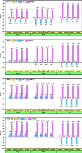
For the daily LWDN, the change of R² was similar to that of the daily LWUP. The daily LWDN values were slightly underestimated in low-latitude regions. In high-latitude regions, the linear sine interpolation method performed best with a bias/RMSE of 2.47/25.03 W/m²_. In mid-latitude regions, the linear sine interpolation method was more accurate than the other three methods. The bias/RMSE were −1.43/27.46 W/m², followed by the cubic polynomial method with the bias/RMSE of −1.63/27.45 W/m². But the diurnal curve that was simulated by the cubic polynomial method showed some differences (to a certain extent) when compared with the other three methods (Figure 6), we prefer the linear sine method. In low-latitude regions, the performances of the four methods were not good. However, the linear sine and weighted sine interpolation method still performed better than the others.

In the daily LWNR estimates, the R² values were quite low in high and low latitude regions. The direct reason was that the instantaneous GLASS LWNR was underestimated, whose bias and RMSE are −13.79 W/m² and an RMSE of 38.85 W/m², respectively. The other one was that the cloud diurnal variations were strong over continental convective regions and over regions of maritime subtropical subsidence (Minnis and Harrison 1984). Four times observations of GLASS LW radiation product cannot capture the cloud variations during the whole day, which will inevitably cause errors in the estimated daily LWNR values. There were no obvious differences for calculating the daily LWNR using four interpolation methods in three regions. The daily LWNR values were seriously underestimated in low-latitude regions. The bias/RMSE were close to 7.8/24.5 W/m² in the high-latitude, 6.5/27.23 W/m² in mid-latitude regions and −11.68/25.5 W/m² in low latitudes, respectively. The differences between the daily LWNR and LWNR-diff were quite small except that the accuracy of the daily LWNR-diff was slightly better in the middle-latitude regions and the corresponding time extension method was linear sine interpolation.

Due to the inconspicuous diurnal variations of LW radiation at high latitudes, the differences in accuracy of the four time extension methods were not significant. Underestimations or overestimations of the daily LW radiation were closely related to the performance of the instantaneous GLASS LW radiation. By examining the evaluation results of the time extension methods, we found that the linear sine interpolation method was more stable than the other methods at different latitudes. Figure 13 shows comparisons between the estimated daily LWUP, LWDN, LWNR and LWNR-diff by the linear sine interpolation method and ground measurements. Due to the greater disparity in sample numbers, the mid-latitude accuracies were similar to those derived from the global samples (Section 3.3). The evaluation results in high-latitude and low-latitude regions may lack representativeness due to the scarcity of samples. The efficacy of the increment in overpass times in high-latitude regions is not significant.

Figure 13. Comparisons between the estimated daily LWUP, LWDN, LWNR and LWNR-diff from the linear sine method and from ground measurements. The columns (from left to right) are the results for the low-latitude, mid-latitude, and high-latitude regions.

3.5. Performance of the daily LW radiation estimate under different scenarios

The diurnal variations of LW radiation are quite pronounced in deserts and tropical wet and dry regions, where the land afternoon convection is prevalent. Hence, we evaluated the performances of four time extension methods in coastal, deserts, tropical wet and dry regions. The accuracy of the four time extension methods are provided in Table 1. Over the desert regions, there is obvious diurnal variability in LW fluxes due to solar heating. The diurnal variability of LW flux generally exhibits a sinusoidal variation in relatively cloud-free periods at the daytime (Minnis and Harrison 1984). Due to limited ground sites, there were only two sites (GOB and AWS19) located in the desert regions. The daily LWUP was seriously underestimated by all the four time extension methods. The absolute bias of daily LWUP were all larger than 15 W/m², and RMSEs were less than 27.72 W/m². For daily LWDN, the bias were less than 3.32 W/m² while RMSEs were more than 30 W/m². The reason for this poor performance may be that the maximum value of the amplitude of LWUP diurnal variation cannot be captured by four satellite observations. The amplitude of LWDN diurnal variation is weaker than that of LWUP, and the errors of four time extension methods in estimating daily LWDN was small than that in estimating LWUP. It finally led to the large overestimation in the daily LWNR-diff, whose bias is large than 14 W/m².

Table 1. The accuracy of the surface daily LW radiation estimate under different surface types.

Region	Method	LWUP		LWDN		LWNR		LWNR-diff
		Bias (W/m^2)	RMSE (W/m^2)	Bias (W/m^2)	RMSE (W/m^2)	Bias (W/m^2)	RMSE (W/m^2)	Bias (W/m^2)	RMSE (W/m^2)
Coastal	Piecewise linear	−7.12	19.17	−6.39	32.89	−0.31	26.72	−0.29	26.72
	Linear sine	−6.12	18.6	−6.14	32.77	−0.31	26.72	−1.01	26.62
	weighted sine	−6.09	18.61	−5.92	32.73	−0.17	26.73	−0.81	26.65
	polynomial	−6.25	19.53	−6.41	33.05	−0.83	27.15	−1.11	27.44
Desert	Piecewise linear	−21.03	27.72	−3.32	31.13	17.69	32.31	17.71	32.32
	Linear sine	−15.28	23.35	−1.72	30.61	17.69	32.31	13.56	30.41
	weighted sine	−16.34	24.11	−1.6	30.94	17.75	32.38	14.74	30.9
	polynomial	−19.31	26.59	−2.28	30.41	16.81	32.18	17.03	31.53
tropical wet and dry regions	Piecewise linear	−15.38	18.19	−16.82	29.1	−10.48	25.32	−10.46	25.32
	Linear sine	−14.06	17.02	−16.21	28.82	−10.48	25.32	−11.4	25.42
	weighted sine	−14.08	17.05	−16.11	28.77	−10.37	25.3	−11.17	25.42
	polynomial	−14.13	17.32	−16.62	29.14	−11.13	25.86	−11.57	25.86

In the coastal regions and tropical wet and dry regions, the accuracy of the daily LW fluxes was also poor. The absolute values of bias were large than 10 W/m² for daily LW radiation. The marine and coastal sites were appeared in these regions (Figure 1), and the accuracy for daily LW radiation estimate over oceans were inherently poor, the reason was discussed in Section 3.3. The coastal sites may be simultaneously affected by the ocean and land convections, the diurnal cycle of cloud radiation forcing was neglected (Loeb et al. 2009), such changes were complicated and even hard to characterize by four times observations of GLASS LW radiation product.

We also evaluated the accuracy of the daily LW radiation estimate in mid-latitude summer and winter. As shown in Table 2, four time extension methods performed better in mid-latitude summer than that in mid-latitude winner. RMSEs were less than 26 W/m² in mid-latitude summer while the values were large than 30 W/m² for daily LWDN and LWNR (LWNR-diff) in the mid-latitude winter. The daily LWUP was obviously underestimated while LWNR was seriously overestimated. The absolute values of bias were generally large than 10 W/m². The potential reason may be that there is a strong land diurnal heating in summer while the cloud conditions are frontal driven in winner, the diurnal cycle of cloud properties impacts the diurnal cycle of LW fluxes.

Table 2. The accuracy of the surface daily LW radiation estimate in mid-latitude summer and mid-latitude winter.

Season	Method	LWUP		LWDN		LWNR		LWNR-diff
		Bias (W/m2)	RMSE (W/m2)	Bias (W/m2)	RMSE (W/m2)	Bias (W/m2)	RMSE (W/m2)	Bias (W/m2)	RMSE (W/m2)
mid-latitude summer	Piecewise linear	−8.88	16.43	−5.12	25.07	3.71	23.34	3.72	23.34
	Linear sine	−5.16	15.11	−3.74	25.01	3.71	23.34	1.46	22.77
	Weighted sine	−5.22	15.1	−3.46	25.05	3.84	23.33	1.79	22.86
	Cubic polynomial	−6.81	16.39	−4.36	25.37	2.88	23.6	2.45	23.7
mid-latitude winter	Piecewise linear	−7.21	18.18	2.88	32.24	10.73	33.19	10.75	33.19
	Linear sine	−6.03	17.59	3.26	32.19	10.73	33.19	9.97	32.73
	weighted sine	−6.07	17.61	3.36	32.18	10.85	33.21	10.10	32.78
	Cubic polynomial	−6.44	17.87	3	32.19	10.37	33.02	10.06	32.9

4. Discussion

4.1. Improving the accuracy of daily LW radiation estimates

Instantaneous LW radiation is the basis for calculating the daily LW radiation. Thus, the accuracy of the instantaneous LW radiation constrains the accuracy of the estimated daily values. This study first estimated the daily LW radiation from the instantaneous ground measurements that were collocated with overpass times for the GLASS LW radiation. The R² values were close to 1, bias values were all almost less than 1.0 W/m² and RMSEs were less than or close to 10 W/m² which indicate that these methods can be applied to calculate the all-sky daily LW radiation. However, large discrepancies appeared when these methods were applied to the GLASS LW product. The biases were from −8.59 to −6.30 W/m² and the RMSEs varied from 16.10–16.27 W/m² for the daily LWUP; the biases ranged from −2.39 to −1.43 W/m² and the RMSEs varied from 27.63–27.96 W/m² for the daily LWDN; the daily LWNR had biases from 5.57–6.31 W/m² and the RMSEs were approximately 26.93 W/m². As we can see in Figure 14, the accuracy of GLASS LW radiation affects the simulated diurnal cycle of LW radiation and therefore the estimated daily values. In short, degradation of the GLASS LW radiation results in degradation of the estimated daily LW radiation. Adjusting the instantaneous LW radiation may be helpful for improving the accuracy of daily LW radiation estimates (Bisht et al. 2005).

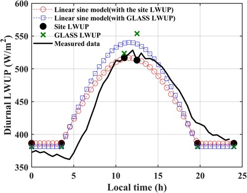
Figure 14. Diurnal cycle of LWUP simulated by linear sine interpolation method with site measurements and GLASS LWUP at high latitude.

Using the collocated GLASS and site LW radiation data, we first fitted the linear relationships for all-sky conditions. The fitting results are shown in Table 3. The instantaneous GLASS LW radiation values were adjusted by the fitted equations. The daily LW radiation was recalculated by using the linear sine interpolation method. The bias, RMSE and R² were −7.39, 9.85 W/m² and 0.99 for the daily LWUP, respectively; −4.1, 16.06 W/m² and 0.98 for daily LWDN, respectively; 7.53, 17.84 W/m² and 0.92 for daily LWNR, respectively; and 4.23, 14.13 W/m² and 0.86 for daily LWNR-diff, respectively. Compared with the results in Figure 7, the RMSEs were clearly lower, but the absolute bias values were slightly higher than those without adjustments except for daily LWDN. Another alternative method is to directly remove the bias from the GLASS LW radiation and then retrieve the daily LW radiation. The biases came from the validation results in Section 3.1. The accuracies of the daily LW radiation values are shown in Figure 15. The bias, RMSE and R² were −0.31, 12.97 W/m² and 0.97 for the daily LWUP, respectively; −0.96, 27.75 W/m² and 0.83 for daily LWDN, respectively; 0.3, 26.17 W/m² and 0.49 for daily LWNR, respectively; and −0.51, 25.97 W/m² and 0.63, respectively for daily LWNR-diff. The biases were significantly reduced, and the RMSEs were a little reduced except the daily LWDN, when compared to the accuracies for those without adjustments (Figure 7). Both methods cannot fully improve the accuracy of the estimated surface daily LW radiation. There are primarily two reasons, one is that the diurnal variations of LWUP, LWDN and LWNR are different, the other is that sparse temporal retrievals cannot capture the diurnal variations of surface LW radiation components.

Figure 15. Accuracies of daily LW radiation estimated from the bias-removed GLASS LW radiation by using the linear sine interpolation method

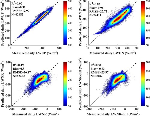
Table 3. The fitted linear functions using GLASS and all fluxnet sites LW radiation data.

Parameter	Fitted equations
LWUP	$\mathrm{y}=1.0054\mathrm{x}+3.9658$
LWDN	$\mathrm{y}=0.9868\mathrm{x}+4.7245$
LWNR	$\mathrm{y}=0.7417\mathrm{x}-19.0756$

y represents the site LW radiation values and x represents the GLASS LW radiation values.

4.2. Adjustment of day length

In this study, all methods described in Section 2.3 are related to sunrise and sunset times. The diurnal variations of LW radiation primarily occur in the daytime and exhibit nearly no changes during nighttime (e.g. before dawn and after sunset); the accuracy of daily LW radiation estimates will become better if the precise start and end times of the variations are known or if the time extension methods are independent of the sunrise and sunset times (Bisht et al. 2005; Bisht and Bras 2010; Wang et al. 2010). The day length is the difference between sunset time and sunrise time. We observed that the day lengths of the diurnal cycles of LW radiation were longer than those of shortwave radiation from site measurements in most cases. As shown in Figure 16(a), the half sine amplitude of LWUP is lower than that of shortwave downward radiation (SWDN), and cannot observe the difference in sunrise and sunset times between LWUP and SWDN, but LWUP also has a significant half sinusoidal variation (Figure 16(b)). To better find disparities between LWUP and SWDN diurnal variation, we computed a normalized diurnal cycle (NDC) of LWUP and SWDN for each site (Ellingson and Ba 2003), (17) $NDC=\frac{R_{ins}-R_{min}}{R_{max}-R_{min}}$(17) where $R_{ins}$, $R_{min}$ and $R_{max}$ represent the instantaneous, minimal and maximal values of LWUP and SWDN, respectively. Figure 16(c) shows the normalized diurnal curves of LWUP and SWDN. The width of the half sine curve for LWUP was larger than that of SWDN. The sunrise time of LWUP was earlier than or equal to that of SWDN, while the sunset time was later than that of SWDN.

Figure 16. Schematic diagrams of original and normalized diurnal cycles of LWUP and SWDN at station ‘SGP C1 Lamont’ for DOY 251, 2004. sr is sunrise time and ss is sunset time. (a) and (b) are the original diurnal cycles, and (c) is the normalized diurnal cycles of LWUP and SWDN.

To illustrate the relationship between the daily LW radiation and sunrise and sunset times, we lengthened or shortened the day length refer to the Rn or incident photosynthetically active radiation (PAR) (Bisht and Bras 2010; Wang et al. 2010) in 15 min steps. For example, the day length was shortened by 0.5 h if the sunrise time was set to be 15 min later and the sunset time was set to be 15 min earlier; conversely, the day length was lengthened by 0.5 h if the sunrise time was set to be 15 min earlier and the sunset time was set to be 15 min later.

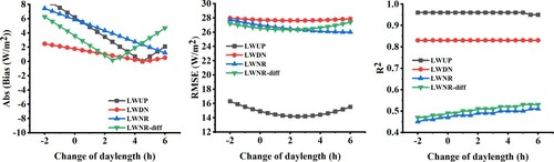
The linear sinusoidal interpolation method was used to investigate the effect of day length on the daily LW radiation estimates. Figure 17 shows the variations of the daily LW radiation estimate accuracies with changes of day length. The variations of the accuracy of the LW radiation with respect to day length were not consistent. For example, the bias of LWNR decreased with day length, while there were obvious inflection points in the biases for LWUP, LWDN, and LWNR-diff, but the positions of the inflection point were different. Hence, we choose to increase the day length by 1.5 h. Overall, the accuracy of the estimated surface daily LW radiation was better than those without extending the day length. We added 1.5 h to the day length to calculate the daily LW radiation. The R², bias and RMSE were 0.97, −4.15 and 13.74 W/m² for the daily LWUP, respectively; 0.84, −1.3 and 27.52 W/m² for the daily LWDN, respectively; 0.5, 4.52 and 26.29 W/m² for the LWNR, respectively; and were 0.52, 2.85 and 25.91 W/m² for the LWNR-diff, respectively. Compared to Figure 7, the accuracies of the daily LW radiation were improved when the day length was increased by 1.5 h which contrasts with the results of daily SW and NR or PAR estimates (Bisht et al. 2005; Bisht and Bras 2010; Wang et al. 2010). If the 1.5 h day length increased surface daily LW radiation were employed to calculate surface monthly LW radiation, the accuracies were also improved, with a bias/RMSE of −3.59/10.5 W/m² for monthly LWUP, −1.5/15.33 W/m² for monthly LWDN, 3.72/13.39 W/m² for monthly LWNR, and 2.09/12.93 W/m² for monthly LWNR-diff. Compared with the Figure 9, both absolute values of bias and RMSEs were reduced.

Figure 17. Relationships between day length and the accuracy of the estimated daily LW radiation in terms of, bias, RMSE and R².

4.3. Accuracy of daily LW radiation under clear-sky and cloudy-sky conditions

Usually, daily averaged SW or R_n is calculated separately under clear-sky and cloudy-sky conditions or is only calculated under clear-sky conditions (Lagouarde et al. 1991; Bisht and Bras 2010; Long, Gao, and Singh 2010; Wang et al. 2010; Hou et al. 2014; Carmona, Rivas, and Caselles 2015; Yan et al. 2018). Here, we investigated the accuracy of daily surface LW radiation estimates under clear-sky and cloudy-sky conditions. A given pixel is only labeled as clear sky when the GLASS LW radiation observations are all confidently clear; a pixel is only labeled as cloudy sky when GLASS LW radiation observations are all confidently cloudy. The time extension method used was the linear sine interpolation method. Note that probably clear and uncertain conditions were not included.

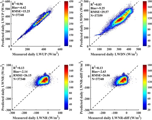
Figure 18 shows the clear-sky estimation results for daily surface LW radiation. The R², bias and RMSE were 0.98, −4.85 and 11.31 W/m² for the daily LWUP, respectively; 0.86, 0.12 and 24.96 W/m² for the daily LWDN, respectively; were 0.55, 7.63, 25.11 W/m² for the daily LWNR and 0.56, 4.68, 24.43 W/m² daily LWNR-diff, respectively. These results were obvious better than those presented in Figure 7 which are the combined results for confidently clear, probably clear, confidently cloudy and probably cloudy conditions, except the daily LWNR. It showed that the results under clear condition were better than those of all-sky condition. The accuracies of daily LW radiation under cloudy-sky conditions are shown in Figure 19. The results of dailt LWUP and LWDN were worse than those presented in Figure 10, because the accuracy of cloudy-sky instantaneous LW radiation is worse than that under clear-sky conditions, as we can see from Section 3.1. The R², bias and RMSE were 0.96, −6.62 and 15.25 W/m², respectively, for the daily LWUP; 0.83, −9.25 and 29.57 W/m², respectively, for the daily LWDN; 0.13, −2.14 and 26.15 W/m², respectively for the daily LWNR; and 0.13, −2.63 W/m²; and 26.06 W/m² for daily diff LWNR.

Figure 18. Accuracies of estimated daily LWUP, LWDN, LWNR and diff LWNR under clear-sky conditions.

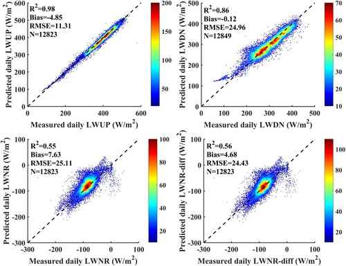
Figure 19. Accuracies of estimated daily LWUP, LWDN, LWNR and diff LWNR under cloudy-sky conditions.

5. Conclusions

The daily averaged surface LW radiation or diurnal cycle of surface LW radiation is required by agricultural, hydrological and meteorological models. High spatial resolution long-term daily surface LW radiation products are currently unavailable. High spatial resolution daily LW radiation levels were estimated from the instantaneous GLASS LW product by using the time extension methods in this study.

Four time extension methods were evaluated by ground measurements that were collocated with the overpass times of GLASS LW radiation. They all achieved accurate estimates of the daily LW radiation. The biases were close to zero and the RMSEs are less than or approximate to 10 W/m² for the daily LW radiation estimate. The linear sine interpolation method performed slightly better than the other three methods. When the time extension methods were applied to the GLASS LW product, the limited numbers of observations could not adequately capture the diurnal variations in the surface LW radiation. The linear sine interpolation performed best with a bias/RMSE of −6.30/15.10 W/m² for the daily LWUP, −1.65/27.63 W/m² for the daily LWDN, and 6.17/26.91 W/m² for the daily LWNR. The bias and RMSE of LWNR-diff were 4.69 and 26.42 W/m², respectively. The daily LW radiation estimated by the linear sine interpolation method were averaged to obtain the surface monthly LW radiation. The bias/RMSE were −6.29/11.84 W/m2 for the monthly LWUP, −1.75/15.94 W/m² for the monthly LWDN, 6.14/15.31 W/m2 for the monthly LWNR, and 4.64/15.65 W/m² for the monthly LWNR-diff. The performances of the four time extension methods were also investigated for different latitude regions (e.g. high-latitude, mid-latitude and low-latitude). The discrepancies among the four interpolation methods were generally small. Due to the greater disparity in sample numbers, the accuracies for the mid-latitudes were similar to those derived from globally distributed samples. The efficacy of an increment in overpass times for high-latitude regions was not significant.

The accuracy of GLASS LW radiation affects the simulated diurnal cycle of LW radiation and therefore the estimated daily values. We established the linear relationship between the GLASS LW radiation and site-measured LW radiation and adjusted the GLASS LW radiation with the established linear relationship. The RMSE of the daily LW radiation which was estimated by the linear sine interpolation method was improved but the bias was slightly degraded except for daily LWDN. The bias/RMSE was −7.39/9.85 W/m² for the daily LWUP; −4.1/16.06 W/m² for the daily LWDN; 7.53/17.84 W/m² for the daily LWNR; and 4.23/14.13 W/m² for the daily LWNR-diff. The overestimate or underestimate phenomena of surface daily LW radiation estimates were obviously improved if bias removal was used to adjust the GLASS LW radiation. The bias/RMSE was −0.31/12.97 W/m² for the daily LWUP; −0.96/27.75 W/m² for the daily LWDN; 0.3/26.17 W/m² for the daily LWNR; and −0.51/25.97 W/m² for the daily LWNR-diff. Both methods cannot fully improve the accuracy of the estimated surface daily LW radiation. We found that the length of the diurnal cycle of LW radiation was longer than that of shortwave radiation by using site measurements and that day length affects the accuracy of daily LW radiation calculations. We proposed lengthening the day length by 1.5 h and the accuracy of daily LW radiation slightly improved. The bias/RMSE were −4.15/13.74 W/m² for the daily LWUP, −1.3/27.52 W/m² for the daily LWDN, 4.52/26.29 W/m² for the LWNR, and 2.85/25.91 W/m² for the LWNR-diff, respectively. When the day length increased surface LW radiation were used to calculate monthly LW radiation, the accuracy were also improved. The bias/RMSE of were −3.59/10.5 W/m² for monthly LWUP, −1.5/15.33 W/m² for monthly LWDN, 3.72/13.39 W/m² for monthly LWNR, and 2.09/12.93 W/m² for monthly LWNR-diff, respectively.

Combining the day length adjustment and linear sine interpolation method, we are producing a long-term daily LW radiation product from the GLASS LW product. This product will be freely released to public in the near future.

Acknowledgment

This work was supported by the National Key Research and Development Program of China under Grant 2016YFA0600101, National Natural Science Foundation of China via grants 42090011, 41771365 and 42071308, and the Second Tibetan Plateau Scientific Expedition and Research Program (STEP) under Grant 2019QZKK0206.

Disclosure statement

No potential conflict of interest was reported by the author(s).

Data availability statement

Table

Name	URL
GLASS longwave radiation product	http://www.glass.umd.edu/
	http://www.geodata.cn/thematicView/GLASS.html
AsiaFlux data	http://asiaflux.net/
AmeriFlux data	https://ameriflux.lbl.gov/
BSRN data	https://bsrn.awi.de/
CEOP data	https://www.eol.ucar.edu/field_projects/ceop

Additional information

Funding

This work was supported by the National Key Research and Development Program of China under [grant number 2016YFA0600101], National Natural Science Foundation of China via [grant numbers 42090011, 41771365, and 42071308], and the Second Tibetan Plateau Scientific Expedition and Research Program (STEP) under [grant number 2019QZKK0206].

References

- Allen, Richard G, Luis S Pereira, Dirk Raes, and Martin Smith. 1998. “FAO Irrigation and Drainage Paper No. 56. Crop Evapotranspiration (Guidelines for Computing Crop Water Requirements).” Review of. Food and Agriculture Organisation of the United Nations, Rome 300.
- Allen, R. G., R. Trezza, and M. Tasumi. 2006. “Analytical Integrated Functions for Daily Solar Radiation on Slopes.” In Handbook of Environmental Chemistry, Volume 5: Water Pollution, 55–73.
- Baldocchi, Dennis, Eva Falge, Lianhong Gu, Richard Olson, David Hollinger, Steve Running, Peter Anthoni, Ch Bernhofer, Kenneth Davis, and Robert Evans. 2001. “FLUXNET: A New Tool to Study the Temporal and Spatial Variability of Ecosystem-Scale Carbon Dioxide, Water Vapor, and Energy Flux Densities.” Review of. Bulletin of the American Meteorological Society 82 (11): 2415–34.
- Bastiaanssen, W. G. M. 2000. “SEBAL-based Sensible and Latent Heat Fluxes in the Irrigated Gediz Basin, Turkey.” Review of. Journal of Hydrology 229 (1-2): 87–100. doi:https://doi.org/10.1016/S0022-1694(99)00202-4.
- Bisht, Gautam, and Rafael L. Bras. 2010. “Estimation of Net Radiation from the MODIS Data Under all Sky Conditions: Southern Great Plains Case Study.” Review of. Remote Sensing of Environment 114 (7): 1522–34. doi:https://doi.org/10.1016/j.rse.2010.02.007.
- Bisht, Gautam, and Rafael L. Bras. 2011. “Estimation of Net Radiation from the Moderate Resolution Imaging Spectroradiometer Over the Continental United States.” Review of. Ieee Transactions on Geoscience and Remote Sensing 49 (6): 2448–62. doi:https://doi.org/10.1109/tgrs.2010.2096227.
- Bisht, Gautam, Virginia Venturini, Shafiqul Islam, and Le Jiang. 2005. “Estimation of the Net Radiation Using MODIS (Moderate Resolution Imaging Spectroradiometer) Data for Clear Sky Days.” Review of. Remote Sensing of Environment 97 (1): 52–67. doi:https://doi.org/10.1016/j.rse.2005.03.014.
- Brooks, D. R., and P. Minnis. 1984. “Comparison of Longwave Diurnal Models Applied to Simulations of the Earth Radiation Budget Experiment.” Review of. Journal of Climate and Applied Meteorology 23 (1984): 155–60.
- Brunt, David. 1932. “Notes on Radiation in the Atmosphere. I.” Review of. Quarterly Journal of the Royal Meteorological Society 58 (247): 389–420.
- Brutsaert, W. 1975. “On a Derivable Formula for Long-Wave Radiation from Clear Skies.” Review of. Water Resources Research 11 (5): 742–4. doi:https://doi.org/10.1029/WR011i005p00742.
- Carmona, Facundo, Raúl Rivas, and Vicente Caselles. 2014. “Estimation of Daytime Downward Longwave Radiation Under Clear and Cloudy Skies Conditions Over a Sub-Humid Region.” Review of. Theoretical and Applied Climatology 115 (1-2): 281–95.
- Carmona, Facundo, Raul Rivas, and Vicente Caselles. 2015. “Development of a General Model to Estimate the Instantaneous, Daily, and Daytime net Radiation with Satellite Data on Clear-Sky Days.” Review of. Remote Sensing of Environment 171: 1–13. doi:https://doi.org/10.1016/j.rse.2015.10.003.
- Cheng, Jie, and Shunlin Liang. 2014. “Estimating the Broadband Longwave Emissivity of Global Bare Soil from the MODIS Shortwave Albedo Product.” Review of. Journal of Geophysical Research: Atmospheres 119 (2): 614–34. doi:https://doi.org/10.1002/2013jd020689.
- Cheng, Jie, and Shunlin Liang. 2016. “Global Estimates for High-Spatial-Resolution Clear-Sky Land Surface Upwelling Longwave Radiation from MODIS Data.” Review of. Ieee Transactions on Geoscience and Remote Sensing 54 (7): 4115–29. doi:https://doi.org/10.1109/tgrs.2016.2537650.
- Cheng, Jie, Shunlin Liang, Wout Verhoef, Linpeng Shi, and Qiang Liu. 2016. “Estimating the Hemispherical Broadband Longwave Emissivity of Global Vegetated Surfaces Using a Radiative Transfer Model.” Review of. Ieee Transactions on Geoscience and Remote Sensing 54 (2): 905–17. doi:https://doi.org/10.1109/tgrs.2015.2469535.
- Cheng, Jie, Shunlin Liang, Wenhui Wang, and Yamin Guo. 2017. “An Efficient Hybrid Method for Estimating Clear-sky Surface Downward Longwave Radiation from MODIS Data.” Review of. Journal of Geophysical Research-Atmospheres 122 (5): 2616–30. doi:https://doi.org/10.1002/2016jd026250.
- Cheng, Jie, Feng Yang, and Yamin Guo. 2019. “A Comparative Study of Bulk Parameterization Schemes for Estimating Cloudy-Sky Surface Downward Longwave Radiation.” Review of. Remote Sensing 11 (5), doi:https://doi.org/10.3390/rs11050528.
- Christensen, O. B., J. H. Christensen, B. Machenhauer, and M. Ole B Botzet. 1998. “Very High-Resolution Regional Climate Simulations Over Scandinavia—Present Climate.” Review of. Journal of Climate 11 (12): 3204–29.
- Crawford, Todd M, and Claude E Duchon. 1999. “An Improved Parameterization for Estimating Effective Atmospheric Emissivity for Use in Calculating Daytime Downwelling Longwave Radiation.” Review of. Journal of Applied Meteorology 38 (4): 474–80.
- Diak, George R, William L Bland, John R Mecikalski, and Martha C Anderson. 2000. “Satellite-based Estimates of Longwave Radiation for Agricultural Applications.” Review of. Agricultural and Forest Meteorology 103 (4): 349–55.
- Doelling, David R, Norman G Loeb, Dennis F Keyes, Michele L Nordeen, Daniel Morstad, Cathy Nguyen, Bruce A Wielicki, David F Young, and Moguo Sun. 2013. “Geostationary Enhanced Temporal Interpolation for CERES Flux Products.” Review of. Journal of Atmospheric and Oceanic Technology 30 (6): 1072–90.
- Doelling, David R, Moguo Sun, Le Trang Nguyen, Michele L Nordeen, Conor O Haney, Dennis F Keyes, and Pamela E Mlynczak. 2016. “Advances in Geostationary-Derived Longwave Fluxes for the CERES Synoptic (SYN1deg) Product.” Review of. Journal of Atmospheric and Oceanic Technology 33 (3): 503–21.
- Dongdong, Wang, Liang Shunlin, He Tao, and Shi Qinqing. 2015. “Estimation of Daily Surface Shortwave Net Radiation From the Combined MODIS Data.” Review of. Ieee Transactions on Geoscience and Remote Sensing 53 (10): 5519–29. doi:https://doi.org/10.1109/tgrs.2015.2424716.
- Duarte, Henrique Ferro, Nelson Luís Dias, and Selma Regina Maggiotto. 2006. “Assessing Daytime Downward Longwave Radiation Estimates for Clear and Cloudy Skies in Southern Brazil.” Review of. Agricultural and Forest Meteorology 139 (3-4): 171–81.
- Ellingson, Robert G, and Mamoudou B Ba. 2003. “A Study of Diurnal Variation of OLR from the GOES Sounder.” Review of. Journal of Atmospheric and Oceanic Technology 20 (1): 90–8.
- Forman, B. A., and S. A. Margulis. 2007. “Estimates of Total Downwelling Surface Radiation Using a High-resolution GOES-based Cloud Product Along with MODIS and AIRS Products.” Review of.
- Forman, B. A., and S. A. Margulis. 2009. “High-resolution Satellite-Based Cloud-Coupled Estimates of Total Downwelling Surface Radiation for Hydrologic Modelling Applications.” Review of. Hydrology and Earth System Sciences 13 (7): 969–86. doi:https://doi.org/10.5194/hess-13-969-2009.
- Göttsche, F. M., F. S. Olesen, I. F. Trigo, A. Bork-Unkelbach, and M. A. Martin. 2016. “Long Term Validation of Land Surface Temperature Retrieved from MSG/SEVIRI with Continuous in-Situ Measurements in Africa.” Review of. Remote Sensing 8 (5): 410.
- Gui, Sheng, Shunlin Liang, and Lin Li. 2010. “Evaluation of Satellite-Estimated Surface Longwave Radiation Using Ground-Based Observations.” Review of. Journal of Geophysical Research 115 (D18), doi:https://doi.org/10.1029/2009jd013635.
- Guo, Yamin, Jie Cheng, and Shunlin Liang. 2019. “Comprehensive Assessment of Parameterization Methods for Estimating Clear-sky Surface Downward Longwave Radiation.” Review of. Theoretical and Applied Climatology 135 (3): 1045–58. doi:https://doi.org/10.1007/s00704-018-2423-7.
- Gupta, S. K., W. L. Darnell, and A. C. Wilber. 1992. “A Parameterization For Longwave Surface Radiation from Satellite Data - Recent Improvements.” Review of. Journal of Applied Meteorology 31 (12): 1361–7. doi:https://doi.org/10.1175/1520-0450(1992)031<1361:apflsr>2.0.co;2.
- Gupta, Shashi K., David P. Kratz, Paul W. Stackhouse, Anne C. Wilber, Taiping Zhang, and Victor E. Sothcott. 2010. “Improvement of Surface Longwave Flux Algorithms Used in CERES Processing.” Review of. Journal of Applied Meteorology and Climatology 49 (7): 1579–89. doi:https://doi.org/10.1175/2010jamc2463.1.
- Hou, J., G. Jia, T. Zhao, H. Wang, and B. Tang. 2014. “Satellite-based Estimation of Daily Average Net Radiation Under Clear-sky Conditions.” Review of. Advances in Atmospheric Sciences 31 (3): 705–20.
- Hu, Tian, Luigi J. Renzullo, Biao Cao, Albert I. J. M. van Dijk, Yongming Du, Hua Li, Jie Cheng, Zhihong Xu, Jun Zhou, and Qinhuo Liu. 2019. “Directional Variation in Surface Emissivity Inferred from the MYD21 Product and its Influence on Estimated Surface Upwelling Longwave Radiation.” Review of. Remote Sensing of Environment 228: 45–60. doi:https://doi.org/10.1016/j.rse.2019.04.012.
- Hwang, Kyotaek, Minha Choi, Seung Oh Lee, and Jong-Won Seo. 2013. “Estimation of Instantaneous and Daily Net Radiation from MODIS Data Under Clear Sky Conditions: A Case Study in East Asia.” Review of. Irrigation Science 31 (5): 1173–84. doi:https://doi.org/10.1007/s00271-012-0396-3.
- Irmak, Suat, Lameck O. Odhiambo, and Denis Mutiibwa. 2011. “Evaluating the Impact of Daily Net Radiation Models on Grass and Alfalfa-Reference Evapotranspiration Using the Penman-Monteith Equation in a Subhumid and Semiarid Climate.” Review of. Journal of Irrigation and Drainage Engineering 137 (2): 59–72. doi:https://doi.org/10.1061/(asce)ir.1943-4774.0000278.
- Journée, Michel, and Cédric Bertrand. 2010. “Improving the Spatio-Temporal Distribution of Surface Solar Radiation Data by Merging Ground and Satellite Measurements.” Review of. Remote Sensing of Environment 114 (11): 2692–704.
- Kratz, David P., Shashi K. Gupta, Anne C. Wilber, and Victor E. Sothcott. 2020. “Validation of the CERES Edition-4A Surface-Only Flux Algorithms.” Review of. Journal of Applied Meteorology and Climatology 59 (2): 281–95. doi:https://doi.org/10.1175/JAMC-D-19-0068.1.
- Lagouarde, Jean-Pierre, and Yves Brunet. 1993. “A Simple Model for Estimating the Daily Upward Longwave Surface Radiation Flux from NOAA-AVHRR Data.” Review of. International Journal of Remote Sensing 14 (5): 907–25.
- Lagouarde, J. P., Y. Brunet, Y. Kerr, and J. Imbernon. 1991. “Estimating the Daily Upward Longwave Radiation from NOAA-AVHRR Data for Mapping net Radiation.” Review of. Advances in Space Research 11 (3): 151–61.
- Liang, S., J. Cheng, K. Jia, B. Jiang, Q. Liu, Z. Xiao, Y. Yao, et al. 2021. “The Global Land Surface Satellite (GLASS) Product Suite.” Review of. Bulletin of the American Meteorological Society 102 (2): E323–E37.
- Liang, Shunlin, Dongdong Wang, Tao He, and Yueyun Yu. 2019. “Remote Sensing of Earth's Energy Budget: Synthesis and Review.” Review of. International Journal of Digital Earth 12 (7): 737–780.
- Liang, Shunlin, Xiang Zhao, Suhong Liu, Wenping Yuan, Xiao Cheng, Zhiqiang Xiao, Xiaotong Zhang, Qiang Liu, Jie Cheng, and Hairong Tang. 2013. “A Long-Term Global LAnd Surface Satellite (GLASS) Data-set for Environmental Studies.” Review of. International Journal of Digital Earth 6 (sup1): 5–33.
- Liu, Shaomin, Ziwei Xu, Lisheng Song, Qianyi Zhao, Ge Yong, Tongren Xu, Yanfei Ma, Zhongli Zhu, Zhenzhen Jia, and Fen Zhang. 2016. “Upscaling Evapotranspiration Measurements from Multi-Site to the Satellite Pixel Scale Over Heterogeneous Land Surfaces.” Review of. Agricultural & Forest Meteorology 230: 97–113.
- Loeb, N. G., B. A. Wielicki, T. Wong, and P. A. Parker. 2009. “Impact of Data Gaps on Satellite Broadband Radiation Records.” Review of. Journal of Geophysical Research Atmospheres 114 (11), doi:https://doi.org/10.1029/2008JD011183.
- Long, Di, Yanchun Gao, and Vijay P. Singh. 2010. “Estimation of Daily Average net Radiation from MODIS Data and DEM Over the Baiyangdian Watershed in North China for Clear sky Days.” Review of. Journal of Hydrology 388 (3-4): 217–33. doi:https://doi.org/10.1016/j.jhydrol.2010.04.042.
- Meeus, Jean. 1991. Astronomical Algorithms. Richmond, VA: Willmann-Bell.
- Minnis, P., and E. F. Harrison. 1984. “Diurnal Variability of Regional Cloud and Clear-sky Radiative Parameters Derived from GOES Data. Part I: Analysis Method.” Review of. Journal of Climate & Applied Meteorology 23 (7): 993–1011. doi:https://doi.org/10.1175/1520-0450(1984)023<0993:DVORCA>2.0.CO;2.
- Ohmura, A., E. G. Dutton, B. Forgan, C. Fröhlich, H. Gilgen, H. Hegner, A. Heimo, et al. 1998. “Baseline Surface Radiation Network (BSRN/WCRP): New Precision Radiometry for Climate Research.” Review of. Bulletin of the American Meteorological Society 79 (10): 2115–36. doi:https://doi.org/10.1175/1520-0477(1998)079<2115:BSRNBW>2.0.CO;2.
- Olofsson, Pontus, and Lars Eklundh. 2007. “Estimation of Absorbed PAR Across Scandinavia from Satellite Measurements. Part II: Modeling and Evaluating the Fractional Absorption.” Review of. Remote Sensing of Environment 110 (2): 252–61.
- Ortega-Farias, Samuel, Rodrigo Antonioletti, and Albert Olioso. 2000. “Net Radiation Model Evaluation at an Hourly Time Step for Mediterranean Conditions.” Review of. Agronomie 20 (2): 157–64.
- Penman, H. L. 1948. “Natural Evaporation from Open Water, Bare Soil and Grass.” Review of. Proceedings of the Royal Society of London 193 (1032): 120–45.
- Philipona, Rolf, Claus Fröhlich, Klaus Dehne, John DeLuisi, John Augustine, Ellsworth Dutton, Don Nelson, Bruce Forgan, Peter Novotny, and John Hickey. 1998. “The Baseline Surface Radiation Network Pyrgeometer Round-Robin Calibration Experiment.” Review of. Journal of Atmospheric and Oceanic Technology 15 (3): 687–96.
- Pinker, R. T., J. D. Tarpley, I. Laszlo, K. E. Mitchell, P. R. Houser, E. F. Wood, J. C. Schaake, et al. 2003. “Surface Radiation Budgets in Support of the GEWEX Continental-Scale International Project (GCIP) and the GEWEX Americas Prediction Project (GAPP), Including the North American Land Data Assimilation System (NLDAS) Project.” Review of. Journal of Geophysical Research-Atmospheres 108 (D22), doi:https://doi.org/10.1029/2002jd003301.
- Prata, A. J. 1996. “A New Long-Wave Formula for Estimating Downward Clear-sky Radiation at the Surface.” Review of. Quarterly Journal of the Royal Meteorological Society 122 (533): 1127–51.
- Qin, Boxiong, Biao Cao, Hua Li, Zunjian Bian, Tian Hu, Yongming Du, Yingpin Yang, Qing Xiao, and Qinhuo Liu. 2020. “Evaluation of Six High-Spatial Resolution Clear-Sky Surface Upward Longwave Radiation Estimation Methods with MODIS.” Review of. Remote Sensing 12 (11): 1834.
- Roupioz, Laure, Li Jia, Francoise Nerry, and Massimo Menenti. 2016. “Estimation of Daily Solar Radiation Budget at Kilometer Resolution Over the Tibetan Plateau by Integrating MODIS Data Products and a DEM.” Review of. Remote Sensing 8 (6), doi:https://doi.org/10.3390/rs8060504.
- Rutan, David A., Seiji Kato, David R. Doelling, Fred G. Rose, Le Trang Nguyen, Thomas E. Caldwell, and Norman G. Loeb. 2015. “CERES Synoptic Product: Methodology and Validation of Surface Radiant Flux.” Review of. Journal of Atmospheric and Oceanic Technology 32 (6): 1121–43. doi:https://doi.org/10.1175/jtech-d-14-00165.1.
- Samani, Z., S. A. Bawazir, M. Bleiweiss, R. Skaggs, and V. D. Tran. 2007. “Estimating Daily Net Radiation Over Vegetation Canopy Through Remote Sensing and Climatic Data.” Review of. Journal of Irrigation and Drainage Engineering 133 (4): 291–7. doi:https://doi.org/10.1061/(ASCE)0733-9437(2007)133:4(291).
- Swinbank, W. C. Q. J. R. 1963. “Long-wave Radiation from Clear Skies.” Review of. Quarterly Journal of the Royal Meteorological Society 89 (381): 339–48.
- Tang, Bohui, and Zhao-Liang Li. 2008. “Estimation of Instantaneous Net Surface Longwave Radiation from MODIS Cloud-Free Data.” Review of. Remote Sensing of Environment 112 (9): 3482–92.
- Trenberth, Kevin E., John T. Fasullo, and Jeffrey Kiehl. 2009. “Earth's Global Energy Budget.” Review of. Bulletin of the American Meteorological Society 90 (3): 311–24. doi:https://doi.org/10.1175/2008BAMS2634.1.
- Wang, Kaicun, and Robert E Dickinson. 2013. “Global Atmospheric Downward Longwave Radiation at the Surface from Ground-Based Observations, Satellite Retrievals, and Reanalyses.” Review of. Reviews of Geophysics 51 (2): 150–85.
- Wang, Wenhui, and Shunlin Liang. 2009. “Estimation of High-Spatial Resolution Clear-sky Longwave Downward and net Radiation Over Land Surfaces from MODIS Data.” Review of. Remote Sensing of Environment 113 (4): 745–54. doi:https://doi.org/10.1016/j.rse.2008.12.004.
- Wang, Dongdong, Shunlin Liang, Ronggao Liu, and Tao Zheng. 2010. “Estimation of Daily-Integrated PAR from Sparse Satellite Observations: Comparison of Temporal Scaling Methods.” Review of. International Journal of Remote Sensing 31 (6): 1661–77.
- Wang, Wenhui, Shunlin Liang, and Tilden Meyers. 2008. “Validating MODIS Land Surface Temperature Products Using Long-Term Nighttime Ground Measurements.” Review of. Remote Sensing of Environment 112 (3): 623–35.
- Wang, Tianxing, and Ya Ma. 2019. “Cloudy-Sky Land Surface Longwave Upward Radiation Derivation from Satellite Measurements.” Paper presented at the IGARSS 2019-2019 IEEE International Geoscience and Remote Sensing Symposium.
- Wang, T., Y. Ma, and J. Shi. 2019. “Cloudy-Sky Land Surface Longwave Upward Radiation Derivation from Satellite Measurements.” Paper presented at the IGARSS 2019 - 2019 IEEE International Geoscience and Remote Sensing Symposium.
- Wang, Jiao, Bo-Hui Tang, Xiao-Yu Zhang, Hua Wu, and Zhao-Liang Li. 2014. “Estimation of Surface Longwave Radiation Over the Tibetan Plateau Region Using MODIS Data for Cloud-Free Skies.” Review of. Ieee Journal of Selected Topics in Applied Earth Observations and Remote Sensing 7 (9): 3695–703. doi:https://doi.org/10.1109/jstars.2014.2320585.
- Wenhui, Wang, Liang Shunlin, and J. A. Augustine. 2009. “Estimating High Spatial Resolution Clear-Sky Land Surface Upwelling Longwave Radiation From MODIS Data.” Review of. Ieee Transactions on Geoscience and Remote Sensing 47 (5): 1559–70. doi:https://doi.org/10.1109/tgrs.2008.2005206.
- Wild, M., A. Ohmura, H. Gilgen, J. J. Morcrette, and A. Slingo. 2001. “Evaluation of Downward Longwave Radiation in General Circulation Model.” Review of. Journal of Climate 14 (15): 3227–39.
- Xu, Xiaojun, Huaqiang Du, Guomo Zhou, Fangjie Mao, Pingheng Li, Weiliang Fan, and Dien Zhu. 2016. “A Method for Daily Global Solar Radiation Estimation from Two Instantaneous Values Using MODIS Atmospheric Products.” Review of. Energy 111: 117–25.
- Xu, Ziwei, Shaomin Liu, Li Xin, Shengjin Shi, Jiemin Wang, Zhongli Zhu, Tongren Xu, Weizhen Wang, and Mingguo Ma. 2013. “Intercomparison of Surface Energy Flux Measurement Systems Used During the HiWATER-MUSOEXE.” Review of. Journal of Geophysical Research Atmospheres 118 (23): 13–157.
- Yan, Guangjian, Yiyi Tong, Kai Yan, Xihan Mu, Qing Chu, Yingji Zhou, Yanan Liu, et al. 2018. “Temporal Extrapolation of Daily Downward Shortwave Radiation Over Cloud-Free Rugged Terrains. Part 1: Analysis of Topographic Effects.” Review of. Ieee Transactions on Geoscience and Remote Sensing 56 (11): 6375–94. doi:https://doi.org/10.1109/tgrs.2018.2838143.
- Yang, Feng, and Jie Cheng. 2020. “A Framework for Estimating Cloudy Sky Surface Downward Longwave Radiation from the Derived Active and Passive Cloud Property Parameters.” Review of. Remote Sensing of Environment 248: 111972. doi:https://doi.org/10.1016/j.rse.2020.111972.
- Young, D. F., P. Minnis, D. R. Doelling, G. G. Gibson, and T. Wong. 1998. “Temporal Interpolation Methods for the Clouds and the Earth's Radiant Energy System (CERES) Experiment.” Review of. Journal of Applied Meteorology 37 (6): 572–90. doi:https://doi.org/10.1175/1520-0450(1998)037<0572:TIMFTC>2.0.CO;2.
- Yu, Y., Y. Liu, P. Yu, Y. Liu, and P. Yu. 2018. “Land Surface Temperature Product Development for JPSS and GOES-R Missions.” Review of. Comprehensive Remote Sensing 5: 284–303.
- Zeng, Qi, Jie Cheng, and Lixin Dong. 2020. “Assessment of the Long-Term High-Spatial-Resolution Global LAnd Surface Satellite (GLASS) Surface Longwave Radiation Product Using Ground Measurements.” Review of. Ieee Journal of Selected Topics in Applied Earth Observations and Remote Sensing 13: 2032–55.
- Zhang, Yuanchong, William B Rossow, Andrew A Lacis, Valdar Oinas, and Michael I Mishchenko. 2004. “Calculation of Radiative Fluxes from the Surface to Top of Atmosphere Based on ISCCP and Other Global Data Sets: Refinements of the Radiative Transfer Model and the Input Data.” Review of. Journal of Geophysical Research: Atmospheres 109 (D19): 1–27.
- Zhang, Yuanchong, William B Rossow, and Paul W Stackhouse Jr 2007. “Comparison of Different Global Information Sources Used in Surface Radiative Flux Calculation: Radiative Properties of the Surface.” Review of. Journal of Geophysical Research: Atmospheres 112 (D1): 1–20.
- Zhao, Ping, Xiangde Xu, Fei Chen, Xueliang Guo, Xiangdong Zheng, Liping Liu, Yang Hong, et al. 2018. “The Third Atmospheric Scientific Experiment for Understanding the Earth–Atmosphere Coupled System Over the Tibetan Plateau and Its Effects.” Review of. Bulletin of the American Meteorological Society 99 (4): 757–76. doi:https://doi.org/10.1175/BAMS-D-16-0050.1.
- Zhou, Shugui, and Jie Cheng. 2018. “Estimation of High Spatial-Resolution Clear-Sky Land Surface-Upwelling Longwave Radiation from VIIRS/S-NPP Data.” Review of. Remote Sensing 10 (2), doi:https://doi.org/10.3390/rs10020253.
- Zhou, Yaping, David P. Kratz, Anne C. Wilber, Shashi K. Gupta, and Robert D. Cess. 2007. “An Improved Algorithm for Retrieving Surface Downwelling Longwave Radiation from Satellite Measurements.” Review of. Journal of Geophysical Research 112 (D15), doi:https://doi.org/10.1029/2006jd008159.
- Zhou, Yingji, Guangjian Yan, Jing Zhao, Qing Chu, Yanan Liu, Kai Yan, Yiyi Tong, Xihan Mu, Donghui Xie, and Wuming Zhang. 2018. “Estimation of Daily Average Downward Shortwave Radiation Over Antarctica.” Review of. Remote Sensing 10 (3), doi:https://doi.org/10.3390/rs10030422.