Fine scale optical remote sensing experiment of mixed stand over complex terrain (FOREST) in the Genhe Reserve Area: objective, observation and a case study

ABSTRACT

Optical remote sensing allows to efficiently monitor forest ecosystems at regional and global scales. However, most of the widely used optical forward models and backward estimation methods are only suitable for forest canopies in flat areas. To evaluate the recent progress in forest remote sensing over complex terrain, a satellite-airborne-ground synchronous Fine scale Optical Remote sensing Experiment of mixed Stand over complex Terrain (FOREST) was conducted over a 1 km×1 km key experiment area (KEA) located in the Genhe Reserve Areain 2016. Twenty 30 m×30 m elementary sampling units (ESUs) were established to represent the spatiotemporal variations of the KEA. Structural and spectral parameters were simultaneously measured for each ESU. As a case study, we first built two 3D scenes of the KEA with individual-tree and voxel-based approaches, and then simulated the canopy reflectance using the LargE-Scale remote sensing data and image Simulation framework over heterogeneous 3D scenes (LESS). The correlation coefficient between the LESS-simulated reflectance and the airborne-measured reflectance reaches 0.68–0.73 in the red band and 0.56–0.59 in the near-infrared band, indicating a good quality of the experiment dataset. More validation studies of the related forward models and retrieval methods will be done.

KEYWORDS:

• Remote sensing experiment
• forest
• complex terrain
• Genhe Reserve Area
• LESS

1. Introduction

Forest ecosystems are crucial for the research of water, carbon and nutrient cycles, and are one of the most important ecosystems in the response to global climate change (Chen, 2021; Chmura et al. 2011; Geng et al. 2017). Numerous experiments have been carried out in forest canopies around the world for different research purposes. For example, Kuusk, Kuusk, and Lang (2009) introduced an experiment carried out at the Järvselja Training and Experimental Forestry District of Estonia to build a dataset for the validation of reflectance models in the fourth round of the RAdiative transfer Model Intercomparison (RAMI) (Widlowski et al. 2015). The goal of the Boreal Ecosystem-Atmosphere Study (BOREAS) (Sellers et al. 1997) is to improve the understanding of the interactions between the boreal forest biome and the atmosphere. The aim of NOPEX (Halldin et al. 1999), in the southern part of the European boreal zone, is to study energy, water and carbon exchanges. Surface moisture experiments have been usually based on active and passive microwave observations as reviewed by Zhao et al. (2020); however, optical remote sensing experiments have played an important role in forest ecosystem studies.

Remote sensing signals record the interaction results of the land surface and the energy emitted from the sun, ground, or the sensor itself (Cao et al. 2019; Gastellu-Etchegorry et al. 2017) and can be used to retrieve forest attribute parameters with the help of canopy models (Chen and Cihlar 1996; Ma et al. 2018). However, considering that many forests are located on rugged terrain (Wen et al. 2018), estimating forest attributes based on remote sensing is still challenging (Tian et al. 2015). For instance, the topographical effects lead to the occlusion of direct solar radiation and the obstruction from the surrounding topography for hemispherical diffuse skylight radiation. Rugged terrain significantly changes the solar-target-viewing geometry and complicates the radiative transfer process. In order to improve parameter estimation accuracy over rugged terrain, many bi-directional reflectance distribution function (BRDF)/directional brightness temperature (DBT) physical and kernel-driven models suitable for sloping ground or rugged terrain were developed (Cao et al. 2015; Hao et al. 2018; Wu et al. 2019). A comprehensive dataset of multi-scale observations over complex terrain is required to evaluate the progress of forest remote sensing in recent years.

The Greater Khingan Station is the only forest research station located in the cool temperature zone among the 17 national forest ecosystem research stations of China. The Greater Khingan Station is in the Genhe forestry reserve (120°12’ to 122°55’ E, 50°20’ to 52°30’ N), which belongs to the Hulunbeier League in Inner Mongolia. The site has a hilly topography with a mean altitude of approximately 1000 m. Occupying 75% of the total area, the forest is mainly composed of Larix gmelinii Rupr., Betula platyphylla Suk and Pinus sylvestris var. mongolica Litv. This station serves as a platform of forest meteorology, hydrology, productivity, health, carbon flux, water flux and global climate change research (Niu, Wang, and Wei 2013). Following the Complicate Observations and Multi-Parameter Land Information Constructions on Allied Telemetry Experiment (COMPLICATE) conducted in the Genhe Reserve Area in 2012–2013 (Tian et al. 2015), we carried out a Fine scale Optical Remote sensing Experiment of mixed Stand over complex Terrain (FOREST) in this region in 2016.

In the COMPLICATE experiment, light detection and ranging (LiDAR) data and charge coupled device (CCD) images for about 230 km² within the Genhe Reserve Area were obtained from August to September of 2012. However, in FOREST, all the observations are focused on the key experimentation area (KEA) with only 1 km ×1 km (corresponding with the spatial resolution of MODIS 1-km but not exactly overlapped with a MODIS pixel). FOREST was designed to synchronously obtain structural parameters (e.g. tree height, diameter at breast height (DBH), crown size, leaf size, plant area index (PAI), leaf area index (LAI), average leaf inclination angle (ALIA), fraction of vegetation cover (FVC) and clumping index (CI)) and spectral parameters (e.g. component reflectance, transmittance and temperature). The airborne LiDAR-CCD-Hyperspectral integrated mission (LiCHy) and Wide-angle Infrared Dual-mode line/area Array Scanner (WiDAS), and unmanned aerial vehicle (UAV) mounted hyperspectral, thermal infrared (TIR) and CCD sensors were implemented to bridge between fine-scale ground measurements and coarse-scale satellite observations.

Comparing with the former successful comprehensive experiments, for instance, Watershed Allied Telemetry Experimental Research (WATER) (Li et al. 2009), Heihe Watershed Allied Telemetry Experimental Research (HiWATER) (Li et al. 2013) and COMPLICATE (Tian et al. 2015), FOREST has three new features: (1) FOREST narrows the research object from a typical land surface (cropland, grassland, forest and so on) to that of a forest ecosystem; (2) the KEA region of FOREST is smaller (1 km ×1 km), making the fine-scale ground measurement become possible. Twenty elementary sampling units (ESUs) were established within the KEA to capture land surface heterogeneity. The ESU density is much higher than in the former comprehensive experiments; (3) UAV was introduced as one of the main observation approaches in FOREST. The spatial resolution of the images acquired by cameras mounted on the UAV can reach 0.1 m, supporting fine-scale remote sensing studies.

This manuscript is organized as follows. The detailed scientific objectives of this experiment are introduced in section 2. The airborne and UAV observations and the ground measurements are given in section 3 and 4 respectively. Section 5 presents a case study based on the FOREST dataset. Two 1 km × 1 km 3D scenes were reconstructed based on airborne LiCHy-LiDAR and ground measured properties, then, the LESS model simulated canopy reflectance was compared with LiCHy-Hyperspectral observations in red and near-infrared (NIR) bands for evaluating the quality of the FOREST dataset to some extent. The summary of the FOREST experiment is provided in the last section.

2. Scientific objectives

To evaluate the progress in forest remote sensing over rugged terrain, the FOREST experiment focused on following three scientific objectives. The first objective is to reconstruct an accurate large 3D forest scene over complex terrain using the dataset of airborne LiCHy and other in situ structural parameters to be used as a basis of optical models. Some efforts had been done to build realistic 3D forest scenes over large mountainous areas (Schneider et al. 2014). The second objective is to validate the BRDF physical models (Fan, Li, and Liu 2015; Wen et al. 2015; Wu et al. 2019; Xu et al. 2017; Yin et al. 2017), BRDF kernel-driven models (Hao et al. 2020, 2018; Jiao et al. 2016), DBT physical models (Bian et al. 2018; Cao et al. 2018) and DBT kernel-driven models (Cao et al. 2021; Hu et al. 2016) considering the remote sensing radiative and scattering mechanisms on complex terrain. The third objective is to validate forest parameter retrieval methods over rugged terrains, such as for PAI (Zou et al. 2018), LAI (Zhang et al., 2019a), FVC (Li et al. 2020), CI (Wei et al. 2019), canopy height (Wang et al. 2014), albedo (Peng et al. 2015), and leaf and background temperature (Bian et al. 2016). These three objectives allow us to better assess the current status and deficiencies of optical remote sensing over rugged terrain.

In order to achieve above scientific objectives, fine-scale ground measurement of structural and spectral parameters and coarse-resolution satellite observations were acquired (Figure 1). In addition, airborne and UAV observations were obtained to scale the observations from the ground to the satellites. Table 1 summarizes the experiment composition and measured parameters. The measurements were carried out according to five data quality control methods: (1) the instruments (e.g. LiCHy, WiDAS, UAV sensors and FLIR T440 camera) were calibrated before the measurement to ensure the radiation accuracy; (2) numerous artificial geometric targets were placed in the KEA to ensure the accuracy of the geometric correction; (3) the in situ measurement of each parameter was repeated several times to ensure sampling reliability (e.g. nine positions for each ESU and ten pictures for each position in the acquisition of Hemiview); (4) each instrument strictly followed its user manual (e.g. LAI-2000 was used during cloudy conditions whereas the TRAC was used on sunny days); (5) the measurements were completed within the shortest possible time to reduce the influence of solar zenith angle variation and surface temperature fluctuation.

Figure 1. Multi-scale observations in the FOREST experiment.

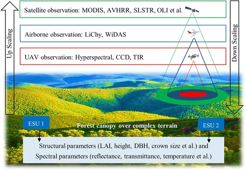
Table 1. Summary of the FOREST experiment composition and measured parameters.

Composition	Instruments	Description	Parameters
Airborne experiments	LiCHy	LiDAR, CCD, hyperspectral integrated system	Digital Surface Model (DSM), Digital Elevation Model (DEM), Canopy Height Model (CHM), Nadir hyperspectral reflectance
	WiDAS	Multi-spectral multi-angle integrated system	Multi-angle Multi-spectral reflectance, Multi-angle brightness temperature
UAV experiments	UAV-CCD	UAV + Sony A7	Reflectance
	UAV-Hyperspectral	UAV + Headwall	Nadir hyperspectral reflectance
	UAV-TIR	UAV + FLIR TAU640	Multi-angle brightness temperature
Ground experiments	Laser rangefinder	For structural parameter	Tree height
	Tape	For structural parameter	DBH, Crown size
	Li-3000	For structural parameter	Leaf size
	Tracing Radiation and Architecture of Canopies (TRAC)	For structural parameter	LAI, CI
	LAISmart	For structural parameter	LAI
	PocketLAI	For structural parameter	LAI
	LAI2000	For structural parameter	LAI, ALIA
	Hemiview	For structural parameter	LAI, ALIA, CI
	Terrestrial LiDAR	For structural parameter	LAI, ALIA, CI
	Nikon D3000	For structural parameter	FVC
	Integrating sphere	For spectral parameter	leaf reflectance
	ASD	For spectral parameter	leaf transmittance, background reflectance, bark reflectance
	FLIR T440	For spectral parameter	leaf temperature, background temperature, bark temperature

3. Airborne and UAV observations: design and results

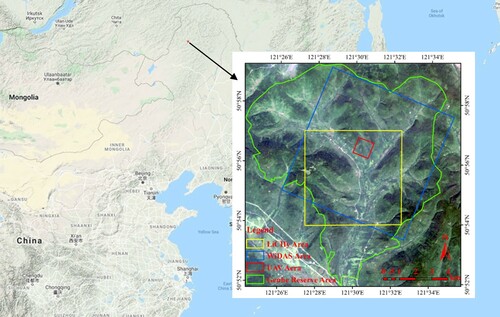
Figure 2 illustrates the location of the Genhe Reserve Area (see green polygon), the coverage of the airborne sensors (LiCHy with yellow polygon; WiDAS with blue polygon) and UAV sensors (including UAV-CCD, UAV-Hyperspectral and UAV-TIR, see the red polygon, i.e. KEA).

Figure 2. Coverage of airborne and UAV observations located in the Genhe Reserve Area.

3.1. LiDAR, CCD, hyperspectral integrated system: LiCHy

The integrated LiDAR-CCD-Hyperspectral (LiCHy) missions (Table 2) were composed of a Riegl LMS-Q680i (Riegl Laser Measurement Systems GmbH., Horn, Austria), a DigiCAM-60 (IGI mbH., Kreuztal, Germany), and an AISA Eagle II (Spectral Imaging Ltd., Oulu, Finland) for acquiring airborne multi-parameter dataset (Pang et al. 2016). LiCHy were flown over the KEA during August 2016 onboard the Yun-5 aircraft at an altitude of 1000 m. The density of the acquired point cloud of LiDAR reached 8.8/m².

Table 2. Parameters of the LiCHy instruments.

LiDAR: Riegl LMS-Q680i	CCD: DigiCAM-60	Hyperspectral: AISA Eagle II
Wavelength: 1550 nm	Wavelength: RGB	Spectral range: 400–970 nm
Laser beam divergence: 0.5mrad	Pixel resolution: 8956×6708	Spatial pixels: 1024
Laser pulse length: 3 ns	Sensor size: 40.3×53.78 mm^2	Spectral resolution: 3.3 nm
Scan angle range: ±30°	Field of view: 56.2°	Field of View: 37.7
Maximum Laser pulse: 400 KHz	Pixel size: 6 μm	Maximum bands: 488
Maximum scanning speed: 200/s	Radiometric resolution: 16 bits	Recorded Bands: 64
Waveform sampling: 1 ns	Focal length: 50 mm	Focal length: 18.1 mm
Vertical accuracy: 0.15 m	-	Frame rate: 160 frames/s

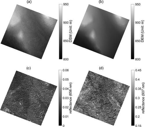
The DSM (Figure 3a) with a spatial resolution of 0.5 m can be obtained from the LiCHy-LiDAR signal. Then, the DEM (Figure 3b) can be extracted based on the DSM through a spatial filtering method, such as the cloth simulation filtering algorithm (Zhang et al. 2016). The CHM can be calculated as the difference between DSM and DEM. Figure 3c-d show the nadir LiCHy-hyperspectral reflectance with a spatial resolution of 1.0 m in the red (656 nm) and NIR (907 nm) bands, respectively. They are used in the case study of section 5 to evaluate the simulated reflectance images.

Figure 3. Estimated KEA DSM from LiCHy-LiDAR measurement (a); estimated KEA DEM from DSM (b); reflectance image of the red band (656 nm) of the KEA obtained by the LiCHy-AISA Eagle II hyperspectral sensor (c); reflectance image of the NIR band (907 nm) of the KEA obtained by the LiCHy-AISA Eagle II hyperspectral sensor (d).

3.2. Multi-spectral multi-angle integrated system: WiDAS

WiDAS is an integrated platform used to simultaneously obtain multi-angle observations from visible and near-infrared (VNIR) and TIR radiance. It was designed by the Institute of Remote Sensing Applications of the Chinese Academy of Sciences and Beijing Normal University in 2008. It is one of the main airborne pieces of equipment in WATER (Li et al. 2009) and HiWATER (Li et al. 2013). The platform integrates two multi-spectral cameras (Condor-MS5) and one TIR camera (FLIR A655sc) to obtain multi-angle radiance in VNIR and TIR bands. The cameras have a forward inclination angle (Table 3) to ensure a maximum viewing zenith angle up to 60°. A very high spatial resolution CCD camera (Phase iXa 645DF) is also included to obtain a 0.4 m spatial resolution base map (Figure 4b) for the other three cameras.

Figure 4. The WiDAS flight tracks (a) and the generated digital orthographic map of the KEA with spatial resolution equal to 0.4 m using Phase iXa 645DF camera (b).

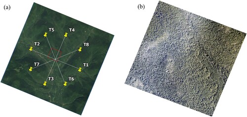
Table 3. Parameters of the WiDAS sensors with a flight height of 2000m.

	iXa 645DF	Condor-MS5	Condor-MS5	FLIR A655sc
Wavelength(nm)	RGB	460,555, 620,685,760	460,555, 620,685,760	7500–14000
Pixels	7760×10328	1360×1024	1360×1024	640×480
FOV	70×87	32×24	32×24	68×54
Oblique Angle	0	14	44	26
Swath (m)	3796	850	850	2038

Multi-angle observations were realized by consecutive observations when the WiDAS sensor passed over an area of interest (Cao et al. 2019). Targets were observed on multiple occasions to form a series of images. The observation angle varied with the relative position between the aircraft and the target. During the FOREST experiment, four planes were observed with flight height equal to 2000 m, including the solar principal plane (i.e. from T1 to T2), cross solar principal plane (i.e. from T3 to T4) and two transition planes (Figure 4a).

3.3. UAV sensors

A six-rotor UAV was selected to mount the sensors (Table 4) to acquire the high spatial resolution images over the KEA. Its battery can support about 30 min of flight with the maximum sensor weight (1 kg). Figure 5a-d shows the flights and the appearances of UAV-CCD, UAV-Hyperspectral and UAV-TIR.

Figure 5. Flights, sensors and artificial geometric targets of UAV observations.

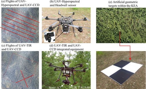
Table 4. Parameters of three UAV sensors.

UAV-CCD	UAV-Hyperspectral	UAV-TIR
Type: Sony A7	Type: Headwall	Type: FLIR TAU640
Wavelength: RGB	Wavelength: 0.38–1.0 μm	Wavelength: 7.5–14 μm
Pixels: 7360×4144	Pixels: 1004×1	Pixels: 640×512
Radiometric resolution: 8 bits	Spectral resolution: 5 nm	Radiometric resolution: 12 bits
Focal length: 35 mm	Focal length: 8 mm	Focal length: 7.5 mm
Weight:0.4 kg	Weight: 0.9 kg	Weight: 0.3 kg
Aim: provide base map	Maximum bands: 325	Pixel size: 17 μm

UAV-CCD was used to provide the base map for the other two sensors because it had a better spatial resolution, which reached 0.05 m at a fight height of 300 m. UAV-CCD had the same six flights (Figure 5a) as UAV-Hyperspectral. Their flight missions were performed successively. The UAV-CCD and UAV-TIR were directly integrated together (Figure 5d) to save flight time because they are much lighter than the hyperspectral sensor (Figure 5b). UAV-TIR had two cross tracks in the southeast region of KEA (Figure 5c). To improve the accuracy of spatial matching, ten artificial geometric targets with an area of 1.5 m × 1.5 m (Figure 5e) were manufactured and placed in the open forest stand within the KEA.

Headwall (Figure 5b) is a linear array push-broom hyperspectral sensor of VNIR. It can obtain a maximum of 325 bands from 380 to 1000 nm. Considering the UAV-Hyperspectral fight height (300 m) and field of view, six parallel tracks (Figure 5a) were implemented to mosaic a hyperspectral reflectance map of the KEA with 0.3 m spatial resolution. The observations were carried out during the stable growth stage of the trees (August 08, 2016). UAV-TIR was aimed to obtain the forest canopy temperature distribution over the KEA. A TIR camera (FLIR TAU640) was mounted with a CCD camera (Figure 5d). The view angle of the TIR camera is 26° forward as FLIR A655sc of WiDAS. Two flights with heights of 200 and 300 m were carried out on August 15, 2016. To obtain the temperature distribution over the KEA as soon as possible and reduce as much as possible the impact of time on the thermal state, only two cross tracks for each flight covering 500 m × 500 m (Figure 5c) were implemented under the limitation of the battery of the UAV.

4. Ground observation: design and results

4.1. Sampling strategy over heterogeneous land surfaces

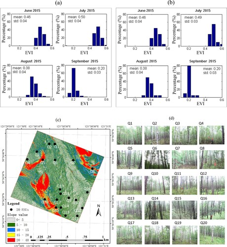
Twenty 30 m×30 m ESUs were established in the KEA according to the optimal Sampling strategy based on the Multi-temporal Prior knowledge (SMP) (Zeng et al. 2015). The SMP approach employed multi-temporal enhanced vegetation index (EVI) maps as a priori knowledge, minimized the multi-temporal bias of the EVI frequency histogram between the ESUs (Figure 6b) and the entire KEA (Figure 6a), and maximized the nearest-neighbor index to ensure that the ESUs achieved good spatial representativeness. The spatial distribution of 20 ESUs and their lateral photos are shown in Figure 6c and d, respectively. Seventeen ESUs are mixed stand with pines and birches while Q9, Q11 and Q12 only consisted of pines (Figure 6d).

Figure 6. EVI histogram of the entire KEA (a) and twenty ESUs (b) in the growth stage of 2015, spatial locations (c) and the lateral photos (d) of twenty ESUs.

4.2. Structural parameters measurements

4.2.1. Height, DBH, crown size and leaf size measurements

The DBH of all trees with DBH > 0.05 m were measured using a tape. Then, the tree height, first branch height and crown size were measured by stratified sampling of the DBH value (including six classes: 0.05∼0.10 m, 0.10∼0.15 m, 0.15∼0.20 m, 0.20∼0.25 m, 0.25∼0.30 m and >0.30 m). The crown size was measured by tapes, and the tree height and first branch height were measured by laser rangefinder (Trupulse-TM2000 and Impulse).

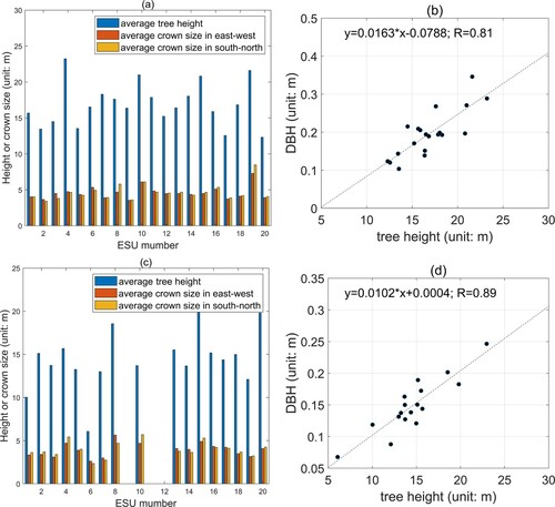
Figure 7 shows the measured average tree heights and average crown sizes and the scatter plot between tree height and DBH. Q9, Q11 and Q12 only contained pines, therefore, they do not have values in Figure 7c. Pines were overall higher than birches (Figure 7a and c). Both tree species show a good positive correlation between tree height and DBH, with R over 0.80 (Figure 7b and d). These structural parameters were used to calibrate the allometric scaling and resource limitation (ASRL) model for predicting the maximum tree height of Great Khingan Mountain (Zhang et al., 2019b).

Figure 7. Average height and crown size of pine (a); the scatter plot between the tree height and DBH of pine (b); average height and crown size of birch (c); and the scatter plot between the tree height and DBH of birch (d).

In addition, the average leaf size of white birch was scanned and measured using Li-3000. Three trees were selected as the samples for each ESU, ten leaves below and up to ten meters of a tree were collected for a total of 60 birch leaves harvested in each stand. The mean leaf area of all ESUs was 22.6 cm².

4.2.2. PAI, LAI, ALIA, FVC and CI measurements

Forest LAI is a key characteristic controlling mass and energy exchanges between the forest and the environment. It is can be obtained based on the PAI and woody-to-total area ratio (α) measurements (i.e. LAI = PAI × (1-α)). It is important for the 3D forest scene reconstruction and forward BRDF/DBT simulation. In addition to three traditional professional measuring instruments (Hemiview, LAI2000, TRAC), two smartphone-based methods (LAISmart (Qu et al. 2016) with the view zenith angle at 0°; and PocketLAI (Confalonieri et al. 2013) with the view zenith angle at 57.5°) were used to measure forest LAI. FVC, measured by Nikon D3000 camera, is also an indicator of LAI. The TRAC can output the CI values as a ratio to convert the effective LAI (LAI_e) to true LAI (LAI_t). The ALIA can be calculated simultaneously with LAI for Hemiview and LAI-2000 measurements, although the ALIA estimation is under the assumption of randomly distributed leaves and there might be some uncertainty when it is used in forests (Yan et al. 2019).

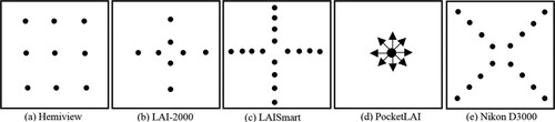
Hemiview, LAI-2000, LAISmart, PocketLAI and Nikon D3000 camera were measured in cloudy weather conditions whereas the TRAC was carried out in sunny conditions, with different sampling approaches (Figure 8). There are nine uniformly distributed points of Hemiview observations with each ESU. The LAI-2000 was held by an operator walking along an east–west route and a north–south route, obtaining four pieces of canopy transmittance data in each line, thus there were 8 LAI-2000 points in one ESU. LAI-2000 contains two sensors: one was vertically placed in the open space outside the forest to measure the total downward sky radiance and the other sensor measured within the ESU with a 180° lens cap. LAISmart obtained eight observations at approximately regular intervals along an east–west route and a north–south route as LAI-2000, giving 16 observed values for one ESU. For PocketLAI, photographed along eight azimuths at 45 intervals, obtaining eight observed values with the zenith angle of the smartphone at 57.5°. Nikon D3000 obtained 16 pictures at the two diagonal lines of each ESU for the FVC observation. However, the TRAC was measured in the cross solar principal plane with a stable walking speed less than 0.3 m/s.

Figure 8. Different sampling approaches for Hemiview (a), LAI-2000 (b), LAISmart (c), PocketLAI (d), and Nikon D3000 camera (e).

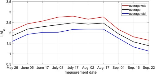
The FOREST experiment was carried out intensively from August 02–17. This period was stable according to the LAISmart series results (Figure 9). LAISmart was carried out for all ESUs every two weeks from 26 May to 22 September, 2016. Qu et al. (2017) compared the extracted LAIs of LAISmart and PocketLAI taking the results of LAI2000 as the reference. They found that the method with the smartphone oriented vertically upwards (i.e. LAISmart) always produced better consistency in magnitude with LAI2000, and PocketLAI underestimated the conifer LAI due to the overestimation of the gap fraction.

Figure 9. Time series of LAI of all ESUs measured by LAISmart.

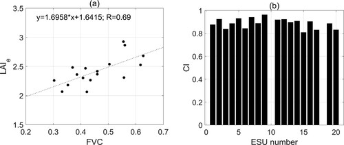
The FVC was extracted using an automatic thresholding method (Liu et al. 2012). It is ranged from 0.29–0.62 and had a good correlation (R=0.69) with LAISmart measured LAI_e (see Figure 10a). The CI extracted from TRAC ranged from 0.80–0.96 with an average equal to 0.89 for the 18 ESUs (no effective observation for Q10 and Q18, see Figure 10b). In addition, the terrestrial LiDAR was performed in 11 ESUs, including Q2-Q5, Q9-Q11, Q15, Q17–18 and Q20. It can provide detailed structure information for the ESUs as an important component of the ground measurements.

Figure 10. Scatter plot between the in situ-measured FVC and the measured LAIe using LAIsmart in Aug. 02, 2016 (a); and the measured CI using TRAC in ESUs in Aug. 08, 2016 (b).

4.3. Spectral parameters measurements

4.3.1. Component reflectance and transmittance

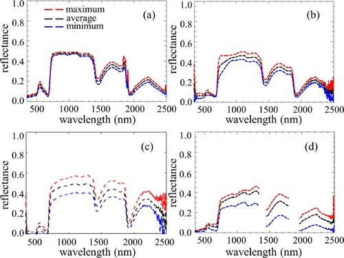
The reflectance of the pine and birch leaves were measured by an integrating sphere in the lab (Figure 11a-b). The pine needles were pasted tightly into one layer in the measurements by the integrating sphere, which was different from the measurements of the broad leaves of birches. In addition, the transmittance of white birch leaves (Figure 11c), the reflectance of the background (Figure 11d) and bark of the pine and birch were measured by ASD in the field at noon time on sunny days.

Figure 11. The measured reflectance of pine leaves (a), reflectance of white birch leaves (b), transmittance of white birch leaves (c) and reflectance of background (d). The red, blue, and black line represent the maximum, minimum and average value of the reflectance spectra, respectively.

4.3.2. Component temperature variation

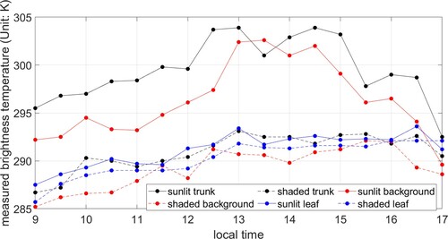
The temperature of sunlit/shaded leaf, sunlit/shaded background and sunlit/shaded trunk were measured using the portable TIR instrument FLIR T440 (Figure 12). These six component temperatures of Q9 were measured every half hour from 9:00–17:00 on August 19, 2016. The temperature difference between sunlit and shaded leaves was less than 3 K. However, the sunlit background (trunk) was 11.7 K (12.1 K) warmer than the related shaded component at local 13:00 (12:30). This measurement has been used to drive a newly developed forest canopy geometric optical DBT model with the ability to simulate the contribution of trunks (Bian et al. 2021).

Figure 12. Daytime temperature variation of six components measured on August 19, 2016.

5. A case study based on the FOREST dataset

There were three objectives in the FOREST experiment, including large 3D scene reconstruction, analytical forward BRDF/DBT model validation and forest parameter estimation method validation. Here, we evaluate the first objective using the FOREST dataset and the 3D radiative transfer model LESS (Qi et al. 2019). 3D canopy radiative transfer models can accurately simulate canopy reflectance and brightness temperature based on detailed and complex 3D structures. However, their accuracies are always limited by the reliability of 3D scenes, such as the precision of structural and spectral parameters. Therefore, the uncertainty of 3D model simulated BRDF/DBT can be used as an important indicator of the accuracy of the reconstructed 3D scene.

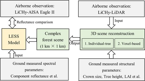
In this section, we first reconstructed two 1 km ×1 km 3D scenes for the KEA based on the airborne LiCHy-LiDAR measurement (8.8 points/m²) and ground-measured structural parameters. One scene was built using the individual-tree approach and the other one was generated using the voxel-based approach. Then, the ground-measured component reflectance and transmittance parameters were input into the LESS model for canopy reflectance simulation. Finally, the LiCHy-Hyperspectral sensor-measured canopy reflectance in the red and NIR bands (see Figure 3c-d) was used to validate the LESS-simulated results. The correlation between LESS-simulated reflectance and LiCHy-measured reflectance can be used to evaluate the quality of the FOREST dataset. The flowchart of this case study is given in Figure 13.

Figure 13. Flowchart of a case study of large-scale canopy reflectance simulation using LESS for the evaluation of the reconstructed 3D scenes based on FOREST dataset.

5.1. Large 3D scene reconstruction

A widely-used approach to build 3D forest scenes is reconstructing the detailed structures of individual trees and populating these tree models in a virtual forest scene according to the actual tree positions and crown diameters extracted from airborne LiDAR data (i.e. individual-tree approach). Another approach is to divide the space into 3D regular voxels and calculates the plant area volume density (PAVD) for each voxel (i.e. voxel-based approach). The latter approach is more efficient than the individual-tree approach since it avoids the detection of individual trees and the detailed description of the tree morphology. Both approaches were considered in this case study as illustrated in Figure 14a, c, e, and b, d, f, respectively.

Figure 14. Estimated KEA CHM with spatial resolution of 0.5 m (i.e. DSM-DEM) (a) and KEA PAI with spatial resolution of 2 m from LiCHy-LiDAR (b); pine trees with heights of 7.2, 12.68, 18.42 m, respectively, and birch trees with heights of 13.2, 17.8 and 24.9 m, respectively (c); three typical cells with different amounts of leaves with leaf area volume density (LAVD) of 0.5, 1.5 and 2.5, respectively (d); reconstructed 3D scene using individual-tree approach (e); reconstructed 3D scene using voxel-based approach (f).

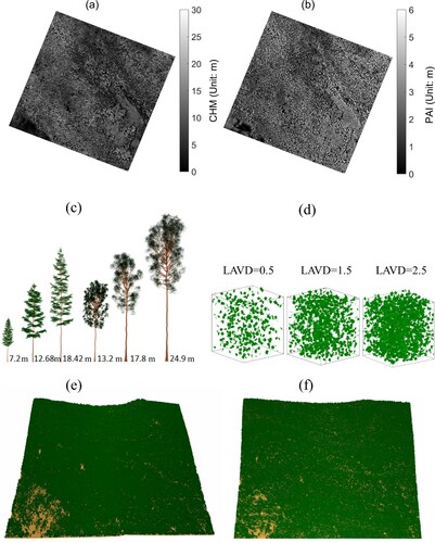
The CHM (Figure 14a) was equal to the difference between the DSM and DEM (Figure 3a-b). The locations and crown sizes of each detected tree object were extracted from the CHM map using a watershed-based segmentation tool provided by LESS. Six individual trees (three pine trees and three birch trees in Figure 14c), whose heights and crown diameters were from in situ measurements, were generated by using the Onyx Tree software (www.onyxtree.com) for the individual-tree approach. The 3D landscape was constructed by instantiating these trees in different locations. The tree object which has the most similar tree height and tree crown diameter of the detected tree, quantified by a single tree similarity factor, was chosen and placed on the DEM to save memory use (Qi et al. 2017). Figure 14e shows the visualization of the final reconstructed scene using individual-tree approach. In total, 135,818 trees were planted in this area.

For the voxel-based approach, the total transmittance of each voxel was estimated by the total transmitted LiDAR energy. Then, the 2D PAI in a grid resolution of 2 m was determined by applying the Beer law under the assumption of spherical leaf angle distribution (Figure 14b). To determine the vertical distribution of plant material, we divided the 2-m column into 2×2×2 m voxels starting from the ground using the method proposed by Schneider et al. (2014): total PAVD was distributed into each voxel by using the proportion of points to the total points in this column. Fifty basic voxels with different leave area volume density (LAVD) ranged from 0.1–5 with a step of 0.1. Figure 14d shows three typical voxels with LAVD of 0.5, 1.5 and 2.5, respectively. Each voxel was filled with randomly distributed triangles with their leaf normal directions following the spherical distribution. Then, these basic voxels were instantiated and populated into the 3D scene according to the retrieved 3D LAVD distribution. Figure 14f illustrates the reconstructed 3D scene that was composed of many voxels.

5.2. Reflectance simulation using LESS model

The LESS simulation was carried out with the same spatial resolution (1 m) as LiCHy-Hyperspectral and with two typical bands for vegetated canopy (red and NIR). The component reflectance and transmittance spectra in Figure 11 were used to drive the LESS simulations. Specifically, the input leaf reflectance, leaf transmittance and background reflectance were equal to 0.07, 0.07 and 0.04 for the red band (656 nm), equal to 0.43, 0.43, and 0.25 for the NIR band (907 nm). The spectral parameters of the large scene were the same for all pixels, which may lead to some uncertainty in the simulated canopy reflectance.

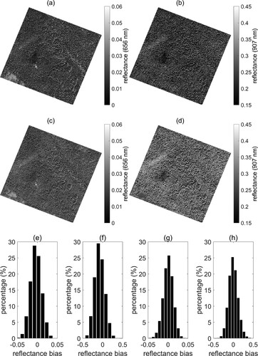
The sun zenith and azimuth angles (42.3°, 163.0°) were calculated by the Sun Position Calculator tool of LESS based on the flight date, time, and geographical position of KEA. The sensor was set to orthographic projection with view zenith angle equal to zero. This simulation took around 50 min on a laptop with 16 GB memory and 8 cores. Four reflectance images were simulated for comparison with the LiCHy-Hyperspectral measured image. Figure 15a-b illustrates the LESS simulated results using the individual-tree approach while Figure 15c-d shows the results using the voxel-based approach. It can be found that the results of the voxel-based approach were brighter than the corresponding image of the individual-tree approach and closer to the LiCHy-Hyperspectral measured images. However, the simulated images are much more homogeneous than the airborne measured images. We can obtain the reflectance difference between the measured and simulated results in the two bands. Figure 15e-h show the reflectance bias histograms for Figure 15a-d, respectively. It can be found that the simulated results of the individual-tree approach were overall underestimated whereas the histogram of the reflectance bias of the voxel-based approach simulated results was close to the normal distribution.

Figure 15. LESS simulated image of the red band (a) and the NIR band (b) using the individual-tree approach; LESS simulated image of the red band (c) and the NIR band (d) using the voxel-based approach; histogram of the reflectance bias of the LESS-simulated image of the red band (e) and the NIR band (f) using the individual-tree approach; histogram of the reflectance bias of the LESS-simulated image of the red band (g) and the NIR band (h) using the voxel-based approach.

5.3. Reflectance validation using LiCHy-Hyperspectral image

Figure 16 shows the scatter plot of the LiCHy images and LESS simulated images in both red and NIR bands. For better evaluation of the simulated reflectance, the images in Figure 15 and Figure 3c-d were resized to 30-m spatial resolution. Therefore, each sub-image contains 1089 points (i.e. 33 lines × 33 samples).

Figure 16. Scatter plot of the LiCHy image and LESS simulated image at 656 nm using the individual-tree approach (a); scatter plot of the LiCHy image and LESS simulated image at 907 nm using the individual-tree approach (b); scatter plot of the LiCHy image and LESS simulated image at 656 nm using the voxel-based approach (c); scatter plot of the LiCHy image and LESS simulated image at 907 nm in the voxel-based approach (d).

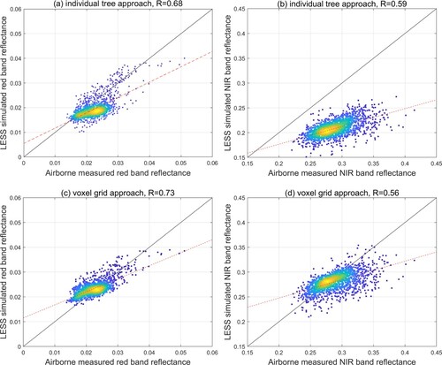
The simulated reflectance images using the individual-tree approach were underestimated, as shown in Figure 16a-b. The image in the red (NIR) band has a R of 0.68 (0.59). The reasons for the reflectance bias include: (1) the mean optical properties of 20 ESUs were applied to all elements in the landscape. Therefore, it cannot clearly reflect the heterogeneity of the scene optical properties, which leads to the actual images being more heterogeneous than the simulated images; (2) the inconsistency of PAI for each pixel is due to the trees within the mock-up are selected only by tree height and crown diameter. The PAI of each tree model is fixed in the 3D scene reconstruction. Overall, only six tree objects were used in this simulation, and they do not represent all the trees in the KEA, especially the PAI variation at fine scales, although the images were resized into 30 m. However, the simulated accuracies are acceptable compared with the results (R=0.54 for the red band and R=0.58 for the NIR band) of Schneider et al. (2014).

Figure 16c-d show that the LESS simulated images using the voxel-based approach are closer to the actual airborne images than Figure 16a-b. The R of the simulated reflectance image is equal to 0.73 for the red and 0.56 for the NIR band, which are close to the results (R=0.62 for the red band and R=0.69 for the NIR band) of Schneider et al. (2014). The differences between the LESS-simulated image and LiCHy-Hyperspectral image can be explained by two reasons: (1) the same optical properties (i.e. leaf reflectance and transmittance, background reflectance) were assigned to all elements in the large scene. This simplifying hypothesis does not match the real forest, which usually has spatially varying optical properties; (2) the trunks and branches are not specially handled, since they are considered as leaves and are involved in the LAVD of voxels.

6. Summary

This paper introduced the objectives and airborne/ground observations of fine-scale optical remote sensing experiment of mixed stand over complex terrain in the Genhe Reserve Area. The objectives included a large 3D scene reconstruction, the forward model validation and the forest parameter retrieval method validation. The LiCHy and WiDAS were mounted on a Yun-5 aircraft to obtain optical signals of the land surface. The UAV was adopted to acquire high spatial resolution hyperspectral images, thermal infrared images, and related CCD images. Within the KEA, twenty ESUs were established considering the representation of the spatial and temporal features of the KEA. Both structural (i.e. tree height, DBH, crown size, leaf size, PAI, LAI, ALIA, FVC and CI) and spectral (i.e. component reflectance, transmittance, and temperature) parameters were measured for each ESU.

The first objective was evaluated in detail using the FOREST dataset in this study. Two large (1 km×1 km) 3D scenes were reconstructed using an individual-tree approach and voxel-based approach, respectively, based on the observations of airborne LiCHy-LiDAR and ground measured structural parameters. The ground-measured spectral parameters, LESS-calculated solar and viewing angles were adopted to drive the LESS model for simulating the canopy reflectance. The good consistency between the LESS outputs and the airborne LiCHy-Hyperspectral images for the red band (R=0.68–0.73) and for the NIR band (R=0.56–0.59) shows the high quality of the experiment. The LESS-simulated reflectance was limited by the spatial representativeness of input component reflectance and transmittance and the accuracy of reconstructed large-scale canopy architecture. More work needs to be done to further improve the reliability of the reconstructed large 3D scene. The FOREST dataset can benefit forest research communities for validating analytical forward forest canopy models and evaluating forest parameter retrieval methods (i.e. the second and third objectives of this experiment).

Glossary

Table

FOREST	Fine scale Optical Remote sensing Experiment of mixed Stand over complex Terrain	KEA	Key Experiment Area
ESU	Elementary Sampling Unit	LESS	LargE-Scale remote sensing data and image Simulation framework over heterogeneous 3D scenes
RAMI	RAdiative transfer Model Intercomparison	BOREAS	Boreal Ecosystem-Atmosphere Study
COMPLICATE	Complicate Observations and Multi-Parameter Land Information Constructions on Allied Telemetry Experiment	LiDAR	Light Detection And Ranging
CCD	Charge Coupled Device	DBH	Diameter at Breast Height
PAI	plant area index	LAI	Leaf Area Index
ALIA	Average Leaf Inclination Angle	FVC	Fraction of Vegetation Cover
CI	Clumping Index	LiCHy	LiDAR-CCD-Hyperspectral integrated mission
WiDAS	Wide-angle Infrared Dual-mode line/area Array Scanner	UAV	Unmanned Aerial Vehicle
WATER	Watershed Allied Telemetry Experimental Research	HiWATER	Heihe Watershed Allied Telemetry Experimental Research
BRDF	Bi-directional Reflectance Distribution Function	DBT	Directional Brightness Temperature
TRAC	Tracing Radiation and Architecture of Canopies	DSM	Digital Surface Model
DEM	Digital Elevation Model	CHM	Canopy Height Model
VNIR	Visible and Near-Infrared	TIR	Thermal infrared
EVI	Enhanced Vegetation Index	ASRL	Allometric Scaling and Resource Limitation
PAVD	Plant Area Volume Density	LAVD	Leaf Area Volume Density
NIR	Near-Infrared

Geolocation information

The study area in this paper is Northeast of Inner Mongolia, China.

Acknowledgments

We thank the participants of the experiment, including scientists, engineers, pilots and students. They include Yong Pang, Qingwang Liu, Wen Jia for LiCHy measurement, Junyong Fang, Xue Liu, Baochang Gong for the WiDAS and UAV measurements, Yelu Zeng, Yonghua Qu, Shaojie Zhao for ESU selection, Xin Tian, Yuli Shi for tree Height measurement, Shuai Gao for leaf size measurement, Shihua Li and Wenjie Fan for Hemiview measurement, Yonghua Qu for LAI2000, LAISmart, PocketLAI measurements, Dashuai Guo, Zhan Gao and Jinghui Luo for the FVC and TRAC measurements, Yelu Zeng and Yadong Dong for the leaf/soil reflectance measurement, Zunjian Bian for the component temperature measurement.

Data availability statement

The data that support the findings of this study are available from the first author ([email protected]) or the corresponding author ([email protected]), upon reasonable request. Part of the dataset can be downloaded from the website of the National Tibetan Plateau Data Center of China (http:// data.tpdc.ac.cn/en/)

Disclosure statement

No potential conflict of interest was reported by the author(s).

Additional information

Funding

This work was supported in part by the National Basic Research Program of China (2013CB733400), in part by the Natural Science Foundation of China (41930111 and 41871258); in part by the Youth Innovation Promotion Association CAS under Grant 2020127; in part by the ‘Future Star’ Talent Plan of the Aerospace Information Research Institute of Chinese Academy of Sciences under Grant Y920570Z1F.

References

- Bian, Z., B. Cao, H. Li, Y. Du, W. Fan, Q. Xiao, and Q. Liu. 2021. “The Effects of Tree Trunks on Directional Emissivity and Brightness Temperatures of a Leaf-off Forest Using a Geometric Optical Model.” IEEE Transactions on Geoscience and Remote Sensing 59: 5370–5386.
- Bian, Z., B. Cao, H. Li, Y. Du, J.-P. Lagouarde, Q. Xiao, and Q. Liu. 2018. “An Analytical Four-Component Directional Brightness Temperature Model for Crop and Forest Canopies.” Remote Sensing of Environment 209: 731–746. doi:https://doi.org/10.1016/j.rse.2018.03.010.
- Bian, Z., Q. Xiao, B. Cao, Y. Du, H. Li, H. Wang, Q. Liu, and Q. Liu. 2016. “Retrieval of Leaf, Sunlit Soil, and Shaded Soil Component Temperatures Using Airborne Thermal Infrared Multiangle Observations.” IEEE Transactions on Geoscience and Remote Sensing 54: 4660–4671. doi:https://doi.org/10.1109/TGRS.2016.2547961.
- Cao, B., Y. Du, J. Li, H. Li, L. Li, Y. Zhang, J. Zou, and Q. Liu. 2015. “Comparison of Five Slope Correction Methods for Leaf Area Index Estimation from Hemispherical Photography.” IEEE Geoscience and Remote Sensing Letters 12: 1958–1962. doi:https://doi.org/10.1109/LGRS.2015.2440438.
- Cao, B., M. Guo, W. Fan, X. Xu, J. Peng, H. Ren, Y. Du, et al. 2018. “A New Directional Canopy Emissivity Model Based on Spectral Invariants.” IEEE Transactions on Geoscience and Remote Sensing 56: 1–16..
- Cao, B., Q. Liu, Y. Du, J.-L. Roujean, J.-P. Gastellu-Etchegorry, I. F. Trigo, W. Zhan, et al. 2019. “A Review of Earth Surface Thermal Radiation Directionality Observing and Modeling: Historical Development, Current Status and Perspectives.” Remote Sensing of Environment 232: 111304. doi:https://doi.org/10.1016/j.rse.2019.111304.
- Cao, B., J.-L. Roujean, J.-P. Gastellu-Etchegorry, Q. Liu, Y. Du, J.-P. Lagouarde, H. Huang, et al. 2021. “A General Framework of Kernel-Driven Modeling in the Thermal Infrared Domain.” Remote Sensing of Environment 252: 112157. doi:https://doi.org/10.1016/j.rse.2020.112157.
- Chen, J. M. 2021. “Carbon Neutrality: Toward a Sustainable Future.” The Innovation 2(3), 100127. doi: https://doi.org/10.1016/j.xinn.2021.100127.
- Chen, J. M., and J. Cihlar. 1996. “Retrieving Leaf Area Index of Boreal Conifer Forests Using Landsat TM Images.” Remote Sensing of Environment 55: 153–162. doi:https://doi.org/10.1016/0034-4257(95)00195-6.
- Chmura, D. J., P. D. Anderson, G. T. Howe, C. A. Harrington, J. E. Halofsky, D. L. Peterson, D. C. Shaw, and J. B. St Clair. 2011. “Forest Responses to Climate Change in the Northwestern United States: Ecophysiological Foundations for Adaptive Management.” Forest Ecology and Management 261: 1121–1142. doi:https://doi.org/10.1016/j.foreco.2010.12.040.
- Confalonieri, R., M. Foi, R. Casa, S. Aquaro, E. Tona, M. Peterle, A. Boldini, et al. 2013. “Development of an app for Estimating Leaf Area Index Using a Smartphone. Trueness and Precision Determination and Comparison with Other Indirect Methods.” Computers and Electronics in Agriculture 96: 67–74. doi:https://doi.org/10.1016/j.compag.2013.04.019.
- Fan, W., J. Li, and Q. Liu. 2015. “GOST2: The Improvement of the Canopy Reflectance Model GOST in Separating the Sunlit and Shaded Leaves.” IEEE Journal of Selected Topics in Applied Earth Observations and Remote Sensing 8: 1423–1431. doi:https://doi.org/10.1109/JSTARS.2015.2413994.
- Gastellu-Etchegorry, J. P., N. Lauret, T. G. Yin, L. Landier, A. Kallel, Z. Malenovsky, A. Al Bitar, et al. 2017. “DART: Recent Advances in Remote Sensing Data Modeling With Atmosphere, Polarization, and Chlorophyll Fluorescence.” IEEE Journal of Selected Topics in Applied Earth Observations and Remote Sensing 10: 2640–2649. doi:https://doi.org/10.1109/jstars.2017.2685528.
- Geng, J., J. M. Chen, W. Fan, L. Tu, Q. Tian, R. Yang, Y. Yang, L. Wang, C. Lv, and S. Wu. 2017. “GOFP: A Geometric-Optical Model for Forest Plantations.” IEEE Transactions on Geoscience and Remote Sensing 55: 5230–5241. doi:https://doi.org/10.1109/TGRS.2017.2704079.
- Halldin, S., S. E. Gryning, L. Gottschalk, A. Jochum, L. C. Lundin, and A. A. Van de Griend. 1999. “Energy, Water and Carbon Exchange in a Boreal Forest Landscape - NOPEX Experiences.” Agricultural and Forest Meteorology 98-99: 5–29. doi:https://doi.org/10.1016/s0168-1923(99)00148-3.
- Hao, D., J. Wen, Q. Xiao, S. Wu, X. Lin, D. You, and Y. Tang. 2018. “Modeling Anisotropic Reflectance Over Composite Sloping Terrain.” IEEE Transactions on Geoscience and Remote Sensing 56: 3903–3923. doi:https://doi.org/10.1109/TGRS.2018.2816015.
- Hao, D., J. Wen, Q. Xiao, D. You, and Y. Tang. 2020. “An Improved Topography-Coupled Kernel-Driven Model for Land Surface Anisotropic Reflectance.” IEEE Transactions on Geoscience and Remote Sensing 58: 2833–2847. doi:https://doi.org/10.1109/TGRS.2019.2956705.
- Hu, T., Y. Du, B. Cao, H. Li, Z. Bian, D. Sun, and Q. Liu. 2016. “Estimation of Upward Longwave Radiation from Vegetated Surfaces Considering Thermal Directionality.” IEEE Transactions on Geoscience and Remote Sensing 54: 6644–6658. doi:https://doi.org/10.1109/TGRS.2016.2587695.
- Jiao, Z., C. B. Schaaf, Y. Dong, M. Román, M. J. Hill, J. M. Chen, Z. Wang, et al. 2016. “A Method for Improving Hotspot Directional Signatures in BRDF Models Used for MODIS.” Remote Sensing of Environment 186: 135–151. doi:https://doi.org/10.1016/j.rse.2016.08.007.
- Kuusk, A., J. Kuusk, and M. Lang. 2009. “A Dataset for the Validation of Reflectance Models.” Remote Sensing of Environment 113: 889–892. doi:https://doi.org/10.1016/j.rse.2009.01.005.
- Li, L., J. Chen, X. Mu, W. Li, G. Yan, D. Xie, and W. Zhang. 2020. “Quantifying Understory and Overstory Vegetation Cover Using UAV-Based RGB Imagery in Forest Plantation.” Remote Sensing 12: 298. doi:https://doi.org/10.3390/rs12020298.
- Li, X., G. Cheng, S. Liu, Q. Xiao, M. Ma, R. Jin, T. Che, et al. 2013. “Heihe Watershed Allied Telemetry Experimental Research (HiWATER): Scientific Objectives and Experimental Design.” Bulletin of the American Meteorological Society 94: 1145–1160. doi:https://doi.org/10.1175/BAMS-D-12-00154.1.
- Li, X., X. W. Li, Z. Y. Li, M. G. Ma, J. Wang, Q. Xiao, Q. Liu, et al. 2009. “Watershed Allied Telemetry Experimental Research.” Journal of Geophysical Research 114, D22103. doi: https://doi.org/10.1029/2008JD011590.
- Liu, Y. K., X. H. Mu, H. X. Wang, and G. J. Yan. 2012. “A Novel Method for Extracting Green Fractional Vegetation Cover from Digital Images.” Journal of Vegetation Science 23: 406–418. doi:https://doi.org/10.1111/j.1654-1103.2011.01373.x.
- Ma, B., J. Li, W. Fan, H. Ren, X. Xu, Y. Cui, and J. Peng. 2018. “Application of an LAI Inversion Algorithm Based on the Unified Model of Canopy Bidirectional Reflectance Distribution Function to the Heihe River Basin.” Journal of Geophysical Research: Atmospheres 123: 10,671–10,687..
- Niu, X., B. Wang, and W. J. Wei. 2013. “Chinese Forest Ecosystem Research Network: A Platform for Observing and Studying Sustainable Forestry.” Journal of Food, Agriculture and Environment 11: 1008–1016.
- Peng, J., W. Fan, X. Xu, L. Wang, Q. Liu, J. Li, P. Zhao, et al. 2015. “Estimating Crop Albedo in the Application of a Physical Model Based on the Law of Energy Conservation and Spectral Invariants.” Remote Sensing 7: 15536–15560. doi:https://doi.org/10.3390/rs71115536.
- Pang, Y., Z. Li, H. Ju, H. Lu, W. Jia, L. Si, Y. Guo, et al. 2016. “LiCHy: The CAF's LiDAR, CCD and Hyperspectral Integrated Airborne Observation System.” Remote Sensing 8: 398. doi: https://doi.org/10.3390/rs8050398.
- Qi, J. B., D. H. Xie, D. S. Guo, and G. J. Yan. 2017. “A Large-Scale Emulation System for Realistic Three-Dimensional (3-D) Forest Simulation.” IEEE Journal of Selected Topics in Applied Earth Observations and Remote Sensing 10: 4834–4843. doi:https://doi.org/10.1109/jstars.2017.2714423.
- Qi, J., D. Xie, T. Yin, G. Yan, J.-P. Gastellu-Etchegorry, L. Li, W. Zhang, X. Mu, and L. K. Norford. 2019. “LESS: LargE-Scale Remote Sensing Data and Image Simulation Framework Over Heterogeneous 3D Scenes.” Remote Sensing of Environment 221: 695–706. doi:https://doi.org/10.1016/j.rse.2018.11.036.
- Qu, Y., J. Meng, H. Wan, and Y. Li. 2016. “Preliminary Study on Integrated Wireless Smart Terminals for Leaf Area Index Measurement.” Computers and Electronics in Agriculture 129: 56–65. doi:https://doi.org/10.1016/j.compag.2016.09.011.
- Qu, Y. H., J. Wang, J. L. Song, and J. D. Wang. 2017. “Potential and Limits of Retrieving Conifer Leaf Area Index Using Smartphone-Based Method.” Forests 8 (June): 14. doi:https://doi.org/10.3390/f8060217.
- Schneider, F. D., R. Leiterer, F. Morsdorf, J.-P. Gastellu-Etchegorry, N. Lauret, N. Pfeifer, and M. E. Schaepman. 2014. “Simulating Imaging Spectrometer Data: 3D Forest Modeling Based on LiDAR and in Situ Data.” Remote Sensing of Environment 152: 235–250.
- Sellers, P. J., F. G. Hall, R. D. Kelly, A. Black, D. Baldocchi, J. Berry, M. Ryan, et al. 1997. “BOREAS in 1997: Experiment Overview, Scientific Results, and Future Directions.” Journal of Geophysical Research-Atmospheres 102: 28731–28769. doi:https://doi.org/10.1029/97jd03300.
- Tian, X., Z. Y. Li, E. X. Chen, Q. H. Liu, G. J. Yan, J. D. Wang, Z. Niu, et al. 2015. “The Complicate Observations and Multi-Parameter Land Information Constructions on Allied Telemetry Experiment (COMPLICATE).” PLoS One 10: e0137545..
- Wang, X., H. Huang, P. Gong, C. Liu, C. Li, and W. Li. 2014. “Forest Canopy Height Extraction in Rugged Areas With ICESat/GLAS Data.” IEEE Transactions on Geoscience and Remote Sensing 52: 4650–4657. doi:https://doi.org/10.1109/TGRS.2013.2283272.
- Wei, S., H. Fang, C. B. Schaaf, L. He, and J. M. Chen. 2019. “Global 500 m Clumping Index Product Derived from MODIS BRDF Data (2001–2017).” Remote Sensing of Environment 232: 111296. doi:https://doi.org/10.1016/j.rse.2019.111296.
- Wen, J. G., Q. Liu, Y. Tang, B. C. Dou, D. Q. You, Q. Xiao, Q. H. Liu, and X. W. Li. 2015. “Modeling Land Surface Reflectance Coupled BRDF for HJ-1/CCD Data of Rugged Terrain in Heihe River Basin, China.” IEEE Journal of Selected Topics in Applied Earth Observations and Remote Sensing 8: 1506–1518. doi:https://doi.org/10.1109/jstars.2015.2416254.
- Wen, J., Qiang Liu, Q. Xiao, Qinhuo Liu, D. You, D. Hao, S. Wu, and X. Lin. 2018. “Characterizing Land Surface Anisotropic Reflectance Over Rugged Terrain: A Review of Concepts and Recent Developments.” Remote Sensing 10: 370. doi:https://doi.org/10.3390/rs10030370.
- Widlowski, J. L., C. Mio, M. Disney, J. Adams, I. Andredakis, C. Atzberger, J. Brennan, et al. 2015. “The Fourth Phase of the Radiative Transfer Model Intercomparison (RAMI) Exercise: Actual Canopy Scenarios and Conformity Testing.” Remote Sensing of Environment 169: 418–437. doi:https://doi.org/10.1016/j.rse.2015.08.016.
- Wu, S., J. Wen, X. Lin, D. Hao, D. You, Q. Xiao, Q. Liu, and T. Yin. 2019. “Modeling Discrete Forest Anisotropic Reflectance Over a Sloped Surface With an Extended GOMS and SAIL Model.” IEEE Transactions on Geoscience and Remote Sensing 57: 944–957. doi:https://doi.org/10.1109/TGRS.2018.2863605.
- Xu, X., W. Fan, J. Li, P. Zhao, and G. Chen. 2017. “A Unified Model of Bidirectional Reflectance Distribution Function for the Vegetation Canopy.” Science China Earth Sciences 60: 463–477. doi:https://doi.org/10.1007/s11430-016-5082-6.
- Yan, G., R. Hu, J. Luo, M. Weiss, H. Jiang, X. Mu, D. Xie, and W. Zhang. 2019. “Review of Indirect Optical Measurements of Leaf Area Index: Recent Advances, Challenges, and Perspectives.” Agricultural and Forest Meteorology 265: 390–411. doi:https://doi.org/10.1016/j.agrformet.2018.11.033.
- Yin, G. F., A. N. Li, W. Zhao, H. A. Jin, J. H. Bian, and S. B. A. Wu. 2017. “Modeling Canopy Reflectance Over Sloping Terrain Based on Path Length Correction.” IEEE Transactions on Geoscience and Remote Sensing 55: 4597–4609. doi:https://doi.org/10.1109/tgrs.2017.2694483.
- Zeng, Y., J. Li, Q. Liu, Y. Qu, A. Huete, B. Xu, G. Yin, and J. Zhao. 2015. “An Optimal Sampling Design for Observing and Validating Long-Term Leaf Area Index with Temporal Variations in Spatial Heterogeneities.” Remote Sensing 7 (2): 1300–1319. doi:https://doi.org/10.3390/rs70201300.
- Zhang, D., J. Liu, W. Ni, G. Sun, Z. Zhang, Q. Liu, and Q. Wang. 2019a. “Estimation of Forest Leaf Area Index Using Height and Canopy Cover Information Extracted from Unmanned Aerial Vehicle Stereo Imagery.” IEEE Journal of Selected Topics in Applied Earth Observations and Remote Sensing 12: 471–481. doi:https://doi.org/10.1109/JSTARS.2019.2891519.
- Zhang, W., J. Qi, P. Wan, H. Wang, D. Xie, X. Wang, and G. Yan. 2016. “An Easy-to-Use Airborne LiDAR Data Filtering Method Based on Cloth Simulation.” Remote Sensing 8: 501. doi:https://doi.org/10.3390/rs8060501.
- Zhang, Y., Y. Shi, S. Choi, X. Ni, and R. B. Myneni. 2019b. “Mapping Maximum Tree Height of the Great Khingan Mountain, Inner Mongolia Using the Allometric Scaling and Resource Limitations Model.” Forests 10: 380. doi:https://doi.org/10.3390/f10050380.
- Zhao, T., J. Shi, L. Lv, H. Xu, D. Chen, Q. Cui, T. J. Jackson, et al. 2020. “Soil Moisture Experiment in the Luan River Supporting new Satellite Mission Opportunities.” Remote Sensing of Environment 240: 111680. doi:https://doi.org/10.1016/j.rse.2020.111680.
- Zou, J., Y. Zhuang, F. Chianucci, C. Mai, W. Lin, P. Leng, S. Luo, and B. Yan. 2018. “Comparison of Seven Inversion Models for Estimating Plant and Woody Area Indices of Leaf-on and Leaf-off Forest Canopy Using Explicit 3D Forest Scenes.” Remote Sensing 10: 1297. doi:https://doi.org/10.3390/rs10081297.