Deep neural network ensembles for remote sensing land cover and land use classification

ABSTRACT

With the advancement of satellite technology, a considerable amount of very high-resolution imagery has become available to be used for the Land Cover and Land Use (LCLU) classification task aiming to categorize remotely sensed images based on their semantic content. Recently, Deep Neural Networks (DNNs) have been widely used for different applications in the field of remote sensing and they have profound impacts; however, improvement of the generalizability and robustness of the DNNs needs to be progressed further to achieve higher accuracy for a variety of sensing geometries and categories. We address this problem by deploying three different Deep Neural Network Ensemble (DNNE) methods and creating a comparative analysis for the LCLU classification task. DNNE enables improvement of the performance of DNNs by ensuring the diversity of the models that are combined. Thus, enhances the generalizability of the models and produces more robust and generalizable outcomes for LCLU classification tasks. The experimental results on NWPU-RESISC45 and AID datasets demonstrate that utilizing the aggregated information from multiple DNNs leads to an increase in classification performance, achieves state-of-the-art, and promotes researchers to make use of DNNE.

KEYWORDS:

• Classification
• convolutional neural networks (CNN)
• deep neural network ensembles (DNNE)
• land cover and land use (LCLU)
• remote sensing

1. Introduction

Land cover and land use (LCLU) classification, an active research topic in remote sensing (RS), aims to categorize the given RS image with physical cover and man-made structures based on the image content. LCLU classification has a wide range of real-world applications such as environment monitoring, geospatial object detection, urbanization, and natural disaster analysis (Alganci et al. 2019; Sumbul et al. 2019). World-wide projects supported by NASA and EU e.g. the coordination of information on the environment (CORINE) program, have promoted the adaptation of LCLU tasks significantly (Sertel et al. 2018). The emergence of RS platforms that can capture a wide range of information and an increase in earth observation data volume recently made accessible through globally accessible service delivery platforms has facilitated access to an enormous amount of high-resolution RS images and opened a new era in deep learning-based RS research.

However, the advancement in RS technology comes with many challenges and the main divergence arises from the inherent nature of RS images. That being the case, the RS images differ greatly from natural images since RS images contain more complex patterns and exhibit a different level of complexity due to impacts of internal (detector-based) and external (environmental conditions-based) geometric distortions that occurred during the data collection (Yuan et al. 2020). As a consequence, LCLU classification brings many challenges due to its aforementioned inherent nature of RS images, such as atmospheric and topographic effects, earth curvature, seasonal and time-based changes, random bad pixels (shot noise), line-start/stop problems, line or column striping, and drop-outs during data acquisition. A variety of methods have been proposed for the LCLU classification of satellite images in recent years (Senthilnath et al. 2020; Sertel et al. 2018). These methods disintegrated into three main categories and became distinct by considering the usage of the features from different aspects: human-engineering-based methods, unsupervised feature learning-based methods, and deep feature learning-based methods (Zhu et al. 2017; Xia et al. 2020). The early research of LCLU classification mainly was based on the traditional methods that utilize the hand-crafted features e.g. scale-invariant feature transformation (Lowe 2004) and GIST (Torralba and Oliva 2001). These methods concentrate on the visual interpretation by the image analysts and only involve low-level features, thus, limiting the image’s description. On the other hand, unsupervised learning methods are also adopted to automatically describe the image features without any label information (Cheng et al. 2020), e.g. k-means clustering and autoencoders (Hinton and Salakhutdinov 2006). As a result, these methods seemed to be more utilitarian than visual interpretation-based methods due to the ability to extract the features directly from the image. Nonetheless, these unsupervised learning techniques cannot fully benefit from image class features (Cheng et al. 2020).

Moreover, labeling is needed at the last stage of the unsupervised classification while creating information classes or thematic maps. Several types of research have been conducted in various different domains with outstanding results after the rise of deep learning in computer vision. Especially in 2012, ImageNet large-scale visual recognition challenge (Jia et al. 2009) winner AlexNet (Krizhevsky, Sutskever, and Hinton 2012) architecture became the foundation of spaciously record-breaking results in many fields. After this breakthrough, series of more sophisticated deep CNNs were developed. They progressed the results even further (e.g. ResNet (He et al. 2016) and Inception (Szegedy et al. 2016)) by extracting more discriminative features compared to low-level features. DL models can extract robust, attributive, and high-level features from images and implicitly approximate the sophisticated nonlinear connection between environmental parameters by under multi-layer learning (Lecun, Bengio, and Hinton 2015). DL models have outperformed traditional methods with a noticeable advancement in the many fields of remote sensing such as geospatial object detection, scene understanding, and semantic segmentation (Zhao et al. 2019; Shakya, Biswas, and Pal 2021; Xia et al. 2020) Deploying deep neural networks for remote sensing LCLU classification task is no exception. Notably, in Liu et al. (2019), the authors deployed siamese convolutional neural networks (CNN) with customized euclidean regularization term to boost the model’s performance and achieve 92.11% overall accuracy on the NWPU-RESISC45 dataset. In Zhang, Tang, and Zhao (2019), authors proposed a method, namely CNN-CapsNet, that harnesses from both CNN and capsule networks to capture the hierarchical structure of image content more effectively with intent to make full use of CNN along with CapsNet, achieves 92.6% overall accuracy on NWPU-RESISC45 and 96.85% on AID by removing fully connected layers from CNN and adding capsule networks. In (Yu, Li, and Liu 2020), a GAN-based and attention module integrated approach is proposed to increase the representation power of the customized discriminator for unsupervised LCLU classification. It achieves 77.99% overall accuracy on the NWPU-RESISC45 dataset and 78.95% overall accuracy on the AID dataset. Many researchers increasingly utilize ensembles of multiple deep neural networks for LCLU classification tasks and produce results comparable to state-of-the-art methods. The use of ensemble learning methods not only improves the accuracy, but also enhances the generalization ability of the classifier as stated by a collection of studies (Dietterich 2000; Drucker, Schapire, and Simard 1993; Granitto, Verdes, and Ceccatto 2005; Huggins, Campbell, and Broderick 2016). This characteristic of DNNE could be explained by the hypothesis that combining several learners results in restricting the solution space and producing more generalizable results.

In Minetto, Segundo, and Sarkar (2019), authors proposed a method, namely Hydra, an ensemble of CNN for geospatial land classification in which they first created a coarsely optimized CNN as a starting point and then fine-tuned the weights multiple times by adopting methods to increase the diversity between individual ensemble models towards prompting convergence to different endpoints to form a DNNE. In this paper, the authors further compared the performance of Hydra, along with classifiers based on hand-crafted features such as LBP, GIST, and Color histograms; unsupervised feature learning methods such as BoVW and LLC; DNN architectures such as DenseNet and ResNet. As a result, none of the methods except the DNNs achieves more than 45% accuracy while DenseNet and ResNet achieve 93.3% and 91% accuracy values, respectively, Hydra achieves 94.51% accuracy on NWPU-RESISC45 dataset. Moreover, several winners and top performers on the ImageNet challenge are ensembles of neural networks (Lee et al. 2015). An ensemble approach, MotherNet, was proposed to capture the structural similarity between a cluster of networks by reducing the number of epochs for training. This has resulted in rapid training and higher accuracy. They compared the results of MotherNets to Knowledge Distillation (KD), Snapshot Ensembles (SE), and TreeNets (TN) by evaluating the training cost and the resulting accuracy of an ensemble. The lowest test error rate was obtained for MotherNets. Utilizing DNNE methods enhances the representational power of DNNs and enables to the improvement of the generalization ability (Wasay et al. 2018).

Overall, the main contributions of this research are summarized as follows. First, we have created a benchmark on DNNE by deploying three DNNE methods and addressing their intrinsic superiorities in the context of RS LCLU classification: SE (Huang et al. 2017), Stochastic Weight Averaging (SWA) (Izmailov et al. 2018), and Fast Geometric Ensemble (FGE) (Garipov et al. 2018). We conducted a comparative analysis of recent DNNE methods on the LCLU classification task and pointed to the best-performing DNNE approach. This benchmark study could be beneficial for the ensemble-based deep LCLU classifications with the same data set and transfer learning of DNNE approaches for different data sets. Second, we analyzed the generalizability and robustness of the models for the LCLU classification task by comparing them with the state-of-the-art performance on two challenging large-scale remote sensing datasets, namely AID and NWPU-RESISC45. Third, we showed that DNNE helps to improve the overall accuracy, precision, recall, user accuracy, and producer accuracy up to three percent compared to plain DNN with no ensemble methods involved and further improve the class-wise accuracies.

2. Deep neural network ensembles

The ensembles of classifiers are constituted by aggregating multiple classifiers trained to perform the same task and this way of combining leads to expectantly more precise predictions (Lee et al. 2015). Diversity of classifiers is a very important concept and criterion in ensemble learning. The main objective of ensemble methods is to ensure the diversity of the combined models (Bishop 2006). Relying on a single model has limitations and might be prone to errors due to the single-classifiers’ one-shot nature. Therefore, utilizing information from multiple learners can be advantageous (Wasay et al. 2018). Thus, by aggregating the models that are designed to be diverse, ensemble learners can outperform each of those models when they are trained independently. In the end, it is most likely to boost the performance of each of these weak learners if they were to be used separately (Lee et al. 2015).

3. Method

3.1. Snapshot ensemble

In Snapshot Ensemble (SE), the model converges several local minimums along its optimization path and records them. A cosine annealing learning rate schedule is used to force the model to converge to local minimums along its optimization path (Huang et al. 2017). Thus, the model is addressed through local minimums (or near to them) in the weight space. According to configurations in this paper, in every kth epoch, the learning peaks. As a result, the model forges to converge to a local minimum. Then, the saved snapshots from the training process were combined by averaging.

3.2. Fast geometric ensemble

Fast Geometric Ensemble (FGE) and SE rely on similar foundations; both manipulate the learning rate over epoch. The dissimilarity is that FGE uses a linear piecewise cyclical learning rate. The novelty in this method is discovering an existing connected path between local minima where loss stays relatively low (Garipov et al. 2018). FGE profits these paths by taking snapshots along the way and creating an ensemble out of the saved snapshots. Ultimately, this way of ensemble constitutes models that are diverse enough to aggregate. This method is as expensive as SE in terms of computation since it requires the saved models to be stored before the final classification.

3.3. Stochastic weight averaging

The Stochastic Weight Averaging (SWA) method simply averages the points located in the low loss region of the weight space (Izmailov et al. 2018). This action depends on the prior knowledge of local minimums accumulating at the border of the areas on the loss surface, and in these areas, the loss value is considered low. SWA takes the average of these points and produces a more generalizable outcome. The method raised in the paper produces two models; the first model stores the running average of the model weights, and the second model traverses the weight space and explores by using a learning rate schedule such as cyclical learning rate. Then, the second model’s weights are used for updating the first model. This approach produces one model and requires storing only two models in memory during the training phase. Hence, enables to improve the generalization performance at no additional cost compared to individual training of the learning rate over the epoch. The dissimilarity is that FGE uses a linear piecewise cyclical learning rate and the novelty in this method is the discovery of an existing connected path between local minima where loss stays relatively low (Garipov et al. 2018). FGE profits these paths by taking snapshots along the way and creating an ensemble out of the saved snapshots. Ultimately, this way of ensemble constitutes models that are diverse enough to aggregate. This method is as expensive as SE in terms of computation since it requires the saved models to be stored before the final classification.

4. Experimental setup

This section introduces the datasets, experimental setup, evaluation assessment metrics, and experiment results.

4.1. Datasets and evaluation metrics

Since the deep learning approaches are data-driven concepts, preparing a proper dataset has a crucial impact on the outcome of the task. Hence, an extensive training set and a high number of annotated images are required to learn effective models (Cheng et al. 2020). In this work, instead of using datasets that are already saturated performance-wise (UC-Merced), large-scale publicly available remote sensing datasets namely NWPU-RESISC45 and AID were used due to their abundance in terms of the number of LCLU classes and images (Cheng et al. 2020). The summarization of the datasets is listed in Table 1. Both data sets were generated from GoogleEarth images covering mostly high-resolution satellite images. NWPU-RESISC45 has 45 different LCLU classes and AID has 30 different classes; both datasets provide a wide range of different land categories that could be used as a reference for various remote sensing applications.

Table 1. Details of the datasets.

Datasets	Spatial resolution	Image size	Classes	Total images	RS source
NWPU-RESISC45	0.2–30 m	256 × 256	45	31.500	Google Earth
AID	0.5–8 m	600 × 600	30	10.000	Google Earth

It is crucial to evaluate the quality of the classification results to understand the capability of the used classification approach on extracting semantic information. The results of the conducted experiments were assessed by analyzing the well-known and widely used metrics: Confusion matrix, user accuracy (UA), producer accuracy (PA), overall accuracy, precision, recall, and F1 score. The confusion matrix is a table-wise representation of the actual/reference classes and corresponding algorithm predictions which enables quantitatively assessing the classification performance. PA values provide valuable insights on the algorithm performance by indicating the number of occasions in which the actual land cover/use class is identified on the resulting classification as the same class. UA values indicate the number of occasions in which the classified land cover/use class truly represents that class on the ground (Şimşek and Sertel 2018). F1 score simply calculates the harmonic mean of the precision and recall scores.

4.2. Implementation details

We used ImageNet pre-trained weights for all of the conducted experiments to speed up the training process and harness the feature extraction power of a model that trained on 1.2 million images. Also, the same portion of training and test sets similar to current published literature were used in each experiment to create coherent and comparable experiment results. We applied two commonly used split ratios for each dataset to ensure comparativeness and evaluate the experiments precisely (Cheng et al. 2020). For the NWPU-RESISC45 dataset, the ratio of the training sample is 20%; whereas this ratio is 50% for the AID dataset. For all experiments, a categorical cross-entropy loss function was used. As an architecture, pre-trained InceptionResNetV3 was selected except for the FGE in which VGG16 was used. All training stages were limited to 100 epochs, cyclic cosine annealing learning rate schedule varying between 10⁻² and 10⁻⁴ with 5 snapshots was adopted for the SE, the cyclic learning rate was used for the SWA with the 10⁻² and 10⁻³ limit values and frequency of weight averaging was set to 2, learning rates for remaining experiments were set to 10⁻⁴. We utilized the SGD optimizer with the momentum value of 0.9, and the DNNs weights were initialized using the He initialization technique. Since the architectures used in this research are heavy in terms of parameters and consist of many layers, there is a high probability that the network overfits. Therefore, data augmentation and regularization techniques were employed to overcome this problem. Data augmentation was applied to artificially increase the dataset size by implementing different image transformation approaches to make the DNN more robust to real-life challenges during the inference. Rotation, horizontal and vertical flip, zoom, brightness adjustment, RGB shift, and shearing were used during the augmentation. Regularization methods such as weight regularization and dropout, where the first helps to penalize large weight values and seeks for the simple possible solution (parameters) exist in the loss surface by convexifying the loss surface, and the latter randomly deactivate the neurons (along with their corresponding connections) from the neural network during training were also employed.

4.3. Experimental results and discussions

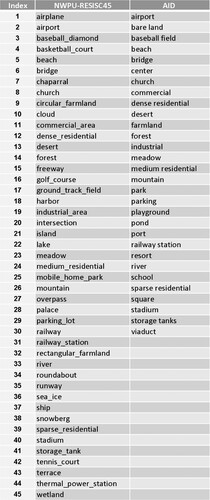
Class indexes given in Figure 1 were used in this research for further analysis. Same index values might be representing different classes due to the differences in the total number of classes. As an example, index number 4 represents basketball court and beach for NWPU-RESISC45 and AID, respectively. Although there are generally common classes in both datasets (e.g. airport, church, stadium, storage tanks, forest, etc.), there are also some differences for the used classes in these datasets (e.g. airplane, tennis court, runway, sea ice is available only in NWPU-RESISC45 whereas pond is available only in AID).

Figure 1. Class index and name of the classes for both data sets.

Table 2 shows the quantitative comparison of experimental results in terms of overall accuracy, overall precision, overall recall, and F1 score for the LCLU classification task on the two above-mentioned datasets. For both data sets, the Baseline method without any ensemble method has lower accuracy values compared to three different DNNE approaches. In particular, the FGE method, despite having a relatively high number of architecture parameters, leads to a relatively low improvement among all DNNEs yet, helps to improve the accuracy of more than two percent compared to the Baseline. SWA, on the other hand, improves the Baseline performance by three percent in both datasets, demonstrates the ability of generalization by performing equally well on images that are acquired from space-borne and air-borne RS platforms. The highest accuracy values were obtained with the SWA ensemble on the AID data set. The number of LCLU classes is 30 in the AID data set, and this is lower than NWPU-RESISC45, which is 45. This emphasizes the impact of the number of classes and their descriptions on classification accuracy.

Table 2. Quantitative comparison of experiments. Bold values indicate the best performance in terms of F1 score.

		Overall accuracy (%)	Precision (%)	Recall (%)	F1 score (%)
NWPU-RESISC45	Baseline	91.36	91.63	91.36	91.49
	SE	94.17	94.20	94.17	94.19
	SWA	94.51	94.51	94.47	94.49
	FGE	93.33	93.41	93.33	93.37
AID	Baseline	94.46	94.51	94.56	94.53
	SE	95.50	95.39	95.24	95.31
	SWA	97.42	97.34	97.28	97.30
	FGE	94.64	94.46	94.40	94.43

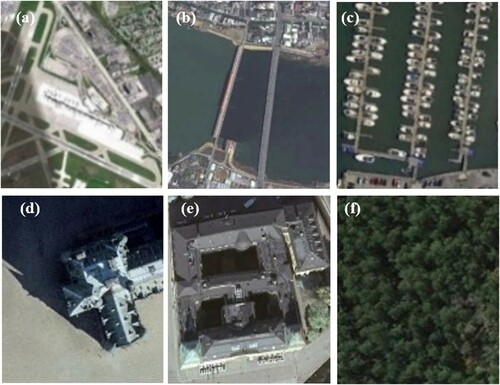
Some of the classification results are presented in Figure 2. Figure 2(a)–(c) are examples of accurate classification results in which the proposed approach performed well for airport, bridge, and harbor instances. On the other hand, Figure 2(d,e) are representing some misclassification examples in which a church was classified as a palace (d), a palace was classified as a church (e), and the forest was classified as wetland (f). Understandably, the classifier struggles to distinguish church and palace classes since both classes look very similar in pattern, structure, and canopy design. Identification of churches and palaces is a challenging task, even in visual interpretation by an expert image analyst. Moreover, for some instances, the classifier fails to capture the characteristic of two land cover classes, forest class and wetland, which can be explained by considering their similarity in texture.

Figure 2. True classifications: (a) Airport, (b) Bridge, and (c) Harbor. Misclassifications: (Ground Truth → Prediction). (d) Church → Palace, (e) Palace → Church, and (f) Forest → Wetland for the NWPU-RESISC45 dataset.

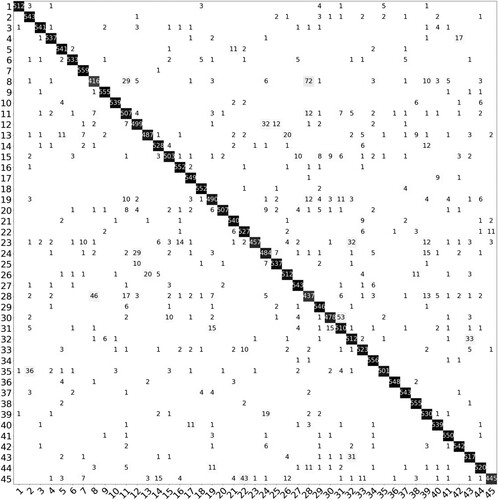
Two confusion matrices were generated to provide a class-wise insight on the performance of the SWA classification approach and are shown in Figures 3 and 4 for AID and NWPU-RESISC45, respectively. For the AID dataset, the challenging classes to classify with the SWA method were: school (25) class which was mainly mixed with commercial (8) class, and resort (23) class which was mainly mixed with park (17) class. The textural, site, and structural characteristics of ‘school and commercial' and ‘resort and park' are very similar, therefore negatively impacting the class identification.

Figure 3. Confusion matrix obtained by using the SWA method for the AID dataset.

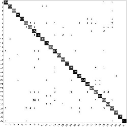
Figure 4. Confusion matrix obtained by using the SWA method for the NWPU-RESISC45 dataset.

The confusion matrix of the AID dataset (Figure 3) shows outstanding results by correctly classifying all of the test images in five classes: storage tanks, mountain, forest, farmland, and beach.

Analysis of the confusion matrix for the NWPU-RESISC45 dataset (Figure 4) illustrated that at most ten test images were misclassified by a model for seven classes: chapparal (559 out of 560 images were correctly classified), circular farmland, golf course, harbor, roundabout, snowberg, storage tank. However, it was challenging to classify some classes such as runway (35), palace (28), and terrace (43) which were confused with bareland (2), church (8), and rectangular farmland (32), respectively.

Zhang, Tang, and Zhao (2019) used AID and NWPU-RESISC45 data sets in their research and compared their proposed VGG-16-CapsNet and Inception-v3-CapsNet approaches with state-of-the-art deep learning classification methods. They achieved 96.32% and 92.6% overall accuracy values with Inception-v3-CapsNet for AID and NWPU-RESISC45, respectively. Our proposed SWA-based ensemble method provides higher overall accuracy values.

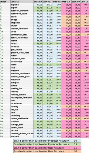
Figure 5 illustrates the UA and PA values for the Baseline and SWA classification of the NWPU-RESISC45 data set. Differences between SWA and Baseline accuracy values are also calculated. Blue colors in Figure 5 represent the class in which SWA results are better than the Baseline approach for PA. For 30 classes, SWA produced better results. For railway, church, beach, wetland, meadow, medium residential, thermal power station, mobile home park, desert, industrial area, terrace, and commercial area classes, the PA value of the proposed SWA method is at least 5% higher than the Baseline approach. For most classes in which the Baseline has higher PA values than the prosed SWA, the increase in accuracy value is very minimal. For the palace class, the PA of the Baseline is 4.35% higher than the SWA; however, this is not the case for UA since the SWA method produced a 16.25% higher accuracy value than the Baseline approach. When all UA values are examined, the SWA method had higher accuracy values for thirty-four different classes. Specifically, for railway station, mountain, rectangular farmland, and palace classes; the increase in UA values are very significant and 9.11%, 12.14%, 13.75%, and 16.25%, respectively. Orange colors in Figure 5 emphasize the classes with higher UA values with the Baseline method; however, the accuracy improvement is very slight being less than 1% for most of them. Finally, there is no class in which the Baseline method simultaneously has higher UA and PA values. On the other hand, for all forty-five classes, the proposed SWA approach exhibited accuracy increase either only for UA or only for PA or for both of them.

Figure 5. User and Producer accuracy values for Baseline and SWA classification.

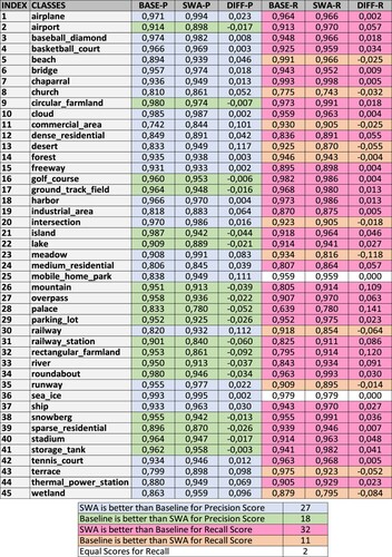
Similarly, by following the same color scheme used in Figure 5, precision (denoted as P in the figure) and recall (denoted as R in the figure) scores of the best-performing ensemble and the baseline approaches were calculated and presented in Figure 6. Our results demonstrate that most of the (32 out of 45) classes are benefited from the SWA approach in terms of recall score. The classes that are most benefitted the most are mountain, rectangular farmland, and palace. As for the precision score, similarly, the SWA approach helped the vast majority (27 out of 45) of the classes to increase their performance.

Figure 6. Precision and recall scores for Baseline and SWA classification.

5. Conclusion

Comparison and inspection of deep ensemble networks have been presented in this research, and utilizing DNNEs was found to be beneficial over individual training schemes for the LCLU classification task. All the methods which use DNNEs perform significantly better performance; information extracted from multiple learners produced improved results compared to the single-training scheme. The experimental results on NWPU-RESISC45 and AID datasets demonstrated that utilizing the aggregated information from SE, SWA and FGE increased the classification performance. Among three different ensemble learners, the SWA method provided the best results in terms of all evaluation metrics. It achieved high performance on two commonly used publicly available RS datasets: NWPU-RESISC45 and AID.

Deployment of DNNE methods in RS image classification has improved the generalizability and robustness of the DNNs and resulted in higher accuracy for a variety of LCLU categories.

Our results demonstrated that the use of DNNE has increased the performance of the LCLU classification task, regardless of the used ensemble method. We accomplished good performance improvement by adopting DNNE techniques, and our results have the potential to assist researchers in achieving better results in RS image classification tasks. Moreover, the benefit of the DNNE provides is data agnostic since both datasets used in this study harnesses from combining multiple learner’s capabilities of classifying LCLU classes to improve the performance. We presented a comparison of DNNE techniques for two public remote sensing datasets, NWPU-RESISC45 and AID to generate benchmark research on the ensemble-based classification that will be a reference for further studies in this task.

Data and codes availability statement

The data that support the findings of this study are openly available in https://figshare.com/s/1e3b4ca24466285e7ac8 at DOI 10.6084/m9.figshare.14703507.

Disclosure statement

No potential conflict of interest was reported by the author(s).

References

- Alganci, Ugur, Gozde Nur Kuru, Irmak Yay Algan, and Elif Sertel. 2019. “Vineyard Site Suitability Analysis by Use of Multicriteria Approach Applied on Geo-Spatial Data.” Geocarto International 34 (12): 1286–1299. doi:https://doi.org/10.1080/10106049.2018.1493156.
- Bishop, Christopher M. 2006. Pattern Recognition and Machine Learning (Information Science and Statistics). Berlin/Heidelberg: Springer-Verlag.
- Cheng, Gong, Xingxing Xie, Junwei Han, Lei Guo, and Gui-Song Xia. 2020. “Remote Sensing Image Scene Classification Meets Deep Learning: Challenges, Methods, Benchmarks, and Opportunities.” IEEE Journal of Selected Topics in Applied Earth Observations and Remote Sensing 13: 3735–3756. doi:https://doi.org/10.1109/JSTARS.2020.3005403.
- Dietterich, Thomas G. 2000. “Ensemble Methods in Machine Learning.” In Multiple Classifier Systems, 1–15. Berlin/Heidelberg: Springer.
- Drucker, Harris, Robert E Schapire, and Patrice Simard. 1993. “Improving Performance in Neural Networks Using a Boosting Algorithm.” Advances in Neural Information Processing Systems 5 (1990): 42–49.
- Garipov, Timur, Pavel Izmailov, Dmitrii Podoprikhin, Dmitry Vetrov, and Andrew Gordon Wilson. 2018. “Loss Surfaces, Mode Connectivity, and Fast Ensembling of DNNs.” ArXiv, no. NeurIPS: 1–10.
- Granitto, P. M., P. F. Verdes, and H. A. Ceccatto. 2005. “Neural Network Ensembles: Evaluation of Aggregation Algorithms.” Artificial Intelligence 163 (2): 139–162. doi:https://doi.org/10.1016/j.artint.2004.09.006.
- He, Kaiming, Xiangyu Zhang, Shaoqing Ren, and Jian Sun. 2016. “Deep Residual Learning for Image Recognition.” Proceedings of the IEEE Computer Society Conference on Computer Vision and Pattern Recognition, 770–778. IEEE. doi:https://doi.org/10.1109/CVPR.2016.90.
- Hinton, G. E., and R. R. Salakhutdinov. 2006. “Reducing the Dimensionality of Data with Neural Networks.” Science 313: 504–507. doi:https://doi.org/10.1126/science.1127647.
- Huang, Gao, Yixuan Li, Geoff Pleiss, Zhuang Liu, John E. Hopcroft, and Kilian Q. Weinberger. 2017. “Snapshot Ensembles: Train 1, Get M for Free.” ArXiv, 1–14.
- Huggins, Jonathan H., Trevor Campbell, and Tamara Broderick. 2016. Advances in Neural Information Processing Systems, 29, 4087–4095. Barcelona.
- Izmailov, Pavel, Dmitrii Podoprikhin, Timur Garipov, Dmitry Vetrov, and Andrew Gordon Wilson. 2018. “Averaging Weights Leads to Wider Optima and Better Generalization.” 34th Conference on Uncertainty in Artificial Intelligence 2018, UAI 2018, 2: 876–885.
- Jia, Deng, Dong Wei, R. Socher, Li-Jia Li, Kai Li, and Li Fei-Fei. 2009. “ImageNet: A Large-Scale Hierarchical Image Database.” IEEE, 248–255. doi:https://doi.org/10.1109/cvprw.2009.5206848.
- Krizhevsky, Alex, Ilya Sutskever, and Geoffrey E Hinton. 2012. “ImageNet Classification with Deep Convolutional Neural Networks.” In Proceedings of the 25th International Conference on Neural Information Processing Systems – Volume 1, NIPS’12, 1097–1105. Red Hook, NY: Curran Associates Inc.
- Lecun, Yann, Yoshua Bengio, and Geoffrey Hinton. 2015. “Deep Learning.” Nature 521 (7553): 436–444. doi:https://doi.org/10.1038/nature14539.
- Lee, Stefan, Senthil Purushwalkam, Michael Cogswell, David Crandall, and Dhruv Batra. 2015. “Why M Heads Are Better than One: Training a Diverse Ensemble of Deep Networks.” http://arxiv.org/abs/1511.06314.
- Liu, Xuning, Yong Zhou, Jiaqi Zhao, Rui Yao, Bing Liu, and Yi Zheng. 2019. “Siamese Convolutional Neural Networks for Remote Sensing Scene Classification.” IEEE Geoscience and Remote Sensing Letters 16 (8): 1200–1204. doi:https://doi.org/10.1109/LGRS.2019.2894399.
- Lowe, David G. 2004. “Distinctive Image Features from Scale-Invariant Keypoints.” International Journal of Computer Vision 60 (2): 91–110. doi:https://doi.org/10.1023/B:VISI.0000029664.99615.94.
- Minetto, Rodrigo, Mauricio Pamplona Segundo, and Sudeep Sarkar. 2019. “Hydra: An Ensemble of Convolutional Neural Networks for Geospatial Land Classification.” IEEE Transactions on Geoscience and Remote Sensing 57 (9): 6530–6541. doi:https://doi.org/10.1109/TGRS.2019.2906883.
- Senthilnath, J., Neelanshi Varia, Akanksha Dokania, Gaotham Anand, and Jón Atli Benediktsson. 2020. “Deep TEC: Deep Transfer Learning with Ensemble Classifier for Road Extraction from UAV Imagery.” Remote Sensing 12 (2): 1–19. doi:https://doi.org/10.3390/rs12020245.
- Sertel, Elif, Raziye Hale Topaloğlu, Betül Şallı, Irmak Yay Algan, and Gül Aslı Aksu. 2018. “Comparison of Landscape Metrics for Three Different Level Land Cover/Land Use Maps.” ISPRS International Journal of Geo-Information 7 (10). doi:https://doi.org/10.3390/ijgi7100408.
- Shakya, Achala, Mantosh Biswas, and Mahesh Pal. 2021. “Parametric Study of Convolutional Neural Network Based Remote Sensing Image Classification.” International Journal of Remote Sensing 42 (7): 2663–2685. doi:https://doi.org/10.1080/01431161.2020.1857877.
- Şimşek, Duygu, and Elif Sertel. 2018. “Spatial Analysis of Two Different Urban Landscapes Using Satellite Images and Landscape Metrics.” Photogrammetric Engineering & Remote Sensing 84 (11): 711–721. doi:https://doi.org/10.14358/PERS.84.11.711.
- Sumbul, Gencer, Marcela Charfuelan, Begum Demir, and Volker Markl. 2019. “Bigearthnet: A Large-Scale Benchmark Archive for Remote Sensing Image Understanding.” 5901–5904. doi:https://doi.org/10.1109/igarss.2019.8900532.
- Szegedy, Christian, Vincent Vanhoucke, Sergey Ioffe, Jon Shlens, and Zbigniew Wojna. 2016. “Rethinking the Inception Architecture for Computer Vision.” In Proceedings of the IEEE Computer Society Conference on Computer Vision and Pattern Recognition 2016-Decem, 2818–2826. IEEE. doi:https://doi.org/10.1109/CVPR.2016.308.
- Torralba, Antonio, and Aude Oliva. 2001. “Modeling the Shape of the Scene: A Holistic Representation of the Spatial Envelope.” International Journal of Computer Vision 42 (3): 145–175.
- Wasay, Abdul, Brian Hentschel, Yuze Liao, Sanyuan Chen, and Stratos Idreos. 2018. “MotherNets: Rapid Deep Ensemble Learning.” http://arxiv.org/abs/1809.04270.
- Xia, Min, Namei Tian, Yonghong Zhang, Yiqing Xu, and Xu Zhang. 2020. “Dilated Multi-Scale Cascade Forest for Satellite Image Classification.” International Journal of Remote Sensing 41 (20): 7779–7800. doi:https://doi.org/10.1080/01431161.2020.1763511.
- Yu, Yunlong, Xianzhi Li, and Fuxian Liu. 2020. “Attention GANs: Unsupervised Deep Feature Learning for Aerial Scene Classification.” IEEE Transactions on Geoscience and Remote Sensing 58 (1): 519–531. doi:https://doi.org/10.1109/TGRS.2019.2937830.
- Yuan, Qiangqiang, Huanfeng Shen, Tongwen Li, Zhiwei Li, Shuwen Li, Yun Jiang, Hongzhang Xu, et al. 2020. “Deep Learning in Environmental Remote Sensing: Achievements and Challenges.” Remote Sensing of Environment 241: 111716. doi:https://doi.org/10.1016/j.rse.2020.111716.
- Zhang, Wei, Ping Tang, and Lijun Zhao. 2019. “Remote Sensing Image Scene Classification Using CNN-CapsNet.” Remote Sensing 11 (5). doi:https://doi.org/10.3390/rs11050494.
- Zhao, Huizhen, Fuxian Liu, Han Zhang, and Zhibing Liang. 2019. “Convolutional Neural Network Based Heterogeneous Transfer Learning for Remote-Sensing Scene Classification.” International Journal of Remote Sensing 40 (22): 8506–8527. doi:https://doi.org/10.1080/01431161.2019.1615652.
- Zhu, Xiao Xiang, Devis Tuia, Lichao Mou, Gui-Song Xia, Liangpei Zhang, Feng Xu, and Friedrich Fraundorfer. 2017. “Deep Learning in Remote Sensing: A Review.” doi:https://doi.org/10.1109/MGRS.2017.2762307.