Historical trends of degradation, loss, and recovery in the tropical forest reserves of Ghana

ABSTRACT

The Upper Guinean Forest region of West Africa, a globally significant biodiversity hotspot, is among the driest and most human-impacted tropical ecosystems. We used Landsat to study forest degradation, loss, and recovery in the forest reserves of Ghana from 2003 to 2019. Annual canopy cover maps were generated using random forests and results were temporally segmented using the LandTrendr algorithm. Canopy cover was predicted with a predicted-observed r² of 0.76, mean absolute error of 12.8%, and mean error of 1.3%. Forest degradation, loss, and recovery were identified as transitions between closed (>60% cover), open (15–60% cover) and low tree cover (< 15% cover) classes. Change was relatively slow from 2003 to 2015, but there was more disturbance than recovery resulting in a gradual decline in closed canopy forests. In 2016, widespread fires associated with El Niño drought caused forest loss and degradation across more than 12% of the moist semi-deciduous and upland evergreen forest types. The workflow was implemented in Google Earth Engine, allowing stakeholders to visualize the results and download summaries. Information about historical disturbances will help to prioritize locations for future studies and target forest protection and restoration activities aimed at increasing resilience.

KEYWORDS:

• Landsat
• random forests
• machine learning
• time series
• LandTrendr
• drought
• wildfire

1. Introduction

Tropical forests provide one of the largest global carbon sinks, with intact forests sequestering 1.02 Pg of carbon per year and forest regrowth taking up an additional 1.72 Pg (Pan et al. 2011). They also furnish habitat for half of the world’s terrestrial plant and animal species and supply vital ecosystem services to much of the world (Malhi et al. 2014). Satellite remote sensing is an essential data source for monitoring tropical forest change. Globally, land conversion to agriculture is a major driver of tropical deforestation (Gibbs et al. 2010), and the capabilities of satellite remote sensing for monitoring land use change and forest loss are well established (Tucker and Townshend 2000). Many of the tropical forests that remain are impacted by anthropogenic and natural disturbances that do not cause complete canopy removal. These disturbances result in degradation, which is broadly defined as change in forest structure and composition that decreases the provision of ecosystem services (Thompson et al. 2013) or reduces ecosystem resilience to future perturbations (Ghazoul et al. 2015). Compared to deforestation, the slower and more subtle effects of degradation are challenging to detect from space using sensors with moderate to high spatial resolution such as MODIS (250–1000 m pixel size) and Landsat (30 m pixel size). Thus, there is a need to improve satellite-based monitoring approaches so that they are sensitive to a broader range of disturbances, including forest degradation. These techniques must also be translated into practical tools that can be used sustainably by stakeholders in tropical regions.

Our overarching goal was to develop a remote sensing application for monitoring long-term forest change in reserved areas located in the tropical forest zone of Ghana. This area is part of the Upper Guinean Forest region, which is a globally significant biodiversity hotspot but is also among the driest (Malhi and Wright 2004) and the most human-impacted (Norris et al. 2010) tropical ecosystems in the world. Almost all of the remaining forest is in reserved areas, which are impacted by legal and illegal timber harvesting, mining, agricultural encroachment, and wildfires (Acheampong et al. 2019; Hawthorne et al. 2012; Dwomoh et al. 2019; Boadi et al. 2016). Because these disturbances often result in the death or removal of individuals or small patches of trees, forest dynamics need to be assessed along a continuum ranging from minor changes in the canopy to complete deforestation. We designed the West Africa Forest Degradation Data (WAForDD) system to meet the needs of the Forestry Commission of Ghana (FCG) for information about historical patterns of deforestation, degradation, and recovery and to provide tools for updating these estimates.

Landsat currently provides the longest historical record of global forest observations, with regular global acquisitions beginning with the Landsat 7 mission in 2000. However, the challenges of working with Landsat data in tropical regions are well known. The visible and infrared spectral range of Landsat can only detect characteristics of the forest overstory and is not sensitive to changes in the midstory and understory canopy layers. Forest degradation affecting individual trees can be challenging to identify because they impact portions of Landsat pixels, and the spectral changes they cause are small relative to other sources of background variation and noise (Negrón-Juárez et al. 2011). Persistent cloud cover also limits the frequency and quality of observation in most tropical forest ecosystems (Potapov et al. 2012; Sannier et al. 2014). Newer satellite missions such as Sentinel-1 and 2 offer advantages such as 10–20 m spatial resolutions (versus 30 m for Landsat), and synthetic aperture radar that can penetrate clouds (Erinjery, Singh, and Kent 2018; Reiche et al. 2018), but lack the long-term record of Landsat. Thus, there is a need for approaches that take advantage of the historical depth of the Landsat archive while minimizing its limitations.

Techniques such as machine learning and time series modelling have emerged as important tools for Landsat data processing and have the potential to improve detection of the subtle signals associated with tropical forest degradation. Machine learning approaches such as random forests, support vector machines, and neural networks are generally more accurate and robust for land cover and land use applications than more traditional classification schemes based on logistic regression, K-means, and maximum likelihood (Yu et al. 2014; Thanh et al. 2020). Time series models are applied at the individual pixel level to smooth noise, interpolate over data gaps caused by clouds and the Landsat 7 scan line corrector failure, and identify disturbances. Some approaches, such as the Breaks for Additive Seasonal and Trend (BFAST) method (Verbesselt et al. 2010) and the Continuous Change Detection and Classification (CCDC) technique (Zhu and Woodcock 2014), model seasonal and interannual trends with regression and detect disturbances based on observed deviations from the model predictions. Other techniques such as the Vegetation Change Tracker (VCT, Huang et al. 2010) and Landsat-based detection of Trends in disturbance and recovery (LandTrendr, Kennedy, Yang, and Cohen 2010) use annual time series of spectral indices to distinguish sudden changes caused by disturbances from periods of relative stability or recovery. Machine learning and time series methods have been combined for terrestrial monitoring applications by first applying time-series methods for processing spectral bands or indices, and then using processed time series as inputs for machine learning algorithms that predict land cover change (Zhu and Woodcock 2014; Cohen et al. 2018; Healey et al. 2018).

A challenge in implementing these methods is the need for computational resources to store and process satellite data. An individual project can require thousands of Landsat images comprising billions of pixels. In many low- and middle-income countries, slow and unstable internet bandwidth can make it impossible to acquire the raw satellite data. The emergence of cloud computing platforms such as Google Earth Engine (GEE) is an important advance that facilitates remote sensing applications (Gorelick et al. 2017). Computationally intensive methods are executed using parallel processing in the Google Cloud, allowing the processing of massive satellite datasets over large areas in settings with limited computational and internet resources. Because of these advantages, GEE has been widely used to develop remote sensing applications in a variety of fields (Tamiminia et al. 2020).

To monitor historical forest degradation, loss, and recovery in Ghana, we developed a novel approach that combined machine-learning predictions with time series modeling. This technique first predicted canopy cover as a continuous land cover variable with random forests and then used LandTrendr for segmented time series regression of predicted canopy cover to identify disturbance and recovery. We developed WAForDD entirely in Google Earth Engine to provide a cloud-based implementation that can be used by the Centre for Remote Sensing and Geographic Information Services (CERSGIS) at the University of Ghana and the FCG. Our objectives were to (1) Assess the potential for using machine learning in combination with Landsat data to predict overstory forest cover in tropical West Africa, (2) Determine whether processing the canopy cover predictions with segmented time series regression improved prediction accuracy, (3) Use the resulting time series of annual canopy cover to identify historical trends and geographic patterns of forest loss, degradation, and recovery, and (4) Develop software to implement the system.

2. Materials and methods

2.1. Study area

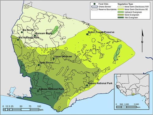
The study area encompassed all designated forest reserves in the moist and wet tropical forest zones of Ghana. These reserved areas covered approximately 1.5 million hectares (Figure 1). There is a strong gradient of decreasing precipitation from southwest to northeast, and the forest types vary along this gradient from wet evergreen to moist evergreen, moist semi deciduous, and dry semi-deciduous. With the exception of several national parks and wildlife reserves, most forest reserves are actively managed for timber production. Harvesting is mainly single-tree and small-group selection on a 40-year cutting cycle (Hawthorne et al. 2012). Illegal logging is widespread and has been estimated to remove as much timber as legal logging (Hansen and Treue 2008). There is also agricultural encroachment in many reserves, including legally admitted farms and agroforestry systems (taungya) as well as illegal land clearing and farming (Acheampong et al. 2019). Fire is used for agricultural land clearing throughout the forest zone, but generally does not spread into the closed canopy forests (Dwomoh and Wimberly 2017b). However, forests are more susceptible to fire during droughts (Hawthorne 1994; Dwomoh et al. 2019). Forest canopy loss makes forests more vulnerable to fire and can initiate a positive feedback loop of fire encroachment that causes more forest degradation, ultimately resulting in conversion from forest to shrub and grass cover (Dwomoh and Wimberly 2017a).

Figure 1. Map of the study area with vegetation types and forest reserve boundaries. Reserves mentioned in the text and summarized in Figures 4 and 5 are labelled for reference. The study area encompasses the moist and wet closed-canopy forest vegetation types as defined in Hall and Swaine (1976).

2.2. Landsat data

We used all available Landsat 7 (ETM+) and Landsat 8 (OLI) data from 2001 to 2020 for the study area, which included 2,713 individual Landsat images (Table S1). To maximize spatial and temporal consistency, we used surface reflectance level-2 science products from Landsat Collection 2. Surface reflectance was generated using the Landsat Ecosystem Disturbance Adaptive Processing System (LEDAPS) for Landsat 7 and the Landsat Surface Reflectance Code (LaSRC) for Landsat 8. All data processing was carried out using Google Earth Engine (Gorelick et al. 2017), with the exception of endmember selection for spectral mixture analysis, which was done using ENVI.

All visible, near infrared, and shortwave-infrared bands were utilized along with the pixel quality assessment band (pixel_qa). We used the method of Roy et al. (2016) to cross-calibrate Landsat 8 reflectance with Landsat 7 reflectance to correct for sensor differences and generate a harmonized dataset. This correction used linear calibration functions to make relatively small adjustments to reflectance to account for changes in the frequency ranges of the spectral bands and the dynamic range of the sensor. Pixels identified as cloud, cloud shadow, or water were masked out using the pixel_qa layer. These cloud screening flags were generated using the FMASK algorithm (Zhu, Wang, and Woodcock 2015). However, an initial assessment found that the pixel_qa band often missed areas with clouds and haze. As additional screens, we masked out all pixels with a reflectance value greater than 0.09 in the blue band, and we applied another cloud mask derived from spectral mixture analysis using the cloud endmember from Souza et al. (2013).

2.3. Spectral index calculation and image compositing

We used linear spectral mixture analysis (SMA) to partition the spectral signature of each pixel into four fractions: green vegetation (GV), non-photosynthesizing vegetation (NPV), soil (SO), and shade (SH). Endmembers for GV, NPV, and SO were selected by first identifying endmember candidates from a clear sky Landsat image using SMACC Endmember Selection in ENVI 5.1. Then, final endmembers (Table S2) were determined based upon the spectral shape, image context and root mean squared errors (RMSEs) of the resulting fraction images following Numata et al. (2007) and Souza et al. (2013). The RMSE quantifies the differences between observed reflectance and predicted reflectance as a linear function of the spectral endmembers. These endmembers were then used to calculate GV, NPV, and SO fractions for each pixel using the image.unmix() function in Google Earth Engine (GEE), and the SH fraction was calculated by subtracting the sum of these three fractions from 100%.

The normalized difference fraction index (NDFI) was used as an indicator of forest canopy structure (Table 1). This index has previously been applied to monitor forest loss and degradation in the Amazon (Souza, Roberts, and Cochrane 2005; Souza et al. 2013; Bullock, Woodcock, and Olofsson 2020). The NDFI value is highest in pixels with large values of GV and SH and small values of NPV and SO. This index normalizes GV for the effects of SH, and is typically high in mature, intact forests where a continuous canopy with large tree crowns creates a mixture of green vegetation and shadow. In contrast, the NDFI is lower in situations where tree loss decreases the amount of GV and increases the exposure of NPV and SO (Souza, Roberts, and Cochrane 2005).

Table 1. Spectral indices used in random forests modeling of canopy cover in forests reserves in Ghana.

Abbreviation	Spectral Index	Description	Reference
B1-5, B7	Surface reflectance	Surface reflectance from Landsat specified using ETM+ band numbers^a	(United States Geological Survey 2020)
GV	Green vegetation fraction	Derived from spectral mixture analysis using all visible and infrared spectral bands	(Souza, Roberts, and Cochrane 2005)
NPV	Non-photosynthesizing vegetation fraction	Derived from spectral mixture analysis using all visible and infrared spectral bands	(Souza, Roberts, and Cochrane 2005)
SO	Soil fraction	Derived from spectral mixture analysis using all visible and infrared spectral bands	(Souza, Roberts, and Cochrane 2005)
SH	Shade fraction	Derived from spectral mixture analysis using all visible and infrared spectral bands	(Souza, Roberts, and Cochrane 2005)
NDFI	Normalized difference fraction index	$\mathrm{N}\mathrm{D}\mathrm{F}\mathrm{I}={\displaystyle \frac{\mathrm{G}{\mathrm{V}}_{\mathrm{S}\mathrm{H}}-\left(\mathrm{N}\mathrm{P}\mathrm{V}+\mathrm{S}\mathrm{O}\right)}{\mathrm{G}{\mathrm{V}}_{\mathrm{S}\mathrm{H}}+\mathrm{N}\mathrm{P}\mathrm{V}+\mathrm{S}\mathrm{O}}}$, where $\mathrm{G}{\mathrm{V}}_{\mathrm{S}\mathrm{H}}={\displaystyle \frac{\mathrm{G}\mathrm{V}}{100\text{-}\mathrm{S}\mathrm{H}}}$	(Souza, Roberts, and Cochrane 2005)
NDFI2	Normalized difference fraction index (version 2)	$\mathrm{N}\mathrm{D}\mathrm{F}\mathrm{I}2={\displaystyle \frac{\mathrm{S}\mathrm{H}-\left(\mathrm{N}\mathrm{P}\mathrm{V}+\mathrm{S}\mathrm{O}\right)}{\mathrm{S}\mathrm{H}+\mathrm{N}\mathrm{P}\mathrm{V}+\mathrm{S}\mathrm{O}}}$	Developed for this study
NDVI	Normalized difference vegetation index	$\mathrm{N}\mathrm{D}\mathrm{V}\mathrm{I}={\displaystyle \frac{\mathrm{B}4-\mathrm{B}3}{\mathrm{B}4+\mathrm{B}3}}$	(Tucker 1979)
EVI2	Two-band enhanced vegetation index	$\mathrm{E}\mathrm{V}\mathrm{I}2=2.4{\displaystyle \frac{\mathrm{B}4-\mathrm{B}3}{\mathrm{B}4+\mathrm{B}3+1}}$	(Jiang et al. 2008)
NBR	Normalized burn ratio	$\mathrm{N}\mathrm{B}\mathrm{R}={\displaystyle \frac{\mathrm{B}4-\mathrm{B}7}{\mathrm{B}4+\mathrm{B}7}}$	(López García and Caselles 1991)
NDWI	Normalized difference water index	$\mathrm{N}\mathrm{D}\mathrm{W}\mathrm{I}={\displaystyle \frac{\mathrm{B}2-\mathrm{B}4}{\mathrm{B}2+\mathrm{B}4}}$	(McFeeters 1996)
NDMI	Normalized difference moisture index	$\mathrm{N}\mathrm{D}\mathrm{M}\mathrm{I}={\displaystyle \frac{\mathrm{B}4-\mathrm{B}5}{\mathrm{B}4+\mathrm{B}5}}$	(Gao 1996)
TCB	Tasseled cap brightness	Linear combination of all visible and infrared spectral bands	(Huang et al. 2002)
TCG	Tasseled cap greenness	Linear combination of all visible and infrared spectral bands	(Huang et al. 2002)
TCW	Tasseled cap wetness	Linear combination of all visible and infrared spectral bands	(Huang et al. 2002)

^a Harmonized Landsat 7 (ETM+) and Landsat 8 (OLI) data were used to compute all indices, and the OLI data were converted to the ETM+ band numbering scheme.

We also calculated NDFI2, a modified version of NDFI that we developed for this study. NDFI2 is similar to NDFI but replaces the GV_sh fraction with the SH fraction (Table 1) and is thus primarily sensitive to the contrast between dark shadows created by the irregular forest canopy and relatively bright material such as SO and NPV. These six spectral indices (GV, NPV, SO, SH, NDFI and NDFI2) were used as predictor variables for canopy cover modeling using random forests. In addition, we used the raw spectral bands and calculated a variety of other spectral indices commonly used for forest mapping (Table 1). These included the normalized difference vegetation index (NDVI, Tucker 1979), two-band enhanced vegetation index (EVI2; Jiang et al. 2008), normalized burn ratio (NBR, López García and Caselles 1991), two variants of the normalized difference water index (NDWI) designed to detect open water bodies (McFeeters 1996) and the water content of vegetation (Gao 1996), and the brightness (TCB), greenness (TCG), and wetness (TCW) indices derived from the tasselled cap transformation (Huang et al. 2002). The spectral indices were composited annually for all years from 2001 to 2020 using an annual median filter. A 3 × 3 pixel (0.81 ha) mean spatial filter was applied to the annual composites to rescale the spectral data to approximate the 1 ha minimum mapping unit used by the FCG to classify forests based on canopy cover.

2.4. Training and validation data

We created a spatial database of percent canopy cover from very-high resolution (VHR) imagery obtained through Google Earth and from the NASA high-resolution data archive, primarily WorldView and other data sources with a spatial resolution finer than 2 m. Sample points were constrained to the areas of forest and game reserves within the study area. Within these areas, we generated a simple random sample of Landsat pixels to represent the centers of the sample plots. Around these pixels, we created sample plot polygons the size of 3 × 3 Landsat pixels (0.81 ha).

The availability of historical VHR satellite data varied over space and time because most commercial satellites do not acquire regular imagery from rural tropical locations. At each random location, we took canopy cover measurements for all years in which VHR imagery were available. If there were no VHR images for a given location, we skipped it and moved to the next random location. We used the VHR imagery to estimate percent forest canopy cover as the area of the sample plot covered by the overstory tree canopy (Figure S1). Estimates ranged from 0% to 100%, in 5% increments. Two interpreters were trained by individuals with field experience in Ghanaian forests, and an extensive library of georeferenced field photographs was available to support the interpretation. In total, 5,543 sample units were randomly collected from the study region with dates between 2010 and 2017. There were 170 points in 2010, 223 points in 2011, 497 points in 2012, 900 points in 2013, 313 points in 2014, 2040 points in 2015, 741 points in 2016, and 659 points in 2017. These data were randomly split into a training dataset with 2771 points that was used for model fitting, and a separate validation dataset with 2772 points that was used for accuracy assessment.

2.5. Canopy cover prediction with random forests

We mapped canopy cover classes by modeling relationships between Landsat-derived spectral indices and canopy cover measurements from the VHR imagery. We used the random forests regression algorithm (Breiman 2001), a tree-based ensemble machine learning algorithm, to predict canopy cover. Random forests generate predictions by creating a set of regression trees and aggregating their results to improve prediction accuracy. The regression trees use recursive partitioning to split the data into branches based on the predictor variables, and the resulting set of decision rules is used to determine the response for a given set of predictors. Each tree is based on a random sample with replacement taken from the original dataset and uses a random subset of the explanatory variables to develop the trees. These procedures decrease the correlations among trees in the ensemble and increase the accuracy of the ensemble prediction that is generated by averaging across the trees.

To train the random forests model, we extracted the Landsat spectral indices corresponding to sample plots from the corresponding location and year in the training dataset. We ran the random forests regression model using the smileRandomForest() function in GEE with an ensemble size of 1000 trees, a bag fraction of 0.67, variables per split equal to the number of predictor variables divided by three, and a minimum node size of five. We then applied this model to predict percent canopy cover across the entire study area for all years from 2001 to 2020. We estimated the relative importance of each predictor variable based on the increase in residual sum of squares when each variable was excluded from the model.

2.6. Temporal segmentation with LandTrendr

After creating the annual canopy cover datasets, we applied the LandTrendr temporal segmentation algorithm (Kennedy, Yang, and Cohen 2010) in GEE to process the resulting time series on an individual pixel basis. LandTrendr employs statistical fitting algorithms to concisely describe a noisy time series using segmented linear regression and point-to-point interpolation, thereby capturing the major patterns of change in the time series while smoothing undesired random noise caused by normal phenological variation, year-to-year climate fluctuations, atmospheric effects, and sun angle (Kennedy, Yang, and Cohen 2010; Kennedy et al. 2012). When applied to a time-series stack, LandTrendr identifies break points in the temporal trajectory that distinguish periods of relatively consistent change trajectories. To select parameters for the LandTrendr algorithm (Table S3) we first ran the algorithm with the default values and then conducted a sensitivity analysis in which we systematically adjusted the parameters and visually examined time series patterns in locations with known disturbance histories. The source values of observations fitted to segment lines between vertices (FTV) complete annual time series from the LandTrendr algorithm were then used as the final estimates of canopy cover for each pixel-year combination.

2.7. Model evaluation

We used the validation dataset to carry out a multi-year evaluation of the canopy cover predictions. We evaluated the predictions generated by the random forests model, and the predictions after segmented regression with LandTrendr. Accuracy statistics included mean error (ME), mean absolute error (MAE), root mean squared error (RMSE), and the r² of the predicted-observed regression (Bennett et al. 2013). ME indicates whether predictions are systematically higher or lower than observations. MAE and RMSE both measure how close predictions are to observations with lower values indicating higher accuracy, but RMSE is more sensitive to large deviations. The predicted-observed r² measures the degree to which the observations can be modeled as a linear function of the predictions. We used a bootstrap approach with 10,000 samples to estimate the 95% confidence interval of all these accuracy statistics.

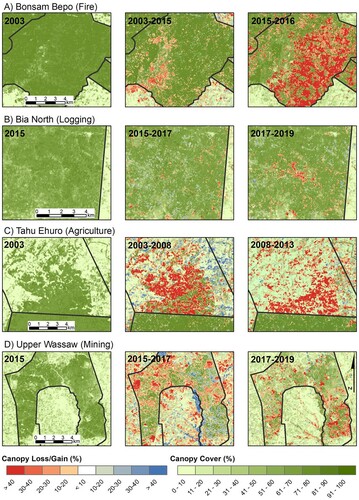
We also evaluated change in several locations with known disturbance histories (Figure 1). We selected three national parks (Ankasa, Bia, and Kakum) and parts of one forest reserve (Bobiri) designated for conservation and research. In these locations, logging is expected to be minimal and no known fires have occurred throughout the study period. In Bia North, we identified a portion of the reserve where widespread logging beginning in 2017 was clearly visible in the available VHR imagery. In the southern portion of the Tano Ehuro reserve, we identified an area where agricultural encroachment occurred in the late 2000s and early 2010s (Owubah, Donkor, and Nsenkyire 2000). In Bonsam Bepo, there was widespread fire in 2016 associated with the 2015–2016 El Niño-Southern Oscillation (ENSO) drought, as documented by burn scars in Landsat imagery as well as active fire detections from MODIS and VIIRS (Dwomoh et al. 2019). In the eastern portion of Upper Wassaw, we identified an area where there was known to be widespread forest degradation and loss from illegal mining operations in 2019. We mapped the changes in canopy cover in these areas and graphed change events over time using the methods described in the next section.

2.8. Change detection

The continuous canopy cover data from the LandTrendr FTV complete annual time series were used to classify forests into three classes: low tree cover (0–15%) open forest (15–60%) and closed forest (> 60%), and changes were based on transitions among these classes. This approach is different from the more common application of LandTrendr for disturbance detection, in which breakpoints identified by the segmented regression analysis are used to identify the timing of disturbances. This modification was necessary to meet the requirements of the FCG, which defines change types based on specific canopy cover thresholds. The rationale behind using the predicted canopy cover values from the LandTrendr algorithm was to reduce noise in the canopy cover time series and better distinguish periods of relative stability from more rapid changes resulting from disturbance and recovery.

The canopy cover classes were used to define five change types. Change from closed to open forest was characterized as forest degradation. Change from either closed or open forest to low tree cover was characterized as closed forest loss or open forest loss, respectively. Change from low tree cover to open forest was characterized as open forest recovery and change from open to closed forest was characterized as closed forest recovery. An additional rule was applied in which these changes were only considered valid if a pixel remained in the new state for two or more years. For example, if a pixel was degraded, but then immediately recovered to a closed forest state the next year, this change was not considered biologically realistic and the forest was assumed to have remained in a closed forest state. Applying these rules to annual canopy cover data from 2001 to 2020, we generated change events for 2003–2019. We summarized the areas affected by these changes by year and ecoregion to assess trends in disturbance and recovery over time. We also summarized the total area affected by these change types for each forest reserve to assess geographic patterns in change trajectories throughout the forest zone of Ghana.

2.9. Implementation

The WAForDD system was implemented entirely using Google Earth Engine (GEE), a cloud-based system for satellite image processing that is accessible through a web browser interface (Gorelick et al. 2017; Kennedy et al. 2018). The motivation behind this implementation was the need for a system that could be transferred to geospatial scientists and forest managers in Ghana for sustainable use. GEE was particularly suitable because the browser-based JavaScript API provides access to all the necessary algorithms for data retrieval, canopy cover estimates, and time series modeling with LandTrendr, while the cloud-based processing environment provides sufficient computational resources and does not require downloading of large volumes of data to local systems. The WAForDD application was implemented using four GEE scripts for: (1) Generating annual composites of Landsat 7 and 8 data, (2) Predicting annual canopy cover with random forests, (3) Running LandTrendr on the annual canopy cover estimates, and (4) Generating annual estimates of forest degradation, loss, and recovery. The output from each of these scripts was stored in the cloud as a GEE asset. The first three scripts were designed to be run in the GEE code editor, while the fourth script was implemented as an Earth Engine App (https://mcwimberly.users.earthengine.app/view/wafordd22), which provides a user-friendly interface for visualizing the results through maps and time series charts.

3. Results

3.1. Canopy cover predictions

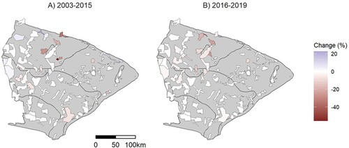
We compared random forests model including all possible spectral variables with alternative models based on subsets of these variables, including the SMA variables, the tasseled cap variables, and the normalized difference indices. In all cases, the model including all spectral variables had higher accuracy than models based on subsets, and we used this model to generate canopy cover predictions and evaluate their accuracy. After processing the canopy cover estimates from the random forests model with LandTrendr, prediction errors measured by MAE and RMSE decreased slightly (Table 2). The strength of association between predicted and observed variables measured by the r² also increased, and the bias of the canopy cover predictions measured by ME increased slightly. Plots showing the relationships between observed and predicted values are provided in Figure S2. The LandTrendr processed canopy cover estimates were used to generate annual maps of canopy cover. To illustrate the outputs, Figure 2 shows the map of canopy cover in 2003 with change in canopy cover from 2003 to 2015, and Figure 3 shows the map of canopy cover in 2015 with change in canopy cover from 2015 to 2019.

Figure 2. Change in canopy cover from 2003 to 2015. Black lines are the boundaries of vegetation types from Figure 1. Percent loss or gain values greater than 10% are overlaid on a map of 2003 canopy cover.

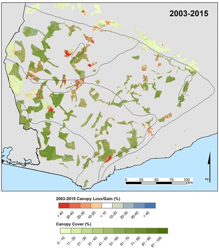
Figure 3. Change in canopy cover from 2015 to 2019. Black lines are the boundaries of vegetation types from Figure 1. Percent loss or gain values greater than 10% are overlaid on a map of 2015 canopy cover.

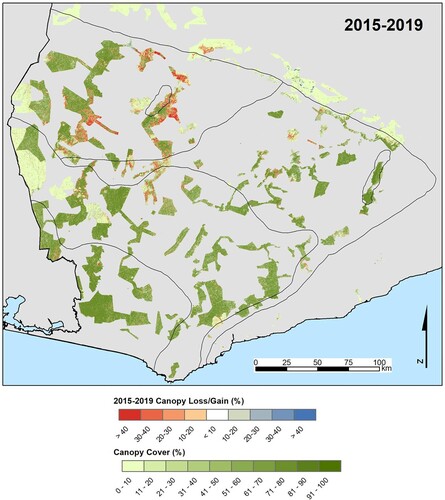
Table 2. Accuracy statistics for percent canopy cover predictions using two methods.^a

Accuracy Statistic	Random Forests^a	Random Forests + LandTrendr
Mean Error (%)	0.85 (0.17-1.52)	1.3 (0.71-1.99)
Mean Absolute Error (%)	13.0 (12.6-13.5)	12.8 (12.4-13.2)
Root Mean Squared Error (%)	17.9 (17.2, 18.5)	17.0 (16.5-17.5)
Predicted-Observed r^2	0.73 (0.71-0.75)	0.76 (0.74-0.78)

^a Numbers in parentheses are 95% confidence intervals.

Surface reflectance from one of the shortwave infrared bands (B5) was the most important predictor of canopy cover followed by TCW, which is sensitive to the contrast between the near infrared and shortwave infrared bands (Table 3). The new NDFI2 index developed for this study had the third highest importance followed by another shortwave infrared band (B7) and the TCB, NDFI, and NPV indices. All other variables had relatively low importance, and the three indices measuring vegetation greenness: (TCG, NDVI, and GV) had the lowest importance out of all variables.

Table 3. Relative importance of spectral variables in the random forests model of canopy cover.

Predictor Variable^a	Importance^b
B5	1.000
TCW	0.638
NDFI2	0.427
B7	0.393
TCB	0.216
NDFI	0.213
NPV	0.165
B2	0.091
NDMI	0.081
B1	0.066
EVI2	0.066
SOIL	0.059
B3	0.056
SHADE	0.055
NBR	0.053
NDWI	0.052
NIR	0.050
NDVI	0.049
GV	0.049
TCG	0.046

^a Variable codes are defined in Table 1.

^b Calculated as the increase in sum of squared errors (SSE) when each variable was excluded from the model and expressed as a proportion of the increased SEE of the most important variable.

3.2. Change trajectories

In areas that were protected from disturbance, forests were primarily closed canopy and remained relatively stable throughout the study period (Figure 4(a–d)). Small amounts of degradation and recovery observed in the protected areas were likely the result of natural gap disturbance processes. In disturbed areas, the timing of observed changes in canopy cover corresponded with dates of known disturbance events (Figure 4(e–h), Figure 5). Fire was widespread across Bonsam Bepo in 2016 (Figure 4(e), Figure 5(a)), there was a sharp increase in degradation in 2016 followed by lower levels of disturbance and recovery in subsequent years. In Bia North (Figure 4(f), Figure 5(b)), logging activity beginning in 2017 resulted in increased forest degradation. In Tano Ehuro (Figure 4(e) and Figure 5(c)) agricultural encroachment led to the widespread loss of forest cover (Owubah, Donkor, and Nsenkyire 2000). Substantial blocks of closed-canopy forest remained in the southern portion of Tano Ehuro in 2003, but were rapidly lost over the next decade. Most change events from 2005 to 2008 were forest degradation, followed by higher levels of forest loss from 2009 to 2013. In the eastern portion of Upper Wassaw (Figure 4(h) and Figure 5(d)), there was some disturbance and recovery prior to 2017. However, degradation and forest loss increased considerably in 2019 because of illegal mining activities in the reserve.

Figure 4. Time series of canopy cover from eight locations with known disturbance histories. (a–d) are national parks and preserves where change is expected to be minimal. E-H are forest reserves where different types of disturbances have occurred. Locations are shown in Figure 1.

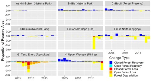
Figure 5. Changes in canopy cover in four reserves with known disturbance histories. Different dates were selected for each reserve to highlight conditions before and after disturbances. (a) Wildfire in Bonsam Bepo, (b) Logging in Bia North, (c) Agricultural encroachment in Tano Ehuro, (d) Artisanal mining in Upper Wassaw. Locations are shown in Figure 1. Percent loss or gain values greater than 10% are overlaid on maps of canopy cover at the beginning of each period.

3.3. Trends of disturbance and recovery

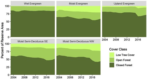
Reserved areas in all vegetation types were dominated by closed forest in 2003, with the highest abundances of closed forest (> 75%) in the wet evergreen and upland evergreen types and lower abundances (between 60 and 70%) in the moist evergreen and moist semi-deciduous types (Figure 6). The highest abundances of the low tree cover class were also found in the moist evergreen and moist semi-deciduous types. Closed forest cover was relatively stable over time in the wet evergreen type but decreased in the other vegetation types. The decreases were gradual through 2015, followed by sharper declines beginning in 2016, particularly in the upland evergreen and moist semi-deciduous NW types. There was also some recovery of closed canopy forests after 2016.

Figure 6. Time series of the relative amounts of Low Tree Cover, Open Forest, and Closed Forest summarized by vegetation type.

From 2003 to 2019, we estimated 5493 km² of closed forest degradation along with 2276 km² of total forest loss, including 287 km² of closed forest loss plus 1989 km² of open forest loss (Table 4). Also during this period, there was an estimated 4938 km² of closed forest recovery and 1595 km² of open forest recovery, resulting in a net decline of 842 km² of closed forest and 394 km² of open forest.

Table 4. Estimated areas (in km²) of forest reserves in Ghana affected by disturbance and recovery, summarized for two periods by vegetation type.

Time Period	Type^a	Closed Forest				Open Forest
		Degradation	Loss	Recovery	Net	Loss	Recovery	Net
2003–2015	ME	1721	87	1648	−159	720	680	−40
	MSNW	957	45	898	−105	488	400	−87
	MSSE	794	38	646	−186	223	222	−2
	UE	56	1	53	−3	6	10	3
	WE	512	8	617	97	29	21	−8
	Total	4039	180	3863	−356	1467	1333	−134
2016–2019	ME	470	11	489	8	128	70	−58
	MSNW	643	69	265	−447	266	112	−154
	MSSE	181	18	190	−9	109	70	−39
	UE	26	7	16	−17	10	5	−5
	WE	134	2	115	−21	9	6	−4
	Total	1454	107	1075	−486	522	262	−260
Grand Total		5493	287	4938	−842	1989	1595	−394

^a ME, moist evergreen; MSNW, moist semi-deciduous northwest; MSSE, moist semi-deciduous southeast; UE, upland evergreen; WE, wet evergreen.

From 2003 to 2015, there were relatively small amounts (< 5% of the total area) of annual forest degradation, loss, and recovery observed in the forest reserves each year (Figure 7). However, over this period, the combined area of forest degradation and closed forest loss exceeded closed forest recovery in the moist evergreen, moist semi-deciduous and upland evergreen types, resulting in an overall reduction of closed forest in these vegetation types (Table 4). Similarly, the area of open forest loss exceeded the area of open forest recovery in the moist evergreen, moist semi-deciduous and wet evergreen vegetation types, with the most net open forest loss occurring in the moist semi-deciduous NW types.

Figure 7. Time series of the annual areas of disturbance and recovery events summarized by vegetation type.

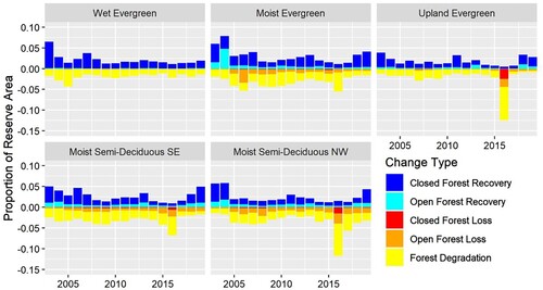
The 2016 El-Nino drought and the associated fires affected the highest percentages of reserve areas in the moist semi-deciduous NW and upland evergreen types (Figure 7). However, because of the small extent of the upland evergreen type, it accounted for a relatively small area of forest degradation and loss from 2016 to 2019 (Table 4). Most of the forest loss and degradation during this time occurred in the moist evergreen, moist semi-deciduous NW, and moist semi-deciduous SE types. In particular, most of the closed forest loss and open forest loss was concentrated in the moist semi-deciduous NW vegetation type.

3.4. Geographic patterns of disturbance and recovery

Summary maps of closed forest change (Figure 8) and open forest change (Figure 9) showed that net change was close to zero in most reserves, with decreases in closed and open forest concentrated in the moist semi-deciduous NW type and the western portion of the moist evergreen type. There were also a number of reserves in the moist semi-deciduous SE type that showed net declines in closed canopy forest in 2003–2015 (Figure 8(a)). Many of the reserves that exhibited net declines in open and closed canopy forest in 2003–2015 (Figure 8(a) and Figure 9(a)) were the same reserves that had net declines in 2016–2019 following the regional drought and fire event (Figure 8(b) and Figure 9(b)). In contrast other reserves such as Tano Ehuro experienced declines before 2016 but were relatively stable from 2016 to 2019 because there was no forest cover remaining.

Figure 8. Maps of net closed forest change summarized by forest reserve for two periods. Change is the area of closed forest recovery minus the total area of closed forest degradation and loss, normalized as a percent of reserve area. Black lines are the boundaries of vegetation types from Figure 1.

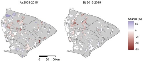
Figure 9. Maps of net open forest change summarized by forest reserve for two periods. Change is the area of open forest recovery minus the area of open forest loss, normalized as a percent of reserve area. Black lines are the boundaries of vegetation types from Figure 1.

4. Discussion

4.1. Disturbance history and forest dynamics in Ghana

This record of change in the forest reserves of Ghana highlights the dynamic nature of these landscapes. From 2003 to 2015, a relatively small portion of the reserves (< 5%) was disturbed each year, with disturbance rates typically higher in the moist semi-deciduous and moist evergreen forest types than in the wet evergreen and upland evergreen types. Open and closed forest recovery also occurred every year, but the cumulative amount of recovery was less than that of degradation and forest loss, resulting in a decline of closed forests and increases in low tree cover and open forests. Many forest reserves, particularly those located in the moist semi-deciduous vegetation types, were already heavily degraded by logging, fire, and agricultural encroachment in the 1980s (Hawthorne and Abu-Juam 1995; Janssen et al. 2018). Our analysis found that most of these reserves maintained closed canopies from 2003 to 2015, emphasizing their resilience to past disturbance. However, even during this period of relative stability, the overall dynamic was a gradual trend of decreasing closed forest. This finding is consistent with other studies that have reported decreasing forest cover in a smaller subregion of Ghana between 2003 and 2018 (Coulter et al. 2016; Tsai et al. 2019) and a broader trend of decreasing forest cover across the entire Upper Guinean Forest Region from 2001 to 2015 (Liu, Wimberly, and Dwomoh 2017).

The 2015–2016 ENSO event and the associated West African drought and wildfires were seminal events within the period of our study, and the net areas of open and closed forest loss and degradation from 2016 to 2019 were greater than the changes that occurred over the preceding 13 years. In 2016, MODIS active fire detections inside forest reserves were much higher than in any previous year since 2003, and were particularly high in the moist semi-deciduous forest types (Dwomoh et al. 2019). The exceptionally strong 1982–1983 ENSO was similarly associated with extensive fire encroachment into forest reserves (Hawthorne 1994). Although sufficient data are not available to compare these two fire events, the historical record does emphasize the importance of infrequent drought years with high fire activity. Thus, there is a need for long-term historical assessments that capture climate anomalies and their impacts, as well as annual monitoring to track where new disturbances are occurring. Specifically, there is concern that disturbances can trigger positive feedback loops of fire and degradation that gradually lead to complete forest loss, which occurred in some reserves in the 1980s (Dwomoh and Wimberly 2017a; Janssen et al. 2018; Brando et al. 2014). Early detection of these trends with satellite remote sensing can be used to target management activities aimed at breaking the cycle of fire and degradation.

We documented considerable recovery of closed-canopy forests in the three years after 2016. This finding supports the conclusions of Bennett et al. (2021) that African tropical forests may have greater resilience to drought than tropical forests in other parts of the world. Rapid recovery of the forest canopy is expected given the potential for rapid growth and crown expansion of tropical trees following disturbance. Some of this recovery may also reflect the direct effects of drought. Many tropical trees can shed leaves to prevent excessive moisture loss when water potential decreases, and flushing of new leaves after the end of the drought would rapidly increase canopy cover (Wolfe, Sperry, and Kursar 2016).

Our change detection was based solely on overstory canopy characteristics that can be observed with optical-infrared sensors. Disturbances, including fire as well as logging and agricultural encroachment, can have a myriad of other impacts that include shifts in species composition, changes in forest structure, declines in productivity and carbon storage, and increasing susceptibility to future disturbances (Ghazoul et al. 2015; Laurin, Hawthorne, et al. 2016). Therefore, rapid recovery of the overstory canopy following the 2016 drought and fires should not be interpreted as return to the pre-fire forest condition. Despite this limitation, Landsat-derived estimates of historical disturbance and recovery are still a valuable source of information. Areas that have been recently or repeatedly disturbed can be targeted for field assessments or in-depth analysis using additional types of remote sensing data such as Lidar (Laurin, Puletti, Chen, et al. 2016), very-high resolution imagery (Wagner et al. 2018; Ferreira et al. 2019), or hyperspectral imagery (Laurin, Puletti, Hawthorne, et al. 2016).

4.2. Methods for estimating forest cover change

The most important spectral variables for predicting canopy cover included reflectance in the shortwave infrared bands as well as TCW, which is sensitive to shortwave infrared reflectance. In contrast, greenness indices such as NDVI, GV, and TCG had the lowest importance values. These results are in line with previous research, which found that TCW and other SWIR-based indices are better predictors of canopy cover and other forest structural attributes than NDVI and similar greenness indices (Czerwinski, King, and Mitchell 2014; Liu, Wimberly, and Dwomoh 2017; Cohen and Spies 1992; Dymond, Mladenoff, and Radeloff 2002). Although NDVI is a strong indicator of woody plant cover across much of central and southern Africa, this relationship is weaker in West Africa where herbaceous plants account for a larger proportion of green vegetation (Mitchard and Flintrop 2013). In Ghana, we observed that croplands and grasslands often had higher NDVI values than forests, where much of the greenness signal was attenuated by the shading effects of multilayered forest canopies. Thus, we found that the NDFI2 index, a modified version of NDFI that excluded the greenness component and was sensitive to the ratio of shade to bright non-photosynthesizing vegetation and soils, was one of the most importance predictors of canopy cover and was a better predictor than the original NDFI index. Based on these results, we recommend that remote sensing research on the dynamics of West African forests should focus on indices that are sensitive to forest canopy moisture and shading rather than green vegetation.

We found that post-hoc processing of annual canopy cover predictions from random forests using segmented regression with the LandTrendr algorithm increased the accuracy of the predictions. From visual examination of the predicted times series from LandTrendr, it was evident that this improvement occurred because anomalously high or low canopy cover predictions that occurred during periods of relative stability were smoothed, whereas the longer-term effects of disturbance on canopy cover were captured by the segmented regression. Most previous studies that combined time series modeling with machine learning for land cover classification (Zhu and Woodcock 2014; Cohen et al. 2018; Healey et al. 2018) have first applied time series methods to one or more spectral variables and then used the outputs as predictor variables in machine learning algorithms for classifying land cover change. In contrast, we first applied the random forests regression model to generate predictions of canopy cover and then used LandTrendr for temporal segmentation as the second step. This approach is similar to the methods used by Main-Knorn et al. (2013) to model coniferous forest biomass change in eastern Europe and by Hu and Hu (2020) to model classification probabilities for land cover classes in Russia. It was straightforward to implement as a series of modular scripts in GEE and efficient enough for annual updates to be made with only a few hours of computation time. To our knowledge, this is the first application of this approach for tracking forest degradation in tropical regions.

The LandTrendr algorithm was originally developed and applied in temperate conifer-dominated forest ecosystems in North America (Kennedy, Yang, and Cohen 2010; Kennedy et al. 2012). However, it has subsequently been used much more broadly in a variety of vegetation types, including dry woodlands and shrublands in Australia (Yang et al. 2018), floodplain forests in the Amazon (Fragal, Silva, and Moraes Novo 2016), and croplands in central China (Zhu et al. 2019). It has also been applied in tropical forest ecosystems in southeast Asia (Grogan et al. 2015; Shimizu et al. 2019) and Sri Lanka (Rathnayake, Jones, and Soto-Berelov 2020). Our application in West Africa provides further evidence that LandTrendr is suitable for change detection in tropical as well as temperature forests. One particular challenge was the rapid canopy growth that occurs after disturbances in tropical forests, which makes them more difficult to distinguish from random fluctuations in the time series. Even though we do not expect complete canopy recovery from most disturbances in a single year, we found that parameterizing LandTrendr to allow rapid recovery allowed us to capture the effects of low-severity disturbances such as logging and understory fires more reliably. However, an inevitable side effect was that false changes were more likely to be identified during stable periods if there was high year-to-year variation in the annual canopy cover estimates. Despite this challenge, we found that applying LandTrendr to the random forests output and using the predicted values as canopy cover estimates improved accuracy compared to estimates based only on random forests.

4.3. Limitations and areas for future research

The sparse availability of historical VHR imagery was a limitation for this research. We used WorldView and similar data with a spatial resolution of 2 m or finer because they allowed high-quality measurements of canopy cover for training and validation. However, these data were only available starting in 2010 and spatial coverage varied from year to year. Therefore, our training and validation samples were not completely random in space and time and we were not able to generate areal estimate of forest change with confidence intervals using statistical techniques based on samples of reference data (Olofsson et al. 2014). Although our samples covered the ranges of vegetation types and forest conditions within the study area, we expect that the predictions of canopy cover would be improved if the training and validation data were more complete.

In the future, increasing availability of near-daily VHR imagery from sources like PlanetScope could provide coverage that is more consistent over space and through time. In addition, newer sources of satellite imagery such as harmonized Landsat and Sentinel-2 surface reflectance (Claverie et al. 2018) and synthetic aperture radar data from Sentinel-1 (Reiche et al. 2018) can be incorporated to increase the frequency of satellite observations and improve predictions of forest change. Further refinement of time series algorithms to improve filtering of background noise and detection of the ephemeral canopy disturbances that are common in tropical forests is another important area for future research that can facilitate applications in tropical forest ecosystems.

5. Conclusions

The Landsat archive is a valuable source of data for reconstructing nearly two decades of change in the forest reserves of Ghana. We found that combining random forests modeling of overstory canopy cover with time series regression using LandTrendr resulted in accurate and temporally stable predictions of annual canopy cover. The resulting time series of canopy cover captured changes resulting from disturbance and recovery, but were stable during the interim periods. Thus, they were suitable for identifying locations of forest degradation, loss, and recovery using canopy cover thresholds specified by the FCG. These results provided insights into regional forest dynamics, where a gradual trend of forest degradation and loss is punctuated by ENSO-associated drought and wildfires that cause rapid change. Despite the limitations of Landsat, which can only detect changes in the overstory canopy, these data are valuable for identifying disturbed areas that can be explored in more detail with other types of remotely sensed data. Because canopy loss makes forests more vulnerable to fire encroachment and further degradation, mapping disturbed forests is also essential for targeting forest protection and restoration activities.

The GEE platform was found to be particularly valuable for implementation because it facilitates data access and sustainable use by stakeholders in Ghana and provides a framework for visualizing and accessing the results that can be used by non-experts in the forestry sector. The plan for sustainable implementation involves scientists at CERSGIS running scripts annually to update the canopy cover estimates with new Landsat data from the preceding year. We estimate that this step will take less than one day, which is mostly the computer processing time required to rerun the LandTrendr algorithm. The Earth Engine App will allow the scientists to quickly verify the updated maps and provide a mechanism for policymakers and forest managers to easily access the data and summarize the results.

Disclosure statement

No potential conflict of interest was reported by the author(s).

Data availability statement

The data that support the findings of this study are openly available in Google Earth Engine. Computer code with links to all data sources is accessible at https://code.earthengine.google.com/?accept_repo=users/mcwimberly/WAForDD_2_2. Annual maps and summaries are accessible at https://mcwimberly.users.earthengine.app/view/wafordd22.

Additional information

Funding

This work was supported by National Aeronautics and Space Administration: [Grant Number 80NSSC19K0128,NNX16AN22G].

References

- Acheampong, Emmanuel Opoku, Colin J. Macgregor, Sean Sloan, and Jeffrey Sayer. 2019. “Deforestation is Driven by Agricultural Expansion in Ghana's Forest Reserves.” Scientific African 5: e00146.
- Bennett, Neil D., Barry F. W. Croke, Giorgio Guariso, Joseph H. A. Guillaume, Serena H. Hamilton, Anthony J. Jakeman, Stefano Marsili-Libelli, Lachlan T. H. Newham, John P. Norton, and Charles Perrin. 2013. “Characterising Performance of Environmental Models.” Environmental Modelling & Software 40: 1–20.
- Bennett, A. C., G. C. Dargie, A. Cuni-Sanchez, J. T. Mukendi, W. Hubau, J. M. Mukinzi, O. L. Phillips, et al. 2021. “Resistance of African Tropical Forests to an Extreme Climate Anomaly.” Proceedings of the National Academy of Sciences of the United States of America 118 (21): e2003169118.
- Boadi, Samuel, Collins Ayine Nsor, Osei Owusu Antobre, and Emmanuel Acquah. 2016. “An Analysis of Illegal Mining on the Offin Shelterbelt Forest Reserve, Ghana: Implications on Community Livelihood.” Journal of Sustainable Mining 15 (3): 115–119.
- Brando, Paulo Monteiro, Jennifer K. Balch, Daniel C. Nepstad, Douglas C. Morton, Francis E. Putz, Michael T. Coe, Divino Silvério, Marcia N. Macedo, Eric A. Davidson, and Caroline C. Nóbrega. 2014. “Abrupt Increases in Amazonian Tree Mortality due to Drought–Fire Interactions.” Proceedings of the National Academy of Sciences 111 (17): 6347–6352.
- Breiman, Leo. 2001. “Random Forests.” Machine Learning 45 (1): 5–32.
- Bullock, Eric L., Curtis E. Woodcock, and Pontus Olofsson. 2020. “Monitoring Tropical Forest Degradation Using Spectral Unmixing and Landsat Time Series Analysis.” Remote Sensing of Environment 238: 110968.
- Claverie, Martin, Junchang Ju, Jeffrey G. Masek, Jennifer L. Dungan, Eric F. Vermote, Jean-Claude Roger, Sergii V. Skakun, and Christopher Justice. 2018. “The Harmonized Landsat and Sentinel-2 Surface Reflectance Data set.” Remote Sensing of Environment 219: 145–161.
- Cohen, Warren B., and Thomas A. Spies. 1992. “Estimating Structural Attributes of Douglas-fir/Western Hemlock Forest Stands from Landsat and SPOT Imagery.” Remote Sensing of Environment 41 (1): 1–17.
- Cohen, Warren B., Zhiqiang Yang, Sean P. Healey, Robert E. Kennedy, and Noel Gorelick. 2018. “A LandTrendr Multispectral Ensemble for Forest Disturbance Detection.” Remote Sensing of Environment 205: 131–140.
- Coulter, Lloyd L., Douglas A. Stow, Yu-Hsin Tsai, Nicholas Ibanez, Hsiao-chien Shih, Andrew Kerr, Magdalena Benza, John R Weeks, and Foster Mensah. 2016. “Classification and Assessment of Land Cover and Land use Change in Southern Ghana Using Dense Stacks of Landsat 7 ETM+ Imagery.” Remote Sensing of Environment 184: 396–409.
- Czerwinski, Chris J., Douglas J. King, and Scott W. Mitchell. 2014. “Mapping Forest Growth and Decline in a Temperate Mixed Forest Using Temporal Trend Analysis of Landsat Imagery, 1987–2010.” Remote Sensing of Environment 141: 188–200.
- Dwomoh, Francis K., and Michael C. Wimberly. 2017a. “Fire Regimes and Forest Resilience: Alternative Vegetation States in the West African Tropics.” Landscape Ecology 32 (9): 1849–1865.
- Dwomoh, Francis K., and Michael C. Wimberly. 2017b. “Fire Regimes and Their Drivers in the Upper Guinean Region of West Africa.” Remote Sensing 9 (11): 1117.
- Dwomoh, Francis K., Michael C. Wimberly, Mark A. Cochrane, and Izaya Numata. 2019. “Forest Degradation Promotes Fire During Drought in Moist Tropical Forests of Ghana.” Forest Ecology and Management 440: 158–168.
- Dymond, Caren C., David J. Mladenoff, and Volker C. Radeloff. 2002. “Phenological Differences in Tasseled Cap Indices Improve Deciduous Forest Classification.” Remote Sensing of Environment 80 (3): 460–472.
- Erinjery, Joseph J., Mewa Singh, and Rafi Kent. 2018. “Mapping and Assessment of Vegetation Types in the Tropical Rainforests of the Western Ghats Using Multispectral Sentinel-2 and SAR Sentinel-1 Satellite Imagery.” Remote Sensing of Environment 216: 345–354.
- Ferreira, Matheus Pinheiro, Fabien Hubert Wagner, Luiz EOC Aragão, Yosio Edemir Shimabukuro, and Carlos Roberto de Souza Filho. 2019. “Tree Species Classification in Tropical Forests Using Visible to Shortwave Infrared WorldView-3 Images and Texture Analysis.” ISPRS Journal of Photogrammetry and Remote Sensing 149: 119–131.
- Fragal, Everton Hafemann, Thiago Sanna Freire Silva, and Evlyn Márcia Leão de Moraes Novo. 2016. “Reconstructing Historical Forest Cover Change in the Lower Amazon Floodplains Using the LandTrendr Algorithm.” Acta Amazonica 46 (1): 13–24.
- Gao, Bo-Cai. 1996. “NDWI—A Normalized Difference Water Index for Remote Sensing of Vegetation Liquid Water from Space.” Remote Sensing of Environment 58 (3): 257–266.
- Ghazoul, Jaboury, Zuzana Burivalova, John Garcia-Ulloa, and Lisa A. King. 2015. “Conceptualizing Forest Degradation.” Trends in Ecology & Evolution 30 (10): 622–632.
- Gibbs, Holly K., Aaron S. Ruesch, Frédéric Achard, Murray K. Clayton, Peter Holmgren, Navin Ramankutty, and Jonathan A. Foley. 2010. “Tropical Forests Were the Primary Sources of New Agricultural Land in the 1980s and 1990s.” Proceedings of the National Academy of Sciences 107 (38): 16732–16737.
- Gorelick, Noel, Matt Hancher, Mike Dixon, Simon Ilyushchenko, David Thau, and Rebecca Moore. 2017. “Google Earth Engine: Planetary-Scale Geospatial Analysis for Everyone.” Remote Sensing of Environment 202: 18–27.
- Grogan, Kenneth, Dirk Pflugmacher, Patrick Hostert, Robert Kennedy, and Rasmus Fensholt. 2015. “Cross-border Forest Disturbance and the Role of Natural Rubber in Mainland Southeast Asia Using Annual Landsat Time Series.” Remote Sensing of Environment 169: 438–453.
- Hall, J. B., and M. D. Swaine. 1976. “Classification and Ecology of Closed-Canopy Forest in Ghana.” The Journal of Ecology 64 (3): 913–951.
- Hansen, Christian Pilegaard, and Thorsten Treue. 2008. “Assessing Illegal Logging in Ghana.” International Forestry Review 10 (4): 573–590.
- Hawthorne, W. D. 1994. Fire Damage and Forest Restoration in Ghana. London: Overseas Development Administration.
- Hawthorne, W. D., and M. Abu-Juam. 1995. Forest Protection in Ghana. Gland: IUCN.
- Hawthorne, W. D., D. Sheil, V. K. Agyeman, M. Abu Juam, and C. A. M. Marshall. 2012. “Logging Scars in Ghanaian High Forest: Towards Improved Models for Sustainable Production.” Forest Ecology and Management 271: 27–36. doi:10.1016/j.foreco.2012.01.036.
- Healey, Sean P., Warren B. Cohen, Zhiqiang Yang, C. Kenneth Brewer, Evan B. Brooks, Noel Gorelick, Alexander J. Hernandez, Chengquan Huang, M. Joseph Hughes, and Robert E. Kennedy. 2018. “Mapping Forest Change Using Stacked Generalization: An Ensemble Approach.” Remote Sensing of Environment 204: 717–728.
- Hu, Yang, and Yunfeng Hu. 2020. “Detecting Forest Disturbance and Recovery in Primorsky Krai, Russia, Using Annual Landsat Time Series and Multi–Source Land Cover Products.” Remote Sensing 12 (1): 129.
- Huang, Chengquan, Samuel N. Goward, Jeffrey G. Masek, Nancy Thomas, Zhiliang Zhu, and James E. Vogelmann. 2010. “An Automated Approach for Reconstructing Recent Forest Disturbance History Using Dense Landsat Time Series Stacks.” Remote Sensing of Environment 114 (1): 183–198.
- Huang, Chengquan, Bruce Wylie, Limin Yang, Collin Homer, and Gregory Zylstra. 2002. “Derivation of a Tasselled cap Transformation Based on Landsat 7 at-Satellite Reflectance.” International Journal of Remote Sensing 23 (8): 1741–1748.
- Janssen, Thomas A. J., George K. D. Ametsitsi, Murray Collins, Stephen Adu-Bredu, Imma Oliveras, Edward T. A. Mitchard, and Elmar M. Veenendaal. 2018. “Extending the Baseline of Tropical dry Forest Loss in Ghana (1984–2015) Reveals Drivers of Major Deforestation Inside a Protected Area.” Biological Conservation 218: 163–172.
- Jiang, Z., A. Huete, K. Didan, and T. Miura. 2008. “Development of a Two-Band Enhanced Vegetation Index Without a Blue Band.” Remote Sensing of Environment 112 (10): 3833–3845. doi:10.1016/j.rse.2008.06.006.
- Kennedy, Robert E., Zhiqiang Yang, and Warren B. Cohen. 2010. “Detecting Trends in Forest Disturbance and Recovery Using Yearly Landsat Time Series: 1. LandTrendr—Temporal Segmentation Algorithms.” Remote Sensing of Environment 114 (12): 2897–2910.
- Kennedy, Robert E., Zhiqiang Yang, Warren B. Cohen, Eric Pfaff, Justin Braaten, and Peder Nelson. 2012. “Spatial and Temporal Patterns of Forest Disturbance and Regrowth Within the Area of the Northwest Forest Plan.” Remote Sensing of Environment 122: 117–133.
- Kennedy, Robert E, Zhiqiang Yang, Noel Gorelick, Justin Braaten, Lucas Cavalcante, Warren B Cohen, and Sean Healey. 2018. “Implementation of the LandTrendr Algorithm on Google Earth Engine.” Remote Sensing 10 (5): 691.
- Laurin, G Vaglio, William D Hawthorne, Tommaso Chiti, Arianna Di Paola, Roberto Cazzolla Gatti, Sergio Marconi, Sergio Noce, Elisa Grieco, Francesco Pirotti, and Riccardo Valentini. 2016. “Does Degradation from Selective Logging and Illegal Activities Differently Impact Forest Resources? A Case Study in Ghana.” IForest 9: 354–362.
- Laurin, Gaia Vaglio, Nicola Puletti, Qi Chen, Piermaria Corona, Dario Papale, and Riccardo Valentini. 2016. “Above Ground Biomass and Tree Species Richness Estimation with Airborne Lidar in Tropical Ghana Forests.” International Journal of Applied Earth Observation and Geoinformation 52: 371–379.
- Laurin, Gaia Vaglio, Nicola Puletti, William Hawthorne, Veraldo Liesenberg, Piermaria Corona, Dario Papale, Qi Chen, and Riccardo Valentini. 2016. “Discrimination of Tropical Forest Types, Dominant Species, and Mapping of Functional Guilds by Hyperspectral and Simulated Multispectral Sentinel-2 Data.” Remote Sensing of Environment 176: 163–176.
- Liu, Zhihua, Michael C Wimberly, and Francis K Dwomoh. 2017. “Vegetation Dynamics in the Upper Guinean Forest Region of West Africa from 2001 to 2015.” Remote Sensing 9 (1): 5.
- López García, M. J., and V. Caselles. 1991. “Mapping Burns and Natural Reforestation Using Thematic Mapper Data.” Geocarto International 6 (1): 31–37.
- Main-Knorn, Magdalena, Warren B Cohen, Robert E Kennedy, Wojciech Grodzki, Dirk Pflugmacher, Patrick Griffiths, and Patrick Hostert. 2013. “Monitoring Coniferous Forest Biomass Change Using a Landsat Trajectory-Based Approach.” Remote Sensing of Environment 139: 277–290.
- Malhi, Yadvinder, Toby A. Gardner, Gregory R. Goldsmith, Miles R. Silman, and Przemyslaw Zelazowski. 2014. “Tropical Forests in the Anthropocene.” Annual Review of Environment and Resources 39: 125–159.
- Malhi, Y., and J. Wright. 2004. “Spatial Patterns and Recent Trends in the Climate of Tropical Rainforest Regions.” Philosophical Transactions of the Royal Society of London. Series B: Biological Sciences 359 (1443): 311–329. doi:10.1098/rstb.2003.1433.
- McFeeters, Stuart K. 1996. “The use of the Normalized Difference Water Index (NDWI) in the Delineation of Open Water Features.” International Journal of Remote Sensing 17 (7): 1425–1432.
- Mitchard, E. T., and C. M. Flintrop. 2013. “Woody Encroachment and Forest Degradation in sub-Saharan Africa's Woodlands and Savannas 1982-2006.” Philosophical Transactions of the Royal Society B: Biological Sciences 368 (1625): 20120406. doi:10.1098/rstb.2012.0406.
- Negrón-Juárez, Robinson I., Jeffrey Q. Chambers, Daniel M. Marra, Gabriel H. P. M. Ribeiro, Sami W. Rifai, Niro Higuchi, and Dar Roberts. 2011. “Detection of Subpixel Treefall Gaps with Landsat Imagery in Central Amazon Forests.” Remote Sensing of Environment 115 (12): 3322–3328.
- Norris, Ken, Alex Asase, Ben Collen, Jim Gockowksi, John Mason, Ben Phalan, and Amy Wade. 2010. “Biodiversity in a Forest-Agriculture Mosaic – The Changing Face of West African Rainforests.” Biological Conservation 143 (10): 2341–2350. doi:10.1016/j.biocon.2009.12.032.
- Numata, Izaya, Dar A. Roberts, Oliver A. Chadwick, Josh Schimel, Fernando R. Sampaio, Francisco C. Leonidas, and João V. Soares. 2007. “Characterization of Pasture Biophysical Properties and the Impact of Grazing Intensity Using Remotely Sensed Data.” Remote Sensing of Environment 109 (3): 314–327.
- Olofsson, Pontus, Giles M. Foody, Martin Herold, Stephen V. Stehman, Curtis E. Woodcock, and Michael A. Wulder. 2014. “Good Practices for Estimating Area and Assessing Accuracy of Land Change.” Remote Sensing of Environment 148: 42–57.
- Owubah, C. E., N. T. Donkor, and R. D. Nsenkyire. 2000. “Forest Reserve Encroachment: The Case of Tano-Ehuro Forest Reserve in Western Ghana.” The International Forestry Review 2 (2): 105–111.
- Pan, Yude, Richard A. Birdsey, Jingyun Fang, Richard Houghton, Pekka E. Kauppi, Werner A. Kurz, Oliver L. Phillips, Anatoly Shvidenko, Simon L. Lewis, and Josep G. Canadell. 2011. “A Large and Persistent Carbon Sink in the World’s Forests.” Science 333 (6045): 988–993.
- Potapov, Peter V., Svetlana A. Turubanova, Matthew C. Hansen, Bernard Adusei, Mark Broich, Alice Altstatt, Landing Mane, and Christopher O. Justice. 2012. “Quantifying Forest Cover Loss in Democratic Republic of the Congo, 2000–2010, with Landsat ETM+ Data.” Remote Sensing of Environment 122: 106–116.
- Rathnayake, Chithrangani W. M., Simon Jones, and Mariela Soto-Berelov. 2020. “Mapping Land Cover Change Over a 25-Year Period (1993–2018) in Sri Lanka Using Landsat Time-Series.” Land 9 (1): 27.
- Reiche, Johannes, Eliakim Hamunyela, Jan Verbesselt, Dirk Hoekman, and Martin Herold. 2018. “Improving Near-Real Time Deforestation Monitoring in Tropical dry Forests by Combining Dense Sentinel-1 Time Series with Landsat and ALOS-2 PALSAR-2.” Remote Sensing of Environment 204: 147–161.
- Roy, David P., V. Kovalskyy, H. K. Zhang, Eric F. Vermote, L. Yan, S. S. Kumar, and A. Egorov. 2016. “Characterization of Landsat-7 to Landsat-8 Reflective Wavelength and Normalized Difference Vegetation Index Continuity.” Remote Sensing of Environment 185: 57–70.
- Sannier, Christophe, Ronald E. McRoberts, Louis-Vincent Fichet, and Etienne Massard K. Makaga. 2014. “Using the Regression Estimator with Landsat Data to Estimate Proportion Forest Cover and net Proportion Deforestation in Gabon.” Remote Sensing of Environment 151: 138–148.
- Shimizu, Katsuto, Tetsuji Ota, Nobuya Mizoue, and Shigejiro Yoshida. 2019. “A Comprehensive Evaluation of Disturbance Agent Classification Approaches: Strengths of Ensemble Classification, Multiple Indices, Spatio-Temporal Variables, and Direct Prediction.” ISPRS Journal of Photogrammetry and Remote Sensing 158: 99–112.
- Souza, Carlos M., Dar A. Roberts, and Mark A. Cochrane. 2005. “Combining Spectral and Spatial Information to map Canopy Damage from Selective Logging and Forest Fires.” Remote Sensing of Environment 98 (2): 329–343.
- Souza, Carlos M., João V. Siqueira, Marcio H. Sales, Antônio V. Fonseca, Júlia G. Ribeiro, Izaya Numata, Mark A. Cochrane, Christopher P. Barber, Dar A. Roberts, and Jos Barlow. 2013. “Ten-year Landsat Classification of Deforestation and Forest Degradation in the Brazilian Amazon.” Remote Sensing 5 (11): 5493–5513.
- Tamiminia, Haifa, Bahram Salehi, Masoud Mahdianpari, Lindi Quackenbush, Sarina Adeli, and Brian Brisco. 2020. “Google Earth Engine for geo-big Data Applications: A Meta-Analysis and Systematic Review.” ISPRS Journal of Photogrammetry and Remote Sensing 164: 152–170.
- Thanh, Huong Nguyen Thi, Trung Minh Doan, Erkki Tomppo, and Ronald E. McRoberts. 2020. “Land use/Land Cover Mapping Using Multitemporal Sentinel-2 Imagery and Four Classification Methods—A Case Study from Dak Nong, Vietnam.” Remote Sensing 12 (9): 1367.
- Thompson, Ian D., Manuel R. Guariguata, Kimiko Okabe, Carlos Bahamondez, Robert Nasi, Victoria Heymell, and Cesar Sabogal. 2013. “An Operational Framework for Defining and Monitoring Forest Degradation.” Ecology and Society 18 (2): 20.
- Tsai, Yu Hsin, Douglas A. Stow, David López-Carr, John R. Weeks, Keith C. Clarke, and Foster Mensah. 2019. “Monitoring Forest Cover Change Within Different Reserve Types in Southern Ghana.” Environmental Monitoring and Assessment 191 (5): 281.
- Tucker, C. J. 1979. “Red and Photographic Infrared Linear Combinations for Monitoring Vegetation.” Remote Sensing of Environment 8: 127–150.
- Tucker, Compton J., and John R. G. Townshend. 2000. “Strategies for Monitoring Tropical Deforestation Using Satellite Data.” International Journal of Remote Sensing 21 (6-7): 1461–1471.
- United States Geological Survey. 2020. Landsat 4-7 Collection 2 (C2) Level 2 Science Product (L2SP) Guide.
- Verbesselt, Jan, Rob Hyndman, Glenn Newnham, and Darius Culvenor. 2010. “Detecting Trend and Seasonal Changes in Satellite Image Time Series.” Remote Sensing of Environment 114 (1): 106–115.
- Wagner, Fabien Hubert, Matheus Pinheiro Ferreira, Alber Sanchez, Mayumi C. M. Hirye, Maciel Zortea, Emanuel Gloor, Oliver L. Phillips, Carlos Roberto de Souza Filho, Yosio Edemir Shimabukuro, and Luiz EOC Aragão. 2018. “Individual Tree Crown Delineation in a Highly Diverse Tropical Forest Using Very High Resolution Satellite Images.” ISPRS Journal of Photogrammetry and Remote Sensing 145: 362–377.
- Wolfe, Brett T., John S. Sperry, and Thomas A. Kursar. 2016. “Does Leaf Shedding Protect Stems from Cavitation During Seasonal Droughts? A Test of the Hydraulic Fuse Hypothesis.” New Phytologist 212 (4): 1007–1018.
- Yang, Yongjun, Peter D. Erskine, Alex M. Lechner, David Mulligan, Shaoliang Zhang, and Zhenyu Wang. 2018. “Detecting the Dynamics of Vegetation Disturbance and Recovery in Surface Mining Area via Landsat Imagery and LandTrendr Algorithm.” Journal of Cleaner Production 178: 353–362.
- Yu, Le, Lu Liang, Jie Wang, Yuanyuan Zhao, Qu Cheng, Luanyun Hu, Shuang Liu, Liang Yu, Xiaoyi Wang, and Peng Zhu. 2014. “Meta-discoveries from a Synthesis of Satellite-Based Land-Cover Mapping Research.” International Journal of Remote Sensing 35 (13): 4573–4588.
- Zhu, Lihong, Xiangnan Liu, Ling Wu, Yibo Tang, and Yuanyuan Meng. 2019. “Long-Term Monitoring of Cropland Change Near Dongting Lake, China, Using the LandTrendr Algorithm with Landsat Imagery.” Remote Sensing 11 (10): 1234.
- Zhu, Zhe, Shixiong Wang, and Curtis E Woodcock. 2015. “Improvement and Expansion of the Fmask Algorithm: Cloud, Cloud Shadow, and Snow Detection for Landsat 4–7, 8, and Sentinel 2 Images.” Remote Sensing of Environment 159: 269–277.
- Zhu, Zhe, and Curtis E. Woodcock. 2014. “Continuous Change Detection and Classification of Land Cover Using all Available Landsat Data.” Remote Sensing of Environment 144: 152–171.