Disaggregating population data for assessing progress of SDGs: methods and applications

ABSTRACT

Rapid population growth has had a significant impact on society, economy and environment, which will challenge the achievement of the United Nations Sustainable Development Goals (SDGs). Spatially accurate and detailed population distribution data are essential for measuring the impact of population growth and tracking progress on the SDGs. However, most population data are evenly distributed within administrative units, which seriously lacks spatial details. There are scale differences between the population statistical data and geospatial data, which makes data analysis and needed research difficult. The disaggregation method is an effective way to obtain the spatial distribution of population with greater granularity. It can also transform the statistical population data from irregular administrative units into regular grids to characterize the spatial distribution of the population, and the original population count is preserved. This paper summarizes the research advances of population disaggregation in terms of methodology, ancillary data, and products and discusses the role of spatial disaggregation of population statistical data in monitoring and evaluating SDG indicators. Furthermore, future work is proposed from two perspectives: challenges with spatial disaggregation and disaggregated population as an Essential SDG Variable (ESDGV).

KEYWORDS:

• Population
• disaggregation
• dasymetric mapping
• SDG indicators
• assessment

1. Introduction

According to the United Nations projection (UN 2019), the global population may grow to approximately 8.5 billion in 2030, 9.7 billion in 2050, and 10.9 billion in 2100. Continuous and rapid population growth will have a significant impact on society, economy and environment, which will challenge the achievement of the Sustainable Development Goals (SDGs) (Lu et al. 2015). Spatially accurate and detailed population distribution data are essential for measuring the impact of population growth, tracking progress on the SDGs, and scientifically allocating resources (Tatem et al. 2007; Lloyd, Sorichetta, and Tatem 2017). At present, population spatial distribution data are widely considered and applied in some areas related to SDGs, such as public health (Snow et al. 2005; Linard and Tatem 2012), urban planning (Wu and Murray 2005), climate change (Nicholls, Tol, and Vafeidis 2008), and humanitarian relief (Corbane et al. 2016).

There are three main ways to collect population statistical data: civil registration systems, sample surveys, and censuses (Deichmann 1996a). The civil registration system refers to a management method for investigating, registering, reporting and updating population information within a jurisdiction through government agencies at all levels. A population sample survey enumerates a representative sub-set of a population, whereas a census enumerates all members of the population (Thomson et al. 2020). A census is generally the primary source for accurate population data. To protect confidentiality, the population statistical data obtained through the aforementioned approaches are aggregated from low-level administrative units to high-level administrative units, and the total national or sub-national population is usually released to the public. These population data do not accurately represent the true spatial distribution of the population because the human population is not uniformly distributed in administrative units (Wardrop et al. 2018). Moreover, the research areas are often not matched with administrative boundaries, and the scale differences between the population statistical data and geospatial data make data integration and analysis difficult.

In this context, interest in developing reliable and detailed population spatial distribution data is gradually increasing (Kugler et al. 2019), and many studies focus on gridding population data (Tobler et al. 1997). According to the different acquisition methods of population statistical data, population gridding methods are divided into two categories (Wardrop et al. 2018): top-down and bottom-up. The bottom-up method (Lloyd et al. 2019) directly uses individual data with coordinates (e.g. mobile phone data) or high-quality geocoded data (Ahmedov and Dudova 2014) (e.g. postcode or cadastral data) to calculate the population in each spatial grid with predetermined spatial resolution. The data acquired using this type of method may also be integrated with sample survey (or micro-census survey) data and ancillary data (e.g. high-resolution imagery, nighttime lights, and land cover) to predict the population of grids within non-surveyed areas while providing population estimates at the administrative unit level. This method is essentially an aggregation process suitable for two situations: one is that the countries or regions lack census data, and the other is that the countries or regions have high-quality geocoded data or advanced communication technology. In contrast, the top-down approach is that the population statistical data are disaggregated from administrative units into spatial grids. Because census data are easier to obtain than the population data used in the bottom-up method, the top-down modeling method is the one that is most commonly used for obtaining population grids (i.e. population spatial distribution) (Azar et al. 2013; Stevens et al. 2015; Lloyd et al. 2019).

The top-down method, also known as spatial disaggregation of population data, converts the population statistical data from irregular administrative units into regular grids (or cells, pixels) according to a mathematical model. Meanwhile, the sum of the disaggregated population data is consistent with the original statistics, namely, the volume-preserving property. Sometimes it is easy to confuse the meaning of spatial disaggregation and spatial downscaling, although both operations are the process of converting the information on a coarse spatial scale to a fine scale. The objectives of spatial disaggregation are additive variables, e.g. population counts and Gross Domestic Product (GDP), whose values can be counted or aggregated in target areas, while spatial downscaling aims at non-additive variables, e.g. temperature and precipitation, which cannot be counted or aggregated (i.e. they are continuously changing within the study area) (Monteiro, Martins, and Pires 2018). For population data, the term ‘spatial disaggregation’ is appropriate.

By using disaggregated population data, it is convenient to describe the spatial distribution and difference of population, which helps the spatial analysis with other data sets (e.g. social, economic, and environmental), and tracks progress on the sustainable development. This paper summarizes the research advances for population disaggregation from the perspectives of methodology, ancillary data used for modeling, and product and then describes the role of spatial disaggregation of the population statistical data in monitoring and evaluating the SDG indicators. Furthermore, future work is discussed from two aspects, i.e. challenges with spatial disaggregation and disaggregated population as an ESDGV.

2. Advances of population disaggregation

2.1. Methods

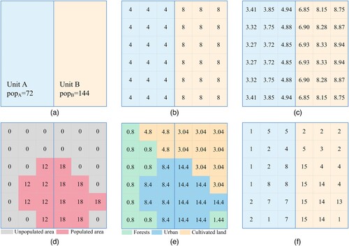
Before disaggregation, a choropleth map is usually used to visualize the population by linking the tabular population with the administrative boundaries (Figure 1a). In recent decades, the two categories of common methods used in population disaggregation are areal interpolation and dasymetric mapping. Population statistical data and administrative boundaries are used as the basic input data for the disaggregation methods. In Figure 1, 72 people in administrative unit A and 144 people in administrative unit B are allocated to grids with a spatial resolution of 100 m according to different population disaggregation methods, which ensures that the original statistical population count is preserved. Figure 1 also illustrates the characteristics of these methods.

Figure 1. Illustrations of the population disaggregation methods. (a) Choropleth map. (b) Areal weighting. (c) Pycnophylactic. (d) Binary dasymetric. (e) Multi-class dasymetric. (f) Intelligent dasymetric.

2.1.1. Areal interpolation

Areal interpolation (Goodchild, Anselin, and Deichmann 1993) can transfer data from one set of objects (i.e. source zones) to another (i.e. target zones) based on the spatial relationship between the two sets of areas. Some researchers have systematically summarized areal interpolation methods from different perspectives. According to whether ancillary data are used, Wu, Qiu, and Wang (2005) divided areal interpolation into two categories: areal interpolation without ancillary information and areal interpolation with ancillary information. Fisher and Langford (1995) grouped areal interpolation into three categories: cartographic, regression and surface method. Lam (1983) divided areal interpolation into two categories according to whether or not the statistically variable values are consistent during the transformation process from source to target zones: volume-preserving (e.g. area-based areal interpolation) and non-volume-preserving (e.g. point-based areal interpolation). This paper mainly introduced the widely used and recognized areal interpolation method in the process of population disaggregation, namely, area-based areal interpolation, which uses the source region itself as the operation unit and maintains the volume-preserving property. For area-based areal interpolation, there are two classical and fundamental methods: areal weighting and pycnophylactic interpolation. Most of the other area-based areal interpolation methods used during the population disaggregation process are based on their improvement (Schroeder 2017).

Areal weighting method (Goodchild and Lam 1980; Goodchild, Anselin, and Deichmann 1993), also known as proportional reallocation, is the most fundamental method in area-based areal interpolation. Given that the population is evenly distributed in each source zone (i.e. administrative unit) (Figure 1b), the population can be allocated according to the overlapping area of the target zone (i.e. a grid) and the source zone. The accuracy of the results increases as the resolution of the basic input data used increases (Hallisey et al. 2017). Limited by this assumption, this method only realizes the conversion of population data from vector administrative areas to grids and cannot express local differences. The advantage of the areal weighting method is that it is easy to operate and has high calculation efficiency, without the need for any ancillary data. Therefore, the population spatial distribution data produced based on this method can be used with other geographic information to study scientific problems without worrying about endogeneity.

Pycnophylactic interpolation (Tobler 1979) is an extension of the areal weighting method. The method assumes that the population of an area tends to be similar to the population of nearby areas. Considering the influence of adjacent areas, a smooth function is applied to the target zone, and the weighted average of its nearest neighbors is used to iteratively smooth the population values in the grids. In each iteration, the total population of the target zones is adjusted to ensure the same population count as the source zone. Finally, a smooth and continuous population surface is produced. This method can effectively address the problem that population values suddenly jump at the edges of the source zone in the area weighting method (Figure 1c, shows the result of using this method after 20 iterations). It should be noted that large changes in population at the edges of the source zone would affect the accuracy of the interpolation. When a high-density population area is adjacent to a sparsely populated area, smoothing will allocate almost all the population in the sparse area to be adjacent to the high-density area.

2.1.2. Dasymetric mapping

Dasymetric mapping (Mennis 2009; Petrov 2012), which was named and developed by Semenov-Tian-Shansky (1928) and subsequently popularized by Wright (1936), refers to subdividing the source zone into smaller areas that can reflect the spatial changes in the population based on ancillary data. The population distribution patterns in the small areas are similar or the same. The final step of dasymetric mapping is usually to apply areal interpolation to generate population distribution data at different scales, so this method can also be regarded as an improvement of areal interpolation. In this paper, dasymetric mapping is divided into three categories: binary dasymetric, multi-class dasymetric, and intelligent dasymetric mapping.

Binary dasymetric mapping (Eicher and Brewer 2001; Holt, Lo, and Hodler 2004), which is mask area weighting in nature, uses ancillary data to divide a source zone into two sub-zones, usually populated and unpopulated areas. The unpopulated area is masked out, and all the population is distributed to the populated area (Langford and Unwin 1994) (Figure 1d). The binary method is widely discussed due to its simplicity. However, the zoning process relies heavily on the researcher’s subjectivity to decide which area is populated and which one is not (Fisher and Langford 1996). In addition, according to the level of regional economic development, the source zone can also be divided into urban and rural areas. The population density difference between the two is obvious. The binary dasymetric method can effectively avoid the problem of underestimation of the population in urban areas (i.e. high-value areas) and overestimation of the population in rural areas (i.e. low-value areas). For example, the disaggregated population product GRUMPv1 was generated based on this method (see Section 2.3 for details).

Multi-class dasymetric method (Mennis 2003; Su et al. 2010) divides a source zone into several sub-zones, which can effectively improve the accuracy of population disaggregation. However, it is necessary to divide the sub-zones according to local knowledge and then to estimate the population count (density) of each sub-zone. This method can directly use each land cover class as a sub-zone, and use regression analysis to determine the population density of each class (Langford, Maguire, and Unwin 1991). Finally, the calculated population density of each class is scaled in proportion to ensure volume-preserving properties. Each source zone can also reallocate the population to the sub-zones (or land cover classes) within it according to the percentage that is subjectively selected, and the sum of the percentage values of the population allocated to these sub-zones is 100% (Eicher and Brewer 2001). For example, the population of administrative unit A is assigned to the urban area, cultivated land, and forestland at 70%, 20%, and 10% values, respectively (Figure 1e). The upper threshold of the population density in each sub-zone is set by the limiting variable method (McCleary 1969) to ensure accurate percentage assignments. Refining the land cover classification can improve the subdivision level of the sub-zones, to minimize the errors caused by the differences between sub-zones. However, with the improvement at the subdivision level, the level of difficulty increases.

Intelligent dasymetric (Mennis and Hultgren 2006; Schroeder 2017) is a more complex modeling method that supports a variety of methods, such as empirical sampling (Mennis 2003), pre-defined population density statistics (Eicher and Brewer 2001), regression (Langford, Maguire, and Unwin 1991; Langford 2006), and machine learning (Gregory 2002; Stevens et al. 2015; Šimbera 2020). It is worth mentioning that deep learning methods can extract highly abstract features, and their non-linear expression abilities are better than traditional machine learning methods in many fields. At present, deep learning methods have been used to disaggregate the population, and their effectiveness has been demonstrated (Gervasoni et al. 2018; Monteiro et al. 2019). Intelligent dasymetric methods define and optimize the relationship (i.e. weighting factors) between the population data and ancillary data that can fully represent natural and economic factors affecting the population distribution, and in the subsequent step, the population of the source zone is dasymetrically allocated (Figure 1f) (Nagle et al. 2014). With the improvement of data processing efficiency, this method gradually evolves towards intelligentization and automation. However, due to the use of multiple variables, the complexity of the model is increased, and redundant information may be generated. Before modeling, it is necessary to use correlation analysis to select appropriate indicators of the population spatial distribution as ancillary data. It should be noted that different scales of the source zone have an impact on the selection of population distribution indicators (i.e. the ancillary data). For example, by taking a sub-national area as the source zone, the influence of topographic factors is obvious, while when using the county area as the source zone, the topographic factors can be ignored, and the impact of urban infrastructure elements should be considered.

Population spatial disaggregation methods simulate the relationship between the population and ancillary data based on different assumptions, and the relationship is used to allocate the population to the target area as the weight. The setting of the weight scheme is a key step, which directly affects the reliability of the results. In the early days, to simplify the models, regardless of the attractiveness of natural and economic factors to the population, it was assumed that the population was evenly distributed within the source zone, and the overlapping areas of the target and source zones were used as the weights to calculate the population. Two weight values, 0 and 1, are set for binary dasymetric mapping to calculate the population of unpopulated and populated areas, respectively, that is, to allocate all the population to the populated area. However, there may be people in the unpopulated areas; for example, there will still be people living in the cultivated land or forestland. These patches are very small and fragmentary, so it is easy to ignore their existence in image recognition due to the limitations of the image resolution and processing methods. Multi-class dasymetric mapping heuristically or empirically calculates weights, which largely depends on human subjectivity. With the introduction of random forest, genetic evolution, neural networks, and other new methods, intelligent dasymetric mapping can flexibly set parameters to calculate or optimize weights (Azar et al. 2013; Stevens et al. 2015). Due to the subjective initiative of human beings and the complexity of the external environment, many factors affect population settlement. With the support of the ancillary data, various methods analyze and deeply mine the population distribution rules and mechanisms to ensure that the results calculated based on the weights can be close to the actual distribution of the population (Lloyd, Sorichetta, and Tatem 2017). At present, these methods have some limitations. There is no one weighting scheme that can accurately reproduce the real population distribution. The setting of the weighting scheme will inevitably introduce uncertainty to the results. When selecting a disaggregation method, it is necessary to fully consider the attributes of the data and the characteristics of the study area to minimize the uncertainty of the results.

2.2. Ancillary data used for disaggregation modeling

The spatial distribution of the population is driven by environmental and socio-economic factors in the region (Nieves et al. 2017). The former includes altitude, climate, vegetation, etc., and the latter includes land use, roads, etc. With the improvement of the technology for acquiring geospatial information, it is easy to obtain and capture the data about these factors as auxiliary data for disaggregation modeling to improve the level of details and accuracy. In this paper, frequently used ancillary data are divided into four categories: land cover, nighttime lights, infrastructures, and environmental factors.

2.2.1. Land cover

Land cover is the product of the interaction between humans and nature and is a direct reflection of the spatial distribution of human activities (Meyer and Turner 1992). Tian et al. (2005) and Gallego (2010) demonstrated the feasibility of simulating the spatial distribution of the population based on land cover. A variant of land use and land cover, impervious surface, is also a commonly used type of ancillary data, which has a role similar to that of land cover (Palacios-Lopez et al. 2019; Palacios-Lopez et al. 2021). In large-scale studies, the total population can be allocated according to the correlation between population counts and classes of land cover or the overlapping areas between each land cover class and its target grid. Some classes of land cover, such as water bodies, glaciers, and protected areas, are not suitable for human habitation. They are used as masks to reduce errors in the process of population disaggregation (Hyman et al. 2004). The classification number and accuracy of land cover determine the reliability and scale of the resulting population distribution (Linard, Gilbert, and Tatem 2011).

The development of remote sensing and image processing technologies provides an opportunity to refine land cover so that detailed residential area data can be obtained, such as the Global Human Settlement Layer (GHLS) (Corbane et al. 2017), the Global Urban Footprint (GUF) (Esch et al. 2013), or even the information of individual buildings (e.g. footprint, height, number of floors, and type) (Sridharan and Qiu 2013). For example, Huang et al. (2021a) disaggregated US census records into 100 m grids based on Microsoft building footprints. Ural, Hussain, and Shan (2011) and Lwin and Murayama (2009) used the three-dimensional information of buildings to map the population at the building scale. Dong, Ramesh, and Nepali (2010) employed LiDAR, Landsat TM and parcel data to extract the building area, volume and count to spatialize the population for Denton, USA.

2.2.2. Nighttime lights

Nighttime lights can sensitively capture and record human activities and are a good proxy for population spatial disaggregation (Archila Bustos, Hall, and Andersson 2015; Kumar et al. 2019). A significant correlation between nighttime lights and population counts has been demonstrated in many countries and regions (Elvidge et al. 1997; Sutton et al. 1997; Zhuo et al. 2009) and is often used as the weighting factor for modeling. However, it should be noted that nighttime lights are mainly affected by economic activities, and the effect of light is not obvious in less developed areas such as North Korea (Levin et al. 2020). Therefore, the social, economic, cultural, and even religious background of the study area should be taken into account when modeling. The intensity, frequency, and location of nighttime lights can be used to extract areas where people may live (Zhou et al. 2014) and can also be used to eliminate vacant buildings in the land cover (Wang, Fan, and Wang 2019) so that the residential area data can be close to the real living situation of humans. Due to the inherent characteristics of the sensors and the limitation of spatial resolution, nighttime lights often overestimate the true extent of the urban area and cannot detect the small residential areas in rural areas and surroundings (Elvidge et al. 2001). To solve these problems, the current trend is to combine nighttime lights and other geospatial data to achieve population spatialization (Briggs et al. 2007).

2.2.3. Infrastructures

Infrastructure is the carrier of human activities, which can attract people to settle down. There are some commonly used ancillary data, such as transportation networks (including roads, railroads, navigable waterways, and airports), health facility locations, schools, police stations, etc. Roads are particularly significant in modeling because roads play an important role in linking social, economic, cultural, and other activities in regions. The density of infrastructure features and the distance and time cost from any location to infrastructures (i.e. accessibility) can be calculated to characterize their influence on the population spatial distribution. Yue et al. (2005), Ye et al. (2019), and Yao et al. (2017) have all attempted to use various infrastructure data for spatial disaggregation with satisfactory results. The UNEP/GRID population product calculated the accessibility of roads and urban centers to simulate population distribution (Hyman et al. 2004). When using infrastructure as ancillary data for population spatial disaggregation, it is necessary to consider how its level (e.g. highways and paths, hospitals and clinics) and corresponding service coverage affect the ability to attract people to live, that is, how to weight different levels of infrastructure.

Volunteered Geographic Information (VGI) can be considered a sub-category of infrastructure data, which has the characteristics of low cost and fast update and has potential in population spatial disaggregation (Aubrecht, Ungar, and Freire 2011). There are two main sources, namely, OpenStreetMap (OSM) and Points of Interest (POI). The former collects vector-based data such as streets and buildings, which are used to simulate the spatial distribution of the population (Rosina, Hurbánek, and Cebecauer 2017). The latter, whose density and agglomeration trend can represent human living conditions and behaviors, consists of the location and attribute information of all types of urban facilities (Yang et al. 2019). Other VGI data that can record the location of people are also increasingly being used for population disaggregation, such as taxi trajectory data (Yu et al. 2019), traffic smart cards (Ma et al. 2017), mobile phones (Chen et al. 2018), and Twitter (Lin and Cromley 2015) from social media data. Before modeling, it is necessary to consider the integrity, coverage and logical consistency of VGI data, and judge whether the data are valuable as ancillary data, and then perform some pre-processing work.

2.2.4. Environmental factors

The physical environment has a significant impact on the population distribution on a large scale. In most cases, people prefer to settle in areas with suitable climates and gentle terrain (Small and Cohen 2004). Commonly used ancillary data include climate (i.e. temperature and precipitation), elevation, slope, Net Primary Productivity (NPP), etc. Climate influences soil fertility, agricultural development and industrial structure, so it may be the driving factor of population living patterns (Le Blanc and Perez 2008). Elevation usually plays an obvious role in the vertical distribution of the population to a certain extent (Cohen and Small 1998), and thus it is an important indicator reflecting the population distribution potential. Generally, with increasing elevation, the population count decreases. In addition to elevation, the effects of slope, aspect, and relief degree of the land surface on population settlement should also be considered. NPP is useful for population disaggregation studies because population counts are spatially correlated to the NPP (Luck 2007). Yue et al. (2005) used vegetation NPP as one of the input data of the grid generation method to simulate the spatial distribution of the population in China. Lloyd et al. (2019) and Stevens et al. (2015) used temperature and precipitation as the input layer of the population disaggregation model to generate population distribution data.

2.3. Disaggregated population products

In recent years, the disaggregated population products that are created using the above methods and factors have increased significantly and become increasingly popular in various research fields. For detailed population product information, please refer to the review by Leyk et al. (2019). Here, representative products are briefly summarized with respect to methods, ancillary data used, coverage, spatial and temporal resolution, and limitations to help researchers understand and select the products that are most suitable for their intended uses. The characteristics of these products are summarized in Table 1. There are two population concepts presented in this table: the residential population and ambient population. The former refers to those people that who live in a residential area most of the time, and the latter refers to those people that may be present in an area due to local cultural, economic, or social factors over a short period of time (this is the average over 24 h).

Table 1. Disaggregated population products and their main characteristics.

Dataset	Coverage	Resolution	Year(s) represented	Method	Ancillary data used	Population concept	Distribution policy	Source
Gridded Population of the World (GPWv4) (Doxsey-Whitfield et al. 2015)	Global	30 arc-seconds (∼1 km)	2000, 2005, 2010, 2015, 2020	Areal weighting	None	Residential	Open	https://sedac.ciesin.columbia.edu/data/collection/gpw-v4
Global Rural-Urban Mapping Project, Version 1 (GRUMPv1) (Balk et al. 2005; Salvatore et al. 2005; Balk et al. 2006 )	Global	30 arc-seconds (∼1 km)	1990, 1995, 2000	Binary dasymetric mapping	Nighttime lights, settlement points	Residential	Open	https://sedac.ciesin.columbia.edu/data/collection/grump-v1
LandScan Global Population (Dobson et al. 2000; Bhaduri et al. 2007)	Global	30 arc-seconds (∼1 km)	1998, annual release from 2000 to 2019	Multivariate dasymetric mappingc(or smart interpolation)	Nighttime lights, roads, slope, elevation, land cover, urban boundaries, high resolution imagery	Ambient	Free for research/ commercial use at cost	https://landscan.ornl.gov/
WorldPop (Tatem 2017)	Africa, Asia, Central and South America	3 arc-seconds (∼100 m)	2000–2020	Semi-automated dasymetric mapping	Settlement, roads, land cover, urban areas, nighttime lights, infrastructure, climate, vegetation, elevation, slope, protected areas, water bodies, building maps	Residential	Open	http://www.worldpop.org/
Global Human Settlement Layer-Population (GHS-POP) (Freire et al. 2016; Freire et al. 2020)	Global	9 arc-seconds (250 m) and 30 arc-seconds (1 km)	1975, 1990, 2000, 2015	Dasymetric mapping	Global Human Settlement Layer – built-up areas (GHS-BUILT), GPWv4	Residential	Open	https://ghsl.jrc.ec.europa.eu/ghs_pop2019.php
UNEP/GRID-Sioux Falls (Deichmann 1996b; Hyman et al. 2004; Nelson 2004)	Africa, Asia and Latin America and Caribbean	2.5 arc-minutes (∼5 km)	1960-2000, decade interval (Africa, Asia and Latin America); 1995 (Asia)	Areal weighting	Transportation network, urban centers, location and size	Residential	Open	https://na.unep.net/siouxfalls/datasets/datalist.php
World Population Estimate (WPE) (Frye et al. 2018)	Global	150 m (2016), 250 m (earlier)	2013, 2015, and 2016	Dasymetric mapping	Land cover, roads, water bodies, cities or urban areas	Residential	Commercial / Free to ArcGIS Users	https://livingatlas.arcgis.com/en/browse/#d=2&q=World%20Population%20Estimate
High Resolution Settlement Layer (HRSL) (Tiecke et al. 2017)	Countries	1 arc-second (∼30   m)	2015	Binary dasymetric mapping	Digital Globe 0.5 m imagery	Residential	Open	https://www.ciesin.columbia.edu/data/hrsl/
OpenPopGrid (Murdock et al. 2015)	United Kingdom	10 m	2011	Binary dasymetric mapping	Postcode centroids, building footprints	Residential	Open	http://openpopgrid.geodata.soton.ac.uk/
PopGrid (Huang et al. 2021a)	the Contiguous United States	100 m	between 2013 and 2017	Dasymetric mapping	Microsoft building footprints, OSM	Residential	Open	https://doi.org/10.7910/DVN/DLGP7Y

GPWv4 does not use ancillary data during the generation process. Therefore, this product does not need to worry about endogeneity and can be used with geospatial data in subsequent analyses without restrictions. GRUMPv1, a research-oriented product, provides urban-rural populations for understanding poverty issues. Different from other datasets, LandScan uses an ambient population rather than a residential population. It can be capable of capturing human activities during the day to provide services for emergencies. Because input data sets are constantly improved, which leads to changes in population distribution, cell-by-cell comparison among Landscan products of annual time series should be avoided. It is worth noting that although WorldPop is introduced as a disaggregated population product; this aggregation method is used for specific countries or regions where censuses are lacking or inaccurate. WorldPop uses a large amount of auxiliary data to develop high-resolution population data, which is suitable for fine-scale applications. GHS-POP and UNEP/GRID-Sioux Falls are multi-temporal population data products that can study how the population has changed over time in recent decades. The resolution of UNEP/GRID-Sioux Falls may be too coarse for applications at the sub-national level. The aforementioned products with large coverage and medium spatial resolution values play an important role in SDGs assessments at the global and continental levels. With the increasing demand for rich details of population spatial distribution, some population datasets or products with high spatial resolution have been produced in recent years, which is beneficial to support the evaluation of population-related SDGs at the national and regional levels. Table 1 lists three open high-resolution products, namely, HRSL, OpenPopGrid, and PopGrid, of which OpenPopGrid has a resolution of 10 m.

3. Applications supporting SDGs assessment

To promote the coordinated development of economic growth, social inclusion and a beautiful environment worldwide, in September 2015, the United Nations proposed 17 Sustainable Development Goals (SDGs) (UN 2015) and 169 targets. In 2017, the Inter-Agency and Expert Group on SDG Indicators (IAEG-SDGs) established by the United Nations proposed a Global Indicator Framework for SDGs, which includes 244 indicators to guide countries or regions to carry out quantitative assessment, regular monitoring and regular reporting of SDGs. The framework is reviewed and improved annually. In 2020, 247 indicators are listed in the framework, but 12 of these are repeatedly attributed to two or three targets, so the actual total number of indicators is 231 (the expressions below are all in this context) (UN 2020a). According to the development level of the calculation methods and the availability of data, SDG indicators are divided into three levels (UN 2020b). Tier I indicators have mature calculation methods and easy access to data. Tier II indicators have mature calculation methods, but data are often missing. Tier III indicators lack recognized calculation methods and effective data. As of July 17, 2020, the updated tier classification includes 123 Tier I indicators, 106 Tier II indicators, and two indicators with multiple tiers (UN 2020b), as shown in Table 2.

Table 2. SDGs Global Indicator Framework (as of 2020) and indicators that can be supported by disaggregated population data.

Note: Blue signifies indicators directly supporting SDGs assessment and belonging to Tier I, and the use of population spatial disaggregation data can optimize the calculation results derived from statistical data. Yellow and orange both signify that direct support and that the indicators belong to Tier II. In the case of a lack of data, the former can realize the calculation of indicators by integrating population disaggregation data and other data, while the latter can play an important role in SDGs assessment only when the metadata required for the indicator calculation are available. Green means indirect support. Grey signifies that the indicators have nothing to do with the disaggregated population data. The symbol in the upper right corner of the indicator indicates that this indicator is repeated. For example, indicators 7.b.1 and 12.a.1 have the same symbol, ▴, indicating that they are the same and repeat. All repeat indicators: 1.5.1/11.5.1/13.1.1, 1.5.3/11.b.1/13.1.2, 1.5.4/11.b.2/13.1.3, 4.7.1/12.8.1/13.3.1, 7.b.1/12.a.1, 8.4.1/12.2.1, 8.4.2/12.2.2, 10.3.1/16.b.1, 10.6.1/16.8.1, 13.2.1/13.b.1, 15.7.1/15.c.1, 15.a.1/15.b.1.

Approximately half of the SDG indicators are related to the population and its geographical location. The SDGs emphasize ‘leave no one behind’, which means that we need to pay attention to not only how many people live in the administrative units but also where they live. Due to the importance of improving the spatial heterogeneity of the indicators, there is an increasing need for reliable and spatially detailed population data to assess and monitor the UN SDGs, to identify problems in a timely manner and to formulate improvement measures.

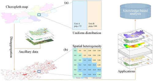
Before disaggregation, a choropleth map is usually used to visualize the population by linking the tabular population with administrative boundaries. As shown in Figure 2a, the population is uniformly distributed within the region of interest (blue rectangle). The disaggregated population data can provide rich details of population distributions beyond administrative boundaries (Figure 2b) and can be flexibly integrated with multi-source geospatial data. Therefore, it can effectively support the calculation and assessment of population-related SDG indicators and provide knowledge-based services for decision-makers and the public.

Figure 2. Illustration of disaggregated population data applications.

According to preliminary statistics (UN World Data Forum 2018), disaggregated population data can directly support the calculation and evaluation of 45 indicators. Among these, 38 indicators can be calculated according to the population statistical data. In addition, the evaluation results of these indicators can be optimized after the use of disaggregated population data and the numerical value become more accurate, which can break through the restriction of administrative units in space. Twenty-nine of these indicators belong to Tier I and are marked in blue in Table 2. The calculation methods of these indicators are mature, and the data are available. Nine indicators belong to Tier II, marked in orange in Table 2. Although they have mature calculation methods, the required data are often missing. Only when the metadata required for indicator calculation are available can disaggregated population data play an important role. In addition, the seven indicators belonging to Tier II, marked in yellow in Table 2, are often difficult to monitor. In the absence of metadata, the calculation of such indicators can be achieved by integrating disaggregated population data and the use of other data to track and measure the sustainable progress of the indicators. Disaggregated data can also indirectly support the evaluation and monitoring of the 62 indicators marked in green in Table 2, because they do not participate in the calculation of indicators. According to the population spatial distribution data and other multi-source data related to the indicators, the sustainable progress of the indicators is described and monitored in multiple dimensions and at multiple levels so that the indicators or the corresponding targets can be interpreted in a broad context.

In the following sub-sections, two specific cases are presented.

3.1. Application 1: assessing indicator 3.8.1 at the county level

Deqing County, located in northern Zhejiang Province, China, is a pilot area for evaluating the progress of China’s SDGs (Chen and Li 2018). Qiu et al. (2019) disaggregated the town-level population data into 30 m grids based on the dasymetric mapping method and three-dimensional building information (including building areas and the number of floors). Indicator 3.8.1 (a green mark in Table 2) was selected to discuss the application of population spatial disaggregation in the SDGs assessment. Based on the characteristics of Deqing County, the indicator was revised to ‘coverage of essential health services’ after localization.

Accessibility analysis was used to calculate the time required for the residents to reach the nearest medical facilities, and the result is shown in Figure 3. The areas with good accessibility were concentrated in the middle and on the east side of Deqing. Due to the mountainous area and sparse roads on the west side, accessibility there was poor. Based on the accessibility results, the difference between using population statistical data and disaggregated population data to quantify and evaluate SDG indicators was analyzed.

Figure 3. Accessibility of health centers in Deqing County (from Qiu et al. 2019).

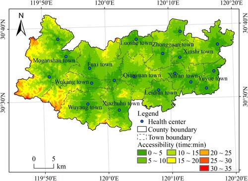
As shown in Table 3, the assessment results based on population statistical data showed that 7.93% of residents needed to spend more than 15 min to reach the nearest health centers. The areas with accessibility values greater than 15 min were located in the western mountainous area. There were also urban-rural differences in the level of medical services in Deqing County. According to the assessment results of disaggregated population data, only 1.06% of residents need to spend more than 15 min. Through high-resolution remote sensing images, it was identified that the area with an accessibility time of 25–35 min was located in a forest area and that it was uninhabited. In fact, the accessibility of health centers in Deqing County was good, and the spatial distribution of medical resources was reasonable. The evaluation results based on the disaggregated population data are more accurate and reliable than those calculated based on the original statistical data.

Table 3. Percentage and cumulative percentage of the population who could reach a health center within each time interval based on population statistical data and disaggregated population data (cite from Qiu et al. 2019).

Time (min)	Population statistical data		Disaggregated population data
	Percentage (Health Center)	Cumulative Percentage (Health Center)	Percentage (Health Center)	Cumulative Percentage (Health Center)
0–5	23.32	23.32	46.16	46.16
5–10	49.42	72.74	44.10	90.26
10–15	19.34	92.07	8.68	98.94
15–20	5.66	97.73	0.96	99.90
20–25	1.90	99.63	0.10	100
25–30	0.33	99.97
30–35	0.03	100

3.2. Application 2: assessing indicator 11.3.1 on a global level

In Table 2, SDG indicator 11.3.1, the ratio of the land consumption rate to the population growth rate, i.e. the land use efficiency (LUE), is marked in yellow. This indicator is a Tier II indicator. In the absence of metadata, this indicator can be calculated by integrating disaggregated population data and other data. Schiavina et al. (2019) demonstrated the feasibility of the assessment of indicator 11.3.1 on a global level based on the GHS-POP product. The evaluation results could facilitate the understanding of the interaction between land consumption and population changes.

The GHS-POP data present population counts within each grid at 250 m resolution (or 1 km, aggregated from 250 m) in world Mollweide equal-area projections for 1975, 1990, 2000, and 2015. The spatial population distribution data can replace the population statistical data as the denominator of the indicator calculation formula to directly calculate the indicator and improve the accuracy of ratio-based indicator evaluation (Tatem 2014). The research of Schiavina et al. (2019) provided an opportunity to upgrade indicator 11.3.1 from the Tier II classification and showed the value of using disaggregated population data in monitoring the progress of the SDGs.

3.3. Summary

These two examples show that spatially accurate and detailed population distribution data are essential for tracking progress on the SDGs and scientifically allocating resources. At present, disaggregated population data sets, including well-known products and locally produced products, have been widely considered and applied in the quantification and evaluation of SDGs. Figure 4 shows the use frequency of disaggregated population data with different spatial resolutions in indicator evaluation applications at global, national, and regional levels. Disaggregated population data were frequently used for the evaluation of the indicators of goals 1 – poverty (Calka, Da Costa, and Bielecka 2017; Andrew et al. 2019; Freire et al. 2019; Smith et al. 2019), 3 – health care services (Snow et al. 2005; Linard and Tatem 2012; James et al. 2018; Juran et al. 2018), 4 – education (Qiu et al. 2019), 6 – safe drinking water (Yu et al. 2017), 7 – electricity (Doll and Pachauri 2010), 9 – infrastructure (Wu and Murray 2005; Andres, Boden, and Higdon 2016; Tiecke 2016; Gaughan et al. 2019), 11 – housing (Ehrlich et al. 2018; Grippa et al. 2019; Michanowicz et al. 2019), and 16 – peace (Corbane et al. 2016). Buffer zones, accessibility results, disease risk maps, etc. are overlaid on population distribution data to quantify the population of the region of interest. This method is often used to evaluate indicators 3.3.3, 3.8.1, 9.1.1, 11.1.1, etc. Disaggregated population data can replace statistical population data as input data for some models (e.g. disaster assessment model), which improves the spatial heterogeneity of the assessment results and supports the measurement and evaluation of indicators 1.5.1, 3.2.1, 3.2.2, etc.

Figure 4. The frequency of use of disaggregated population data with different spatial resolutions in indicator evaluation applications at global, national, and regional levels.

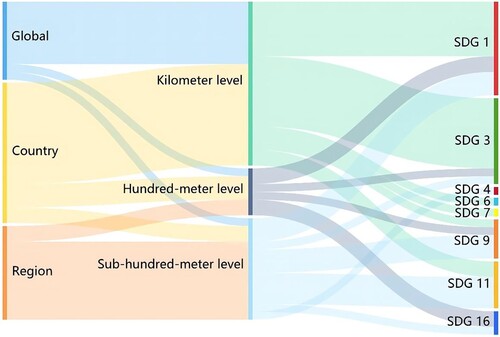
Figure 4 shows that population data with low spatial resolution are not necessarily used in large-scale study areas, and population data with high spatial resolution are not necessarily used in small-scale study areas. There is no necessary relationship between the two. The design and use of population data sets depend on the data, the characteristics of the study area, and the research background. Well-known population products have the characteristics of wide coverage and can provide application consistency. However, the spatial resolution is generally low, which limits the application scenarios. Locally produced population data usually have high resolution, which can show the characteristics of the population spatial distribution in detail. However, its production process is not easy to utilize in other areas. There is an inevitable uncertainty in disaggregated population data. There are uncertainties in the selection of basic input data and ancillary data, the selection of expressing scale for population disaggregated results, and the determination of population weight schemes, and these uncertainties will disseminate to the indicator assessment results without hindrance (Nagle et al. 2014). The possible sources of uncertainty are discussed in Section 4.1 to understand where future work is needed.

4. Discussion

4.1. Challenges with spatial disaggregation

Overall, the population disaggregation methods are gradually becoming more intelligent, and the ancillary data used for modeling are gradually diversifying and developing towards three dimensions. These advances have improved the accuracy and level of details of the population spatial disaggregation results. Moreover, the ability of the population spatial distribution data to support the calculation and evaluation of the SDG indicators on a fine scale has been continuously expanded and developed. At the same time, due to the complexity of the population distribution rules, the limitations of various methods, and the uncertainties introduced in the modeling process, there are still some issues and challenges in the current research.

4.1.1. Available and high-quality input data for modeling

For the top-down population gridding methods, the accuracy of the results depends largely on the quality of the input data (Hay et al. 2005). The lowest level of population and administrative boundaries are not always available due to confidentiality. There are great differences among countries in terms of census data quality, the number and scale of enumeration units, and the frequency of data collection. In low-income countries or regions, census data may be frequently misreported (Wak et al. 2017). The time mismatch between population data, administrative boundaries, and ancillary data, which is limited by the difficulty of data acquisition and update frequency, brings some uncertainties to the results of population disaggregation (Nagle et al. 2014; Leyk et al. 2019). In general, if the administrative boundary corresponding to the census data is spatially accurate, the lower the administrative boundary level is, the smaller the source area is, and the spatial size tends to be close to that of the target area (Doxsey-Whitfield et al. 2015). Then the results will be close to the real population distribution and thus become more reliable. Therefore, obtaining census data for low-level administrative units is the priority of population spatial disaggregation research (Hay et al. 2005), which can effectively reduce the inherent uncertainty brought by the use of census data as the basic input data to the model. Many countries usually conduct national or large-scale censuses every 10 years or more, which consumes considerable time and resources. During this period, a census may be put on hold by factors such as war or disaster. Some population-related studies require not only population distribution data for a certain period but also long-term series data to provide support for its dynamic evolution process. It is necessary to extrapolate from the census year to the target year based on the population growth rate, but the farther the target year is from the census year, the lower the accuracy. Administrative boundaries may change over time, and changes in the boundaries need to be coordinated.

The rapid development of information technology provides an opportunity to efficiently provide high-quality and high-resolution population data. For example, the United States tried to use GIS methods and cloud computing (Laaribi and Peters 2019) to provide geo-referenced censuses, which can effectively improve data quality and distinguish urban and rural populations. China used electronic ways to conduct the 2020 census, such as APP and QR codes, to provide accurate population information to support economic and development planning (National Bureau of Statistics 2020). Under the condition of complying with the user privacy agreement, it is convenient for release to the public. Census records contain the long-term resident population in the area. The geo-referenced data commonly used in bottom-up methods, such as call detail records and Twitter, can be updated quickly and identify the location of individuals during the day, which is a useful supplement to traditional census data. Combining the resident population recorded in the census data with the daytime population will expand the SDGs assessment application of population disaggregation results, especially to guide the rapid response to hazards (Ahola et al. 2007).

In addition, the ancillary data used in modeling may have quality problems due to their own characteristics or production conditions, such as the ‘blooming effect’ of nighttime lights, incorrect topological relationships of the vector elements (e.g. roads) and imagery covered by clouds, which will change the uncertainty level of the results. Efforts need to be made in data processing to reduce the uncertainty.

The rapid development of remote sensing technology has provided rich, high resolution spatial–temporal ground information with large coverage (Burke et al. 2021). Deep learning has a strong ability to extract rich information from remote sensing images (Allen et al. 2021) and can establish a mapping relationship with high robustness between images and population. Remote sensing would be the only input source of population spatialization (Huang et al. 2021b), and it will greatly facilitate population mapping and SDGs assessment for countries or regions lacking statistical population data. The combination of remote sensing and deep learning provides a new direction for population spatialization.

4.1.2. Optimal scale of the disaggregated population

Scale is an old scientific problem in the field of geosciences. With the change in observation scale, the information about population distribution phenomena will also change. The smallest distinguishable part of the disaggregated population result, that is, the grid size, can be understood as the measurement scale or resolution. In fact, the observation scale and measurement scale often do not match (Lam and Quattrochi 1992). Spatial data of population distribution are mainly constructed on a single grid size varying from meters to kilometers. Coarse granularity data have good stability but cannot capture differences in the population spatial distribution in detail, while fine granularity data make up for the details of the space but tend to fall into the local area and easily ignore the general law of the study area (Ge et al. 2019). There is also evidence indicating that the refinement of the scale of population disaggregation data does not necessarily mean the improvement of the accuracy of the actual results (Scholz, Andorfer, and Mittlboeck 2013). If the selection of scale is not suitable, the spatial distribution characteristics of the population cannot be effectively depicted, and it will bring uncertainty to the results of population disaggregation and affect the sensitivity of the results (Sémécurbe, Tannier, and Roux 2016; Sinha et al. 2019). Therefore, it is a challenge to select an optimal scale for disaggregated population data. Suitability is a complex problem. For example, for the same geographical context and modeling method, the suitability scales may be different for various application purposes. In future studies, the range of grid size can be determined according to the research objectives, study area, ancillary data, method, accuracy requirement, etc. Then, from the statistical characteristics (Woodcock and Strahler 1987), spatial autocorrelation (Dong et al. 2017), and landscape spatial patterns, the assessment system of grid size suitability of population spatial data can be established to determine the optimal grid size domain and understand the rules of the resulting data changing with scale. It should be noted that when the resolution of the resulting grid is very high, the movement of residents becomes a factor that cannot be ignored. The objective of disaggregation is no longer the residential population but the ambient population.

4.1.3. Error estimation

The performance of the same model for different regions or environmental conditions may be different (Fotheringham, Charlton, and Brunsdon 1996). The error estimation of the disaggregation results is of great significance to judge the practicability of the results and deepen people’s understanding of the spatial structures and settlement patterns (Calka and Bielecka 2019). The ideal method is to count the population of the sample area with the same resolution or higher resolution than the results, but this is not easy to achieve due to time and financial constraints. At present, there are two main methods to describe the accuracy of the results. One method is to compare the census data with the disaggregation results. However, to reduce the uncertainty of the model, many studies directly used the available census data with the highest level of resolution as the input of the model. Another method uses geospatial metrics (e.g. the root mean squared error, coefficient of variations, mean percent error, and relative error) to compare the differences in the spatial structure and spatial correlation between population disaggregation results and existing population products (Sabesan et al. 2007). Although it is difficult to quantify the error of the model itself, this method helps to understand which specific areas are not well modeled and which areas should be focused on. VGI data provide an opportunity to establish a reasonable and operable error estimation system. In future research, we can consider selecting the appropriate area as the sample area, using geo-referenced data, such as mobile phone locations, as supplementary field survey data, analyzing the accuracy of the population disaggregation method, and judging whether it is worthwhile to extend the method to areas with similar or the same environment.

4.1.4. Expression and management of the disaggregated population data

The spatial disaggregation of the population data allocates population statistical data recorded by administrative areas into grids of specific size according to a mathematical model to realize the conversion of statistical units from administrative units to grids. The disaggregated population data need to meet the multi-scale expression to support the measurement and evaluation of the SDG indicators at different levels in the global scope and then excavate the sustainable status of the indicators from multiple dimensions to help governments at all levels formulate targeted intervention measures. Generally, population data are disaggregated to a latitude-longitude grid, which cannot guarantee the same area of grid cells, leading to the deformation of the grid (Tobler and Chen 1986), and the grid deformation degree will be increased with the increase of the latitude from the equator to the poles. Although the deformation problem has little impact on the spatial disaggregation data in local areas, it will greatly reduce the credibility of subsequent results analysis and policy-making when conducting multi-scale spatial analysis of population distribution on a large or global scale. Therefore, the latitude-longitude grid cannot meet the needs of management, updating and application of multi-scale population spatial disaggregation data.

The equal-area Discrete Global Grid System (DGGS) (Sahr, White, and Kimerling 2003), which is a model that can effectively manage massive geospatial data, recursively divides the sphere (or the Earth’s surface) into grids with equal areas and a multi-resolution hierarchical structure and uses the address code corresponding to each grid instead of the geographic coordinates to operate on the sphere. Because grids of different levels not only record the location information but also record the scale and accuracy information, these grids have the potential to process multi-scale spatial data. The equal-area DGGS provides an effective method to realize the continuous digital expression of large-scale population spatial disaggregation data and improve the accuracy of spatial statistical analysis. Equal-area DGGSs have been successfully applied in some fields, such as climate analysis (Randall et al. 2002), ocean simulation (Ii and Xiao 2010), and environmental monitoring (Karssenberg and Jong 2005), but the application of equal-area DGGSs to SDGs monitoring and evaluation systems based on population spatial disaggregation is still a challenge. On the one hand, the operations of grid subdivision, coding and indexing are complex, and there is no available software or tool to directly construct the spatial expression and management framework of multi-scale data based on equal-area grids. Researchers who study the spatial disaggregation of populations usually lack or are not familiar with the knowledge of equal-area DGGSs. On the other hand, the geometric shape of the grids and the geometric relationship between the grids have changed due to the spherical characteristics, which makes the geometric processing of the grids difficult. At present, there is no population spatial disaggregation method suitable for equal-area DGGSs. How to use equal-area DGGSs to realize the expression and management of disaggregated population data has not been experimentally studied.

4.2. Disaggregated population as an essential SDG variable

SDGs include three dimensions (society, economy, and environment) as well as many themes such as climate, ocean, and education. They have complex giant systems and significant temporal and spatial characteristics, which bring challenges to the construction of efficient and standardized SDGs monitoring and evaluation systems. The Essential Variable (EV) is the minimum number of variables to determine the state and development of the system (Bombelli et al. 2015), which can effectively reduce the monitoring burden, avoid unnecessary redundancy, and provide the possibility to construct an ideal system and realize complex system observations. EVs have been developed in the fields of climate (Bojinski et al. 2014), biodiversity (Pereira et al. 2013), ocean (Lindstrom et al. 2012), water (Lawford 2014), air quality (Shelestov et al. 2020), renewable energy (Ranchin et al. 2020), and ecosystems (Bombelli et al. 2015) to maximize the use of data and coordination systems. EVs can not only focus the monitoring system on more effective observations but also help capture the key dimensions of the system. Reyers et al. (2017) and Stafford-Smith et al. (2017) suggested that according to the content and demand of SDGs monitoring, a set of EVs or ESDGVs reflecting the main characteristics and changes of SDGs should be defined and extracted as the objective of continuous monitoring to construct an efficient and unified SDGs monitoring system.

Learning from some existing EVs, such as Essential Climate Variables (ECVs) and Essential Ocean Variables (EOVs), we can thoroughly analyze the spatial–temporal characteristics of SDGs and the impact of population as a social subject on the environment and economy and the feedback effect and propose the basic idea of SDGs assessment based on the spatial distribution of the population. The criteria for selecting EVs are considered, and the requirements of SDGs monitoring on its connotation, scale (resolution), accuracy, etc. are analyzed to identify the potential of the disaggregated population as the EV for SDGs spatial monitoring, which provides opportunities for building a standardized and unified SDGs monitoring system and realizing scientific and efficient monitoring and evaluation. The criteria for selecting EVs (Bojinski et al. 2014) include relevance, feasibility, and cost effectiveness.

Relevance means that the variable is essential for evaluating and analyzing the status and changes of population-related indicators. Approximately half of the SDG indicators are related to population and its geographical location. Population distribution data can quantify the spatial scope of human activities on a global scale to measure the impact of human activities on the environment, economy, and society. Population spatial distribution and change play a key role in reflecting the distribution characteristics and spatial and temporal effects of SDGs. Defining disaggregated population as the ESDGV provides an opportunity to reduce the observation duplication between SDG indicators, meet the flexibility of dynamic and multi-scale monitoring, and build an efficient evaluation system (Reyers et al. 2017).

In this paper, the importance of disaggregated population data as an EV to the whole SDG monitoring system is judged by the way the data directly or indirectly support SDGs calculation and evaluation. However, it must be noted that there are limitations in the calculation methods of some indicators given by IAEG-SDGs. For example, the existing formula of indicator 11.3.1 only evaluates the relationship between the land consumption rate and population growth rate from an economic perspective, without considering its impact on society and environment (Choi et al. 2016). The SDGs system emphasizes the coordinated development of the economy, social inclusion, and a beautiful environment. It also emphasizes the role of human beings in environmental, economic and social development aspects, especially the inclusion of poor and vulnerable groups. Therefore, in future research, it is necessary to fully understand the concept of indicators based on the social, economic, and environmental dimensions, sort out the multi-level relationships among the goals, targets, indicators, spatio-temporal population information, and basic observation data to form a multi-level association model, improve and perfect the evaluation method of indicators, and mine more indicators that can be calculated or explained using essential disaggregated population variables.

Feasibility means that it is technically feasible to observe or derive variables on a global scale based on scientifically understood and proven methods. The methods, data, products, and advantages and disadvantages of obtaining geo-referenced population data have been described in detail. Therefore, it is technically easy to extract disaggregated population data as an Essential Variable for SDGs according to existing methods and data. In the context of rapid changes in social and economic activities brought up by rapid urbanization and population expansion, natural disaster risks and the refinement of social management also put forward new requirements for the spatial–temporal resolution of population distribution data. In the actual research process, the spatial–temporal resolution is mainly determined according to the research object, scope, data source, method, and so on. VGI data can capture socioeconomic characteristics well, which makes it possible to obtain long-term series and high-precision population movement data. Combining VGI data with census data can be used to create easily updated real-time population estimation data sets. However, there are still some problems in using VGI data to supplement or replace the statistical population data released by the national authorities, such as the large amount of data, their unstable quality, redundancy, incompleteness, and lack of unified norms. Therefore, more efforts should be made to mine the value of VGI data in obtaining the disaggregated population as an Essential Variable for SDGs. In recent years, people have become increasingly interested in studying the quality evaluation and integration of multi-source heterogeneous information, such as revealing the complex relationships and transformation rules among various types, scales, time, semantics, and reference systems, to screen useful data with high reliability to help calculate disaggregated population data as EVs (Bordogna et al. 2014).

Based on disaggregated population variables and multi-source spatio-temporal data, research on SDGs monitoring and knowledge services can be carried out. On the one hand, we need to develop SDGs indicator calculation methods based on disaggregated population variables. Forty-five indicators can be calculated directly using the disaggregated population variable or comprehensively using statistical data and the variable. For the 62 indicators that can be indirectly supported by the disaggregated population data, it is necessary to design special algorithms or models to extract the relevant spatial parameters, such as density, relationship, accessibility, and coverage, to accomplish the calculations and evaluations of the indicators (Liverman 2018). On the other hand, due to the observation requirements of the disaggregated population variables (such as spatio-temporal resolution, frequency, and accuracy), the ability to obtain the variables, and the meaning of indicators, the applicability of the disaggregated population data to support SDGs assessment is different in different contexts. It is necessary to evaluate the applicability and usefulness of the disaggregated population data as an EV in providing information for various policy frameworks such as SDGs. At present, studies have mainly focused on the acquisition of the disaggregated population variables, and the evaluation of the applicability of these variables has been less. It can be considered based on the observation requirements, measurement capabilities, and their benefits to construct an evaluation system for the applicability of disaggregated population variables serving SDGs to provide the basis for the efficient use of these variables.

Cost effectiveness means that it is affordable to generate and archive data about these variables, which mainly rely on coordinated observation systems that use mature technology, and take advantage where possible of historical data sets. As mentioned in Section 2.2, with the progress of information acquisition technology, in most cases, the data used to extract the disaggregated population variables can be obtained free of charge, meeting the needs of SDGs monitoring and evaluation. Integrating international high-resolution, high-frequency global (or large-region) geospatial data and local data to form new data sets that can improve resolution or accuracy is an effective way to reduce the observation cost. It is also a good choice for countries or regions that lack high-quality data (Selomane et al. 2015). For example, Grippa et al. (2019) combined OSM data and local Very High Resolution (VHR) imagery to accurately extract the location and range of slums to estimate population density. In response to the need to serve SDGs evaluation based on disaggregated population variables, developing spatial data fusion methods is a future research task.

The benefit of disaggregated population data as an EV to serve SDGs can be understood as the degree to which the variable successfully supports the analysis of the status of SDGs, the extraction of knowledge and the realization of knowledge services. To maximize the benefits of disaggregated population data as a variable, it is necessary to consider people’s spatial cognitive habits, extract knowledge about population-related SDGs from the monitoring results, and carry out structured modeling, correlation processing, and visual expression. Evaluators must form a knowledge network of SDGs that is easy to understand and use to provide decision-makers and the public with facts about population information and help them understand where problems or gaps exist (Kanter et al. 2016; Plag and Jules-Plag 2020). One of the key scientific issues is to develop effective methods to visualize the status and trends of SDG indicators and to communicate the results to decision-makers and other users. Li et al. (2020) used the where-when-what system to identify nine scenarios and described the functional requirements and framework for the dynamic and multi-dimensional visualization of SDGs. However, discussion and cases on the visualization of SDGs based on EVs are still rare, which is another research direction in the future.

5. Summary

This paper aims to clarify the concept of disaggregation. We summarize the progress in methodology, ancillary data used for modeling, and disaggregated population products, while emphasizing the role of disaggregated population data in SDG indicator assessment, and discuss the future work from two perspectives: challenges with spatial disaggregation and disaggregated population as an ESDGV.

Population disaggregation methods change from a simple areal weighting method to an intelligent dasymetric mapping that can fully consider natural and social factors. The existing methods are mainly different in two aspects, namely, the type and source of ancillary data and the disaggregation weight scheme (Langford 2006). On the one hand, the ancillary data used for modeling are developing towards multiple sources and new types, from single land use to the integration of multiple geographic information. Due to the diversity of data, it is necessary to select appropriate indicators of population spatial distribution as ancillary data to avoid information redundancy based on correlation analysis. On the other hand, based on regression, machine learning and other methods, the relationship between the population and ancillary data is derived to determine the weights to dasymetrically distribute the statistical population. Because the spatial distribution mechanism of the population is not yet clear and the indicator factors are complex and diverse, therefore it is not easy to infer which model has more universal significance (Langford 2007). As high-resolution and LIDAR imagery becomes increasingly accessible, it is easy to capture the population distribution differences in specific areas, and it can obtain residential area information on the scale of buildings. Binary dasymetric mapping can study the spatial non-stationary of the population at a finer scale to obtain better results of population disaggregation. There is evidence that the performance characteristics of some improved methods are relatively low compared with simple binary dasymetric mapping, and the quality and type of ancillary data used significantly affect the performance of the disaggregation method (Langford 2013). For the above reasons, binary dasymetric mapping has gradually become a population disaggregation research hotspot. In addition, some scholars have tried to use a combination of multiple methods to bridge the limitations of a single method to complete population disaggregation and reduce uncertainties. How to choose the appropriate disaggregation method and ancillary data is a major challenge in current research (Gregory 2002).

Approximately one-half of the SDG indicators are related to population and its geographical location. The population spatial disaggregation method can visualize the statistical population spatially, show the number and details of the population spatial distribution, and directly or indirectly help quantify and evaluate the related indicators. According to whether the disaggregated population data participate in the calculation of the indicator, the indirect and direct effects of the indicator evaluation are determined. The disaggregated population data can directly support the calculation of 45 indicators and indirectly support 62 indicators, which provide indispensable evidence for SDGs assessment. From the themes of equity and population at risk, some applications of the disaggregated population data to support SDG indicator evaluation are introduced. With the help of the disaggregated population, we can mine the sustainable status of indicators from multiple dimensions and provide decision-makers and the public with the knowledge of ‘where there are problems or gaps and what actions should be taken’ (Chen et al. 2019). In future work, disaggregated population as an ESDGV and the expression and management of disaggregated population data based on equal-area DGGSs will enlighten the construction of scientific and efficient SDGs evaluation systems and the improvement of data accuracy.

Geolocation information

There is no study area for this article.

Data availability statement

Data sharing is not applicable to this article as no new data were created or analyzed in this study.

Disclosure statement

No potential conflict of interest was reported by the authors.

Additional information

Funding

This work was supported by the key program of National Natural Science Foundation of China [grant number 41930650] and the general program of National Natural Science Foundation of China [grant number 41671394].

References

- Ahmedov, A., and I. Dudova. 2014. “Bulgarian Population Grid 2011 – Geostatistics by Mixed Methods.” Technical report, WP1B.3 Dataset.
- Ahola, T., K. Virrantaus, J. M. Krisp, and G. J. Hunter. 2007. “A Spatio-Temporal Population Model to Support Risk Assessment and Damage Analysis for Decision-Making.” International Journal of Geographical Information Science 21 (8): 935–953. doi:10.1080/13658810701349078.
- Allen, C., M. Smith, M. Rabiee, and H. Dahmm. 2021. “A Review of Scientific Advancements in Datasets Derived from Big Data for Monitoring the Sustainable Development Goals.” Sustainability Science 16 (5): 1701–1716. doi: 10.1007/s11625-021-00982-3.
- Andres, R. J., T. A. Boden, and D. M. Higdon. 2016. “Gridded Uncertainty in Fossil Fuel Carbon Dioxide Emission Maps, a CDIAC Example.” Atmospheric Chemistry and Physics 16 (23): 14979–14995. doi:10.5194/acp-16-14979-2016.
- Andrew, N. L., P. Bright, L. Rua, S. J. Teoh, and M. Vickers. 2019. “Coastal Proximity of Populations in 22 Pacific Island Countries and Territories.” PLoS ONE 14 (9): e0223249. doi:10.1371/journal.pone.0223249.
- Archila Bustos, M. F., O. Hall, and M. Andersson. 2015. “Nighttime Lights and Population Changes in Europe 1992-2012.” Ambio 44 (7): 653–665. doi:10.1007/s13280-015-0646-8.
- Aubrecht, C., J. Ungar, and S. Freire. 2011. “Exploring the Potential of Volunteered Geographic Information for Modeling Spatio-Temporal Characteristics of Urban Population: A Case Study for Lisbon Metro Using Foursquare Check-in Data.” Proceedings of the 7th International Conference on Virtual Cities and Territories, Lisbon, Portugal, October 11–13.
- Azar, D., R. Engstrom, J. Graesser, and J. Comenetz. 2013. “Generation of Fine-Scale Population Layers Using Multi-Resolution Satellite Imagery and Geospatial Data.” Remote Sensing of Environment 130: 219–232. doi:10.1016/j.rse.2012.11.022.
- Balk, D. L., U. Deichmann, G. Yetman, F. Pozzi, S. I. Hay, and A. Nelson. 2006. “Determining Global Population Distribution: Methods, Applications and Data.” Advances in Parasitology 62: 119–156. doi:10.1016/S0065-308X(05)62004-0.
- Balk, D., F. Pozzi, G. Yetman, U. Deichmann, and A. Nelson. 2005. “The Distribution of People and the Dimension of Place: Methodologies to Improve the Global Estimation of Urban Extents.” International Society for Photogrammetry and Remote Sensing, Proceedings of the Urban Remote Sensing Conference, Tempe, AZ, March.
- Bhaduri, B., E. Bright, P. Coleman, and M. L. Urban. 2007. “LandScan USA: A High-Resolution Geospatial and Temporal Modeling Approach for Population Distribution and Dynamics.” GeoJournal 69 (1-2): 103–117. doi:10.1007/s10708-007-9105-9.
- Bojinski, S., M. Verstraete, T. C. Peterson, C. Richter, A. Simmons, and M. Zemp. 2014. “The Concept of Essential Climate Variables in Support of Climate Research, Applications, and Policy.” Bulletin of the American Meteorological Society 95 (9): 1431–1443. doi:10.1175/BAMS-D-13-00047.1.
- Bombelli, A., J. Masó, I. Serral, S. Jules-Plag, H. P. Plag, and I. Mcallum. 2015. “D2.2: EVs Current Status in Different Communities and Way to Move Forward.” Accessed March 1, 2021. http://ddd.uab.cat/record/146882.
- Bordogna, G., P. Carrara, L. Criscuolo, M. Pepe, and A. Rampini. 2014. “On Predicting and Improving the Quality of Volunteer Geographic Information Projects.” International Journal of Digital Earth 9 (2): 134–155. doi:10.1080/17538947.2014.976774.
- Briggs, D. J., J. Gulliver, D. Fecht, and D. M. Vienneau. 2007. “Dasymetric Modelling of Small-Area Population Distribution Using Land Cover and Light Emissions Data.” Remote Sensing of Environment 108 (4): 451–466. doi:10.1016/j.rse.2006.11.020.
- Burke, M., A. Driscoll, D. Lobell, and S. Ermon. 2021. “Using Satellite Imagery to Understand and Promote Sustainable Development.” Science 371 (6535): e8628. doi:10.1126/science.abe8628.
- Calka, B., and E. Bielecka. 2019. “Reliability Analysis of LandScan Gridded Population Data. The Case Study of Poland.” ISPRS International Journal of Geo-Information 8 (5): 222. doi:10.3390/ijgi8050222.
- Calka, B., J. N. Da Costa, and E. Bielecka. 2017. “Fine Scale Population Density Data and its Application in Risk Assessment.” Geomatics, Natural Hazards and Risk 8 (2): 1440–1455. doi:10.1080/19475705.2017.1345792.
- Chen, J., and Z. L. Li. 2018. “Chinese Pilot Project Tracks Progress Towards SDGs.” Nature 563 (7730): 184. doi:10.1038/d41586-018-07309-w.
- Chen, J., T. Pei, S. L. Shaw, F. Lu, M. X. Li, S. F. Cheng, X. L. Liu, and H. C. Zhang. 2018. “Fine-grained Prediction of Urban Population Using Mobile Phone Location Data.” International Journal of Geographical Information Science 32 (9): 1770–1786. doi:10.1080/13658816.2018.1460753.
- Chen, J., S. Peng, X. S. Zhao, Y. J. Ge, and Z. L. Li. 2019. “Measuring Regional Progress Towards SDGs by Combining Geospatial and Statistical Information.” Acta Geodaetica et Cartographica Sinica 48 (4): 473–479. doi:10.11947/j.AGCS.2019.20180563.
- Choi, J., M. Hwang, G. Kim, J. Seong, and J. Ahn. 2016. “Supporting the Measurement of the United Nations’ Sustainable Development Goal 11 Through the Use of National Urban Information Systems and Open Geospatial Technologies: A Case Study of South Korea.” Open Geospatial Data, Software and Standards 1: 4. doi:10.1186/s40965-016-0005-0.
- Cohen, J. E., and C. Small. 1998. “Hypsographic Demography: The Distribution of Human Population by Altitude.” Proceedings of the National Academy of Sciences 95 (24): 14009–14014. doi:10.1073/pnas.95.24.14009.
- Corbane, C., T. Kemper, S. Freire, C. Louvrier, and M. Pesaresi. 2016. “Monitoring the Syrian Humanitarian Crisis with the JRC’s Global Human Settlement Layer and Night-Time Satellite Data.” EUR 27933. Luxembourg (Luxembourg): Publications Office of the European Union; 2016. JRC101733. doi:10.2788/297909.
- Corbane, C., M. Pesaresi, P. Politis, V. Syrris, A. J. Florczyk, P. Soille, L. Maffenini, et al. 2017. “Big Earth Data Analytics on Sentinel-1 and Landsat Imagery in Support to Global Human Settlements Mapping.” Big Earth Data 1 (1-2): 118–144. doi:10.1080/20964471.2017.1397899.
- Deichmann, U. 1996a. “A Review of Spatial Population Database Design and Modeling.” Technical Report 96-3. Santa Barbara, California, USA: National Center for Geographic Information and Analysis (NCGIA).
- Deichmann, U. 1996b. “Asia Population Database Documentation.” Accessed February 12, 2021. http://na.unep.net/siouxfalls/globalpop/asia/.
- Dobson, J. E., E. A. Bright, P. R. Coleman, R. C. Durfee, and B. A. Worley. 2000. “LandScan: A Global Population Database for Estimating Populations at Risk.” Photogrammetric Engineering & Remote Sensing 66 (7): 849–857.
- Doll, C. N. H., and S. Pachauri. 2010. “Estimating Rural Populations Without Access to Electricity in Developing Countries Through Night-Time Light Satellite Imagery.” Energy Policy 38 (10): 5661–5670. doi:10.1016/j.enpol.2010.05.014.
- Dong, P. L., S. Ramesh, and A. Nepali. 2010. “Evaluation of Small-Area Population Estimation Using LiDAR, Landsat TM and Parcel Data.” International Journal of Remote Sensing 31 (21): 5571–5586. doi:10.1080/01431161.2010.496804.
- Dong, N., X. H. Yang, H. Y. Cai, and F. J. Xu. 2017. “Research on Grid Size Suitability of Gridded Population Distribution in Urban Area: A Case Study in Urban Area of Xuanzhou District, China.” PLoS ONE 12 (1): e0170830. doi:10.1371/journal.pone.0170830.
- Doxsey-Whitfield, E., K. MacManus, S. B. Adamo, L. Pistolesi, J. Squires, O. Borkovska, and S. R. Baptista. 2015. “Taking Advantage of the Improved Availability of Census Data: A First Look at the Gridded Population of the World, Version 4.” Papers in Applied Geography 1 (3): 226–234. doi:10.1080/23754931.2015.1014272.
- Ehrlich, D., T. Kemper, M. Pesaresi, and C. Corbane. 2018. “Built-up Area and Population Density: Two Essential Societal Variables to Address Climate Hazard Impact.” Environmental Science & Policy 90: 73–82. doi:10.1016/j.envsci.2018.10.001.
- Eicher, C. L., and C. A. Brewer. 2001. “Dasymetric Mapping and Areal Interpolation: Implementation and Evaluation.” Cartography and Geographic Information Science 28 (2): 125–138. doi:10.1559/152304001782173727.
- Elvidge, C. D., K. E. Baugh, E. A. Kihn, H. W. Kroehl, E. R. Davis, and C. W. Davis. 1997. “Relation Between Satellite Observed Visible-Near Infrared Emissions, Population, Economic Activity and Electric Power Consumption.” International Journal of Remote Sensing 18 (6): 1373–1379. doi:10.1080/014311697218485.
- Elvidge, C. D., M. L. Imhoff, K. E. Baugh, V. R. Hobson, I. Nelson, J. Safran, J. B. Dietz, and B. T. Tuttle. 2001. “Night-time Lights of the World: 1994-1995.” ISPRS Journal of Photogrammetry and Remote Sensing 56 (2): 81–99. doi:10.1016/S0924-2716(01)00040-5.
- Esch, T., M. Marconcini, A. Felbier, A. Roth, W. Heldens, M. Huber, M. Schwinger, H. Taubenböck, A. Müller, and S. Dech. 2013. “Urban Footprint Processor—Fully Automated Processing Chain Generating Settlement Masks from Global Data of the TanDEM-X Mission.” IEEE Geoscience and Remote Sensing Letters 10 (6): 1617–1621. doi:10.1109/LGRS.2013.2272953.
- Fisher, P. F., and M. Langford. 1995. “Modelling the Errors in Areal Interpolation between Zonal Systems by Monte Carlo Simulation.” Environment and Planning A: Economy and Space 27: 211–224. doi:10.1068/a270211.
- Fisher, P. E., and M. Langford. 1996. “Modeling Sensitivity to Accuracy in Classified Imagery: A Study of Areal Interpolation by Dasymetric Mapping.” The Professional Geographer 48 (3): 299–309. doi:10.1111/j.0033-0124.1996.00299.x.
- Fotheringham, A. S., M. Charlton, and C. Brunsdon. 1996. “The Geography of Parameter Space: An Investigation of Spatial Non-Stationarity.” International Journal of Geographical Information Systems 10 (5): 605–627. doi:10.1080/02693799608902100.
- Freire, S., A. J. Florczyk, M. Pesaresi, and R. Sliuzas. 2019. “An Improved Global Analysis of Population Distribution in Proximity to Active Volcanoes, 1975-2015.” ISPRS International Journal of Geo-Information 8 (8): 341. doi:10.3390/ijgi8080341.
- Freire, S., K. MacManus, M. Pesaresi, E. Doxsey-Whitfield, and J. Mills. 2016. “Development of New Open and Free Multi-Temporal Global Population Grids at 250 m Resolution.” Presented at the 19th AGILE Conference on Geographic Information Science, Helsinki, Finland, June 14–17.
- Freire, S., M. Schiavina, A. J. Florczyk, K. MacManus, M. Pesaresi, C. Corbane, O. Borkovska, et al. 2020. “Enhanced Data and Methods for Improving Open and Free Global Population Grids: Putting ‘Leaving No One Behind’ Into Practice.” International Journal of Digital Earth 13 (1): 61–77. doi:10.1080/17538947.2018.1548656.
- Frye, C., E. Nordstrand, D. J. Wright, C. Terborgh, and J. Foust. 2018. “Using Classified and Unclassified Land Cover Data to Estimate the Footprint of Human Settlement.” Data Science Journal 17 (20): 1–12. doi:10.5334/dsj-2018-020.
- Gallego, F. J. 2010. “A Population Density Grid of the European Union.” Population and Environment 31 (6): 460–473. doi:10.1007/s11111-010-0108-y.
- Gaughan, A. E., T. Oda, A. Sorichetta, F. R. Stevens, M. Bondarenko, R. Bun, L. Krauser, G. Yetman, and S. V. Nghiem. 2019. “Evaluating Nighttime Lights and Population Distribution as Proxies for Mapping Anthropogenic CO2 Emission in Vietnam, Cambodia and Laos.” Environmental Research Communications 1 (9): 091006. doi:10.1088/2515-7620/ab3d91.
- Ge, Y., Y. Jin, A. Stein, Y. H. Chen, J. H. Wang, J. F. Wang, Q. M. Cheng, H. X. Bai, M. X. Liu, and P. M. Atkinson. 2019. “Principles and Methods of Scaling Geospatial Earth Science Data.” Earth-Science Reviews 197: 102897. doi:10.1016/j.earscirev.2019.102897.
- Gervasoni, L., S. Fenet, R. Perrier, and P. Sturm. 2018. “Convolutional Neural Networks for Disaggregated Population Mapping Using Open Data.” IEEE 5th International Conference on Data Science and Advanced Analytics, October, 594–603.
- Goodchild, M. F., L. Anselin, and U. Deichmann. 1993. “A Framework for the Areal Interpolation of Socioeconomic Data.” Environment and Planning A: Economy and Space 25 (3): 383–397. doi:10.1068/a250383.
- Goodchild, M. F., and N. S. Lam. 1980. “Areal Interpolation: A Variant of the Traditional Spatial Problem.” Geo-Processing 1: 297–312.
- Gregory, I. N. 2002. “The Accuracy of Areal Interpolation Techniques: Standardising 19th and 20th Century Census Data to Allow Long-Term Comparisons.” Computers, Environment and Urban Systems 26 (4): 293–314. doi:10.1016/S0198-9715(01)00013-8.
- Grippa, T., S. Georganos, S. Vanhuysse, M. Lennert, N. Mboga, and É Wolff. 2019. “Mapping Slums and Model Population Density Using Earth Observation Data and Open Source Solutions.” 2019 Joint Urban Remote Sensing Event (JURSE), Vannes, France, May 22–24. IEEE.
- Hallisey, E., E. Tai, A. Berens, G. Wilt, L. Peipins, B. Lewis, S. Graham, B. Flanagan, and N. B. Lunsford. 2017. “Transforming Geographic Scale: A Comparison of Combined Population and Areal Weighting to Other Interpolation Methods.” International Journal of Health Geographics 16 (1): 29. doi:10.1186/s12942-017-0102-z.
- Hay, S. I., A. M. Noor, A. Nelson, and A. J. Tatem. 2005. “The Accuracy of Human Population Maps for Public Health Application.” Tropical Medicine and International Health 10 (10): 1073–1086. doi:10.1111/j.1365-3156.2005.01487.x.
- Holt, J. B., C. P. Lo, and T. W. Hodler. 2004. “Dasymetric Estimation of Population Density and Areal Interpolation of Census Data.” Cartography and Geographic Information Science 31 (2): 103–121. doi:10.1559/1523040041649407.
- Huang, X., C. Z. Wang, Z. L. Li, and H. Ning. 2021a. “A 100 m Population Grid in the CONUS by Disaggregating Census Data with Open-Source Microsoft Building Footprints.” Big Earth Data 5 (1): 112–133. doi:10.1080/20964471.2020.1776200.
- Huang, X., D. Zhu, F. Zhang, T. Liu, X. Li, and L. Zou. 2021b. “Sensing Population Distribution from Satellite Imagery via Deep Learning: Model Selection, Neighboring Effects, and Systematic Biases.” IEEE Journal of Selected Topics in Applied Earth Observations and Remote Sensing 14: 5137–5151. doi:10.1109/JSTARS.2021.3076630.
- Hyman, G., G. Lema, A. Nelson, and U. Deichmann. 2004. Latin America and Caribbean Population Database Documentation. Mexico: International Center for Tropical Agriculture.
- Ii, S., and F. Xiao. 2010. “A Global Shallow Water Model Using High Order Multi-Moment Constrained Finite Volume Method and Icosahedral Grid.” Journal of Computational Physics 229 (5): 1774–1796. doi:10.1016/j.jcp.2009.11.008.
- James, W. H. M., N. Tejedor-Garavito, S. E. Hanspal, A. Campbell-Sutton, G. M. Hornby, C. Pezzulo, K. Nilsen, et al. 2018. “Gridded Birth and Pregnancy Datasets for Africa, Latin America and the Caribbean.” Scientific Data 5 (1): 180090. doi:10.1038/sdata.2018.90.
- Juran, S., P. N. Broer, S. J. Klug, R. C. Snow, E. A. Okiro, P. O. Ouma, R. W. Snow, A. J. Tatem, J. G. Meara, and V. A. Alegana. 2018. “Geospatial Mapping of Access to Timely Essential Surgery in sub-Saharan Africa.” BMJ Global Health 3 (4): e000875. doi:10.1136/bmjgh-2018-000875.
- Kanter, D. R., M. H. Schwoob, W. E. Baethgen, J. E. Bervejillo, M. Carriquiry, A. Dobermann, B. Ferraro, et al. 2016. “Translating the Sustainable Development Goals Into Action: A Participatory Backcasting Approach for Developing National Agricultural Transformation Pathways.” Global Food Security 10: 71–79. doi:10.1016/j.gfs.2016.08.002.
- Karssenberg, D., and K. D. Jong. 2005. “Dynamic Environmental Modelling in GIS: 1. Modelling in Three Spatial Dimensions.” International Journal of Geographical Information Science 19 (5): 559–579. doi:10.1080/13658810500032362.
- Kugler, T. A., K. Grace, D. J. Wrathall, A. de Sherbinin, D. V. Riper, C. Aubrecht, D. Comer, et al. 2019. “People and Pixels 20 Years Later: the Current Data Landscape and Research Trends Blending Population and Environmental Data.” Population and Environment 41 (2): 209–234. doi:10.1007/s11111-019-00326-5.
- Kumar, P., H. Sajjad, P. K. Joshi, C. D. Elvidge, S. Rehman, B. S. Chaudhary, B. R. Tripathy, J. Singh, and G. Pipal. 2019. “Modeling the Luminous Intensity of Beijing, China Using DMSP-OLS Night-Time Lights Series Data for Estimating Population Density.” Physics and Chemistry of the Earth, Parts A/B/C 109: 31–39. doi:10.1016/j.pce.2018.06.002.
- Laaribi, A., and L. Peters. 2019. GIS and the 2020 Census: Modernizing Official Statistics. Redlands, CA: Esri Press.
- Lam, N. S. 1983. “Spatial Interpolation Methods: A Review.” The American Cartographer 10 (2): 129–150. doi:10.1559/152304083783914958.
- Lam, N. S., and D. A. Quattrochi. 1992. “On the Issues of Scale, Resolution, and Fractal Analysis in the Mapping Sciences*.” The Professional Geographer 44 (1): 88–98. doi:10.1111/j.0033-0124.1992.00088.x.
- Langford, M. 2006. “Obtaining Population Estimates in Non-Census Reporting Zones: An Evaluation of the 3-Class Dasymetric Method.” Computers, Environment and Urban Systems 30 (2): 161–180. doi:10.1016/j.compenvurbsys.2004.07.001.
- Langford, M. 2007. “Rapid Facilitation of Dasymetric-Based Population Interpolation by Means of Raster Pixel Maps.” Computers, Environment and Urban Systems 31 (1): 19–32. doi:10.1016/j.compenvurbsys.2005.07.005.
- Langford, M. 2013. “An Evaluation of Small Area Population Estimation Techniques Using Open Access Ancillary Data.” Geographical Analysis 45 (3): 324–344. doi:10.1111/gean.12012.
- Langford, M., D. J. Maguire, and D. J. Unwin. 1991. “The Areal Interpolation Problem: Estimating Population Using Remote Sensing in a GIS Framework.” In Handling Geographical Information: Methodology and Potential Applications, edited by I. Masser, and M. Blakemore, 55–77. London: Longman.
- Langford, M., and D. J. Unwin. 1994. “Generating and Mapping Population Density Surfaces Within a Geographical Information System.” The Cartographic Journal 31 (1): 21–26. doi:10.1179/000870494787073718.
- Lawford, R. 2014. The GEOSS Water Strategy: From Observations to Decisions. Japan Aerospace Exploration Agency.
- Le Blanc, D., and R. Perez. 2008. “The Relationship between Rainfall and Human Density and its Implications for Future Water Stress in Sub-Saharan Africa.” Ecological Economics 66 (2-3): 319–336. doi:10.1016/j.ecolecon.2007.09.009.
- Levin, N., C. C. M. Kyba, Q. L. Zhang, A. S. de Miguel, M. O. Román, X. Li, B. A. Portnov, et al. 2020. “Remote Sensing of Night Lights: A Review and an Outlook for the Future.” Remote Sensing of Environment 237: 111443. doi:10.1016/j.rse.2019.111443.
- Leyk, S., A. E. Gaughan, S. B. Adamo, A. de Sherbinin, D. Balk, S. Freire, A. Rose, et al. 2019. “The Spatial Allocation of Population: A Review of Large-Scale Gridded Population Data Products and Their Fitness for Use.” Earth System Science Data 11 (3): 1385–1409. doi:10.5194/essd-11-1385-2019.
- Li, Z. L., X. Y. Gong, J. Chen, J. Mills, S. N. Li, Z. Xu, P. Ti, and H. Wu. 2020. “Functional Requirements of Systems for Visualization of Sustainable Development Goal (SDG) Indicators.” Journal of Geovisualization and Spatial Analysis 4: 5. doi:10.1007/s41651-019-0046-x.
- Lin, J., and R. G. Cromley. 2015. “Evaluating Geo-located Twitter Data as a Control Layer for Areal Interpolation of Population.” Applied Geography 58: 41–47. doi:10.1016/j.apgeog.2015.01.006.
- Linard, C., M. Gilbert, and A. J. Tatem. 2011. “Assessing the Use of Global Land Cover Data for Guiding Large Area Population Distribution Modelling.” GeoJournal 76 (5): 525–538. doi:10.1007/s10708-010-9364-8.
- Linard, C., and A. J. Tatem. 2012. “Large-scale Spatial Population Databases in Infectious Disease Research.” International Journal of Health Geographics 11: 7. doi:10.1186/1476-072X-11-7.
- Lindstrom, E., J. Gunn, A. Fischer, A. McCurdy, L. K. Glover, K. Alverson, B. Berx, et al. 2012. “A Framework for Ocean Observing.” By the Task Team for an Integrated Framework for Sustained Ocean Observing. UNESCO 2012, IOC/INF-1284. doi:10.5270/OceanObs09-FOO.
- Liverman, D. M. 2018. “Geographic Perspectives on Development Goals: Constructive Engagements and Critical Perspectives on the MDGs and the SDGs.” Dialogues in Human Geography 8 (2): 168–185. doi:10.1177/2043820618780787.
- Lloyd, C. T., H. Chamberlain, D. Kerr, G. Yetman, L. Pistolesi, F. R. Stevens, A. E. Gaughan, et al. 2019. “Global Spatio-Temporally Harmonised Datasets for Producing High-Resolution Gridded Population Distribution Datasets.” Big Earth Data 3 (2): 108–139. doi:10.1080/20964471.2019.1625151.
- Lloyd, C. T., A. Sorichetta, and A. J. Tatem. 2017. “High Resolution Global Gridded Data for Use in Population Studies.” Scientific Data 4 (1): 170001. doi:10.1038/sdata.2017.1.
- Lu, Y. L., N. Nakicenovic, M. Visbeck, and A. S. Stevance. 2015. “Policy: Five Priorities for the UN Sustainable Development Goals.” Nature 520 (7548): 432–433. doi:10.1038/520432a.
- Luck, G. W. 2007. “The Relationships between Net Primary Productivity, Human Population Density and Species Conservation.” Journal of Biogeography 34 (2): 201–212. doi:10.1111/j.1365-2699.2006.01575.x.
- Lwin, K., and Y. Murayama. 2009. “A GIS Approach to Estimation of Building Population for Micro-Spatial Analysis.” Transactions in GIS 13 (4): 401–414. doi:10.1111/j.1467-9671.2009.01171.x.
- Ma, Y. J., W. Xu, X. J. Zhao, and Y. Li. 2017. “Modeling the Hourly Distribution of Population at a High Spatiotemporal Resolution Using Subway Smart Card Data: A Case Study in the Central Area of Beijing.” ISPRS International Journal of Geo-Information 6 (5): 128. doi:10.3390/ijgi6050128.
- McCleary, G. F., Jr. 1969. “The Dasymetric Method in the Thematic Cartography.” PhD diss., University of Wisconsin, Madison.
- Mennis, J. 2003. “Generating Surface Models of Population Using Dasymetric Mapping.” The Professional Geographer 55 (1): 31–42. doi:10.1111/0033-0124.10042.
- Mennis, J. 2009. “Dasymetric Mapping for Estimating Population in Small Areas.” Geography Compass 3 (2): 727–745. doi:10.1111/j.1749-8198.2009.00220.x.
- Mennis, J., and T. Hultgren. 2006. “Intelligent Dasymetric Mapping and Its Application to Areal Interpolation.” Cartography and Geographic Information Science 33 (3): 179–194. doi:10.1559/152304006779077309.
- Meyer, W. B., and B. L. Turner. 1992. “Human Population Growth and Global Land-Use/Cover Change.” Annual Review of Ecology and Systematics 23: 39–61. doi:10.1146/annurev.es.23.110192.000351.
- Michanowicz, D. R., S. R. Williams, J. J. Buonocore, S. T. Rowland, K. E. Konschnik, S. A. Goho, and A. S. Bernstein. 2019. “Population Allocation at the Housing Unit Level: Estimates Around Underground Natural Gas Storage Wells in PA, OH, NY, WV, MI, and CA.” Environmental Health 18 (1): 58. doi:10.1186/s12940-019-0497-z.
- Monteiro, J., B. Martins, P. Murrieta-Flores, and J. M. Pires. 2019. “Spatial Disaggregation of Historical Census Data Leveraging Multiple Sources of Ancillary Information.” ISPRS International Journal of Geo-Information 8 (8): 327. doi:10.3390/ijgi8080327.
- Monteiro, J., B. Martins, and J. M. Pires. 2018. “A Hybrid Approach for the Spatial Disaggregation of Socio-Economic Indicators.” International Journal of Data Science and Analytics 5 (2-3): 189–211. doi:10.1007/s41060-017-0080-z.
- Murdock, A. P., A. J. P. Harfoot, D. Martin, S. Cockings, and C. Hill. 2015. “OpenPopGrid: An Open Gridded Population Dataset for England and Wales.” GeoData, University of Southampton.
- Nagle, N. N., B. P. Buttenfield, S. Leyk, and S. Spielman. 2014. “Dasymetric Modeling and Uncertainty.” Annals of the Association of American Geographers 104 (1): 80–95. doi:10.1080/00045608.2013.843439.
- National Bureau of Statistics. 2020. “Seventh National Census.” Accessed February 20, 2021. http://www.stats.gov.cn/ztjc/zdtjgz/zgrkpc/dqcrkpc/index.html.
- Nelson, A. 2004. “African Population Database Documentation.” Accessed March 21, 2021. http://na.unep.net/siouxfalls/globalpop/africa/Africa_index.html.
- Nicholls, R. J., R. S. J. Tol, and A. T. Vafeidis. 2008. “Global Estimates of the Impact of a Collapse of the West Antarctic Ice Sheet: An Application of FUND.” Climatic Change 91 (1-2): 171–191. doi:10.1007/s10584-008-9424-y.
- Nieves, J. J., F. R. Stevens, A. E. Gaughan, C. Linard, A. Sorichetta, G. Hornby, N. N. Patel, and A. J. Tatem. 2017. “Examining the Correlates and Drivers of Human Population Distributions Across Low- and Middle-Income Countries.” Journal of The Royal Society Interface 14 (137): 20170401. doi:10.1098/rsif.2017.0401.
- Palacios-Lopez, D., F. Bachofer, T. Esch, W. Heldens, A. Hirner, M. Marconcini, A. Sorichetta, et al. 2019. “New Perspectives for Mapping Global Population Distribution Using World Settlement Footprint Products.” Sustainability 11 (21): 6056. doi:10.3390/su11216056.
- Palacios-Lopez, D., F. Bachofer, T. Esch, M. Marconcini, K. MacManus, A. Sorichetta, J. Zeidler, S. Dech, A. J. Tatem, and P. Reinartz. 2021. “High-Resolution Gridded Population Datasets: Exploring the Capabilities of the World Settlement Footprint 2019 Imperviousness Layer for the African Continent.” Remote Sensing 13 (6): 1142. doi:10.3390/rs13061142.
- Pereira, H. M., S. Ferrier, M. Walters, G. N. Geller, R. H. G. Jongman, R. J. Scholes, M. W. Bruford, et al. 2013. “Essential Biodiversity Variables.” Science 339 (6117): 277–278. doi:10.1126/science.1229931.
- Petrov, A. 2012. “One Hundred Years of Dasymetric Mapping: Back to the Origin.” The Cartographic Journal 49 (3): 256–264. doi:10.1179/1743277412Y.0000000001.
- Plag, H. P., and S. A. Jules-Plag. 2020. “A Goal-Based Approach to the Identification of Essential Transformation Variables in Support of the Implementation of the 2030 Agenda for Sustainable Development.” International Journal of Digital Earth 13 (2): 166–187. doi:10.1080/17538947.2018.1561761.
- Qiu, Y., X. S. Zhao, D. Q. Fan, and S. N. Li. 2019. “Geospatial Disaggregation of Population Data in Supporting SDG Assessments: A Case Study from Deqing County, China.” ISPRS International Journal of Geo-Information 8 (8): 356. doi:10.3390/ijgi8080356.
- Ranchin, T., M. Trolliet, L. Ménard, and L. Wald. 2020. “Which Variables are Essential for Renewable Energies?” International Journal of Digital Earth 13 (2): 253–261. doi:10.1080/17538947.2019.1679267.
- Randall, D. A., T. D. Ringler, R. P. Heikes, P. W. Jones, and J. R. Baumgardner. 2002. “Climate Modeling with Spherical Geodesic Grids.” Computing in Science & Engineering 4 (5): 32–41. doi:10.1109/MCISE.2002.1032427.
- Reyers, B., M. Stafford-Smith, K. K. Erb, R. J. Scholes, and O. Selomane. 2017. “Essential Variables Help to Focus Sustainable Development Goals Monitoring.” Current Opinion in Environmental Sustainability 26-27: 97–105. doi:10.1016/j.cosust.2017.05.003.
- Rosina, K., P. Hurbánek, and M. Cebecauer. 2017. “Using OpenStreetMap to Improve Population Grids in Europe.” Cartography and Geographic Information Science 44 (2): 139–151. doi:10.1080/15230406.2016.1192487.
- Sabesan, A., K. Abercrombie, A. R. Ganguly, B. Bhaduri, E. A. Bright, and P. R. Coleman. 2007. “Metrics for the Comparative Analysis of Geospatial Datasets with Applications to High-Resolution Grid-Based Population Data.” GeoJournal 69 (1-2): 81–91. doi:10.1007/s10708-007-9103-y.
- Sahr, K., D. White, and A. J. Kimerling. 2003. “Geodesic Discrete Global Grid Systems.” Cartography and Geographic Information Science 30 (2): 121–134. doi:10.1559/152304003100011090.
- Salvatore, M., F. Pozzi, E. Ataman, B. Huddleston, and M. Bloise. 2005. “Mapping Global Urban and Rural Population Distributions.” Environment and Natural Resources Series, No. 24 – FAO. Rome, Italy: Food and Agriculture Organization of the United Nations.
- Schiavina, M., M. Melchiorri, C. Corbane, A. J. Florczyk, S. Freire, M. Pesaresi, and T. Kemper. 2019. “Multi-Scale Estimation of Land Use Efficiency (SDG 11.3.1) across 25 Years Using Global Open and Free Data.” Sustainability 11 (20): 5674. doi:10.3390/su11205674.
- Scholz, J., M. Andorfer, and M. Mittlboeck. 2013. “Spatial Accuracy Evaluation of Population Density Grid Disaggregations with Corine Landcover.” In Geographic Information Science at the Heart of Europe. Lecture Notes in Geoinformation and Cartography, edited by D. Vandenbroucke, B. Bucher, and J. Crompvoets, 267–283. Cham: Springer. doi:10.1007/978-3-319-00615-4_15.
- Schroeder, J. P. 2017. “Hybrid Areal Interpolation of Census Counts from 2000 Blocks to 2010 Geographies.” Computers, Environment and Urban Systems 62: 53–63. doi:10.1016/j.compenvurbsys.2016.10.001.
- Selomane, O., B. Reyers, R. Biggs, H. Tallis, and S. Polasky. 2015. “Towards Integrated Social-Ecological Sustainability Indicators: Exploring the Contribution and Gaps in Existing Global Data.” Ecological Economics 118: 140–146. doi:10.1016/j.ecolecon.2015.07.024.
- Sémécurbe, F., C. Tannier, and S. G. Roux. 2016. “Spatial Distribution of Human Population in France: Exploring the Modifiable Areal Unit Problem Using Multifractal Analysis.” Geographical Analysis 48 (3): 292–313. doi:10.1111/gean.12099.
- Semenov-Tian-Shansky, B. 1928. “Russia: Territory and Population: A Perspective on the 1926 Census.” Geographical Review 18 (4): 616–640. doi:10.2307/207951.
- Shelestov, A., A. Kolotii, T. Borisova, O. Turos, G. Milinevsky, I. Gomilko, T. Bulanay, et al. 2020. “Essential Variables for Air Quality Estimation.” International Journal of Digital Earth 13 (2): 278–298. doi:10.1080/17538947.2019.1620881.
- Šimbera, J. 2020. “Neighborhood Features in Geospatial Machine Learning: The Case of Population Disaggregation.” Cartography and Geographic Information Science 47 (1): 79–94. doi:10.1080/15230406.2019.1618201.
- Sinha, P., A. E. Gaughan, F. R. Stevens, J. J. Nieves, A. Sorichetta, and A. J. Tatem. 2019. “Assessing the Spatial Sensitivity of a Random Forest Model: Application in Gridded Population Modeling.” Computers, Environment and Urban Systems 75: 132–145. doi:10.1016/j.compenvurbsys.2019.01.006.
- Small, C., and J. E. Cohen. 2004. “Continental Physiography, Climate and the Global Distribution of Human Population.” Current Anthropology 45 (2): 269–277. doi:10.1086/382255.
- Smith, A., P. D. Bates, O. Wing, C. Sampson, N. Quinn, and J. Neal. 2019. “New Estimates of Flood Exposure in Developing Countries Using High-Resolution Population Data.” Nature Communications 10 (1): 1814. doi:10.1038/s41467-019-09282-y.
- Snow, R. W., C. A. Guerra, A. M. Noor, H. Y. Myint, and S. I. Hay. 2005. “The Global Distribution of Clinical Episodes of Plasmodium Falciparum Malaria.” Nature 434 (7030): 214–217. doi:10.1038/nature03342.
- Sridharan, H., and F. Qiu. 2013. “A Spatially Disaggregated Areal Interpolation Model Using Light Detection and Ranging-Derived Building Volumes.” Geographical Analysis 45 (3): 238–258. doi:10.1111/gean.12010.
- Stafford-Smith, M., D. Griggs, O. Gaffney, F. Ullah, B. Reyers, N. Kanie, B. Stigson, P. Shrivastava, M. Leach, and D. O’Connell. 2017. “Integration: The Key to Implementing the Sustainable Development Goals.” Sustainability Science 12 (6): 911–919. doi:10.1007/s11625-016-0383-3.
- Stevens, F. R., A. E. Gaughan, C. Linard, and A. J. Tatem. 2015. “Disaggregating Census Data for Population Mapping Using Random Forests with Remotely-Sensed and Ancillary Data.” PLoS ONE 10 (2): e0107042. doi:10.1371/journal.pone.0107042.
- Su, M. D., M. C. Lin, H. I. Hsieh, B. W. Tsai, and C. H. Lin. 2010. “Multi-layer Multi-Class Dasymetric Mapping to Estimate Population Distribution.” Science of The Total Environment 408 (20): 4807–4816. doi:10.1016/j.scitotenv.2010.06.032.
- Sutton, P., D. Roberts, C. Elvidge, and H. Melj. 1997. “A Comparison of Nighttime Satellite Imagery and Population Density for the Continental United States.” Photogrammetric Engineering & Remote Sensing 63 (11): 1303–1313.
- Tatem, A. J. 2014. “Mapping the Denominator: Spatial Demography in the Measurement of Progress.” International Health 6 (3): 153–155. doi:10.1093/inthealth/ihu057.
- Tatem, A. J. 2017. “WorldPop, Open Data for Spatial Demography.” Scientific Data 4 (1): 170004. doi:10.1038/sdata.2017.4.
- Tatem, A. J., A. M. Noor, C. von Hagen, A. D. Gregorio, and S. I. Hay. 2007. “High Resolution Population Maps for Low Income Nations: Combining Land Cover and Census in East Africa.” PLoS One 2 (12): e1298. doi:10.1371/journal.pone.0001298.
- Thomson, D. R., D. A. Rhoda, A. J. Tatem, and M. C. Castro. 2020. “Gridded Population Survey Sampling: A Systematic Scoping Review of the Field and Strategic Research Agenda.” International Journal of Health Geographics 19 (1): 34. doi:10.1186/s12942-020-00230-4.
- Tian, Y. Z., T. X. Yue, L. F. Zhu, and N. Clinton. 2005. “Modeling Population Density Using Land Cover Data.” Ecological Modelling 189 (1-2): 72–88. doi:10.1016/j.ecolmodel.2005.03.012.
- Tiecke, T. 2016. “Open Population Datasets and Open Challenges.” Accessed August 1, 2020. https://engineering.fb.com/connectivity/open-population-datasets-and-open-challenges/.
- Tiecke, T. G., X. M. Liu, A. Zhang, A. Gros, N. Li, G. Yetman, T. Kilic, et al. 2017. “Mapping the World Population One Building at a Time.” arXiv 1712.05839.
- Tobler, W. R. 1979. “Smooth Pycnophylactic Interpolation for Geographical Regions.” Journal of the American Statistical Association 74 (367): 519–530. doi:10.1080/01621459.1979.10481647.
- Tobler, W., and Z. T. Chen. 1986. “A Quadtree for Global Information Storage.” Geographical Analysis 18 (4): 360–371. doi:10.1111/j.1538-4632.1986.tb00108.x.
- Tobler, W., U. Deichmann, J. Gottsegen, and K. Maloy. 1997. “World Population in a Grid of Spherical Quadrilaterals.” International Journal of Population Geography 3 (3): 203–225. doi:10.1002/(SICI)1099-1220(199709)3:3<203::AID-IJPG68>3.0.CO;2-C.
- UN (United Nations). 2015. Transforming Our World: the 2030 Agenda for Sustainable Development. New York, NY.
- UN (United Nations). 2019. “World Population Prospects 2019: Highlights (ST/ESA/SER.A/423).” Department of Economic and Social Affairs, Population Division.
- UN (United Nations). 2020a. “Global Indicator Framework for the Sustainable Development Goals and Targets of the 2030 Agenda for Sustainable Development.” Accessed October 18, 2020. https://unstats.un.org/sdgs/indicators/indicators-list/.
- UN (United Nations). 2020b. “IAEG-SDGs Tier Classification for Global SDG Indicators.” Accessed October 18, 2020. https://unstats.un.org/sdgs/iaeg-sdgs/tier-classification/.
- UN (United Nations) World Data Forum. 2018. “Hybrid Census to Generate Spatially-Disaggregated Population Estimates.” Accessed September 6, 2021. https://unstats.un.org/unsd/undataforum/blog/hybrid-census-to-generate-spatially-disaggregated-population-estimates/.
- Ural, S., E. Hussain, and J. Shan. 2011. “Building Population Mapping with Aerial Imagery and GIS Data.” International Journal of Applied Earth Observation and Geoinformation 13 (6): 841–852. doi:10.1016/j.jag.2011.06.004.
- Wak, G., M. Bangha, D. Azongo, A. Oduro, and S. Kwankye. 2017. “Data Reliability: Comparison between Census and Health and Demographic Surveillance System (HDSS) Outputs for Kassena-Nankana East and West Districts, Ghana.” Population Review 56 (1): 31–45. doi:10.1353/prv.2017.0001.
- Wang, L. Y., H. Fan, and Y. K. Wang. 2019. “An Estimation of Housing Vacancy Rate Using NPP-VIIRS Night-Time Light Data and OpenStreetMap Data.” International Journal of Remote Sensing 40 (22): 8566–8588. doi:10.1080/01431161.2019.1615655.
- Wardrop, N. A., W. C. Jochem, T. J. Bird, H. R. Chamberlain, D. Clarke, D. Kerr, L. Bengtsson, S. Juran, V. Seaman, and A. J. Tatem. 2018. “Spatially Disaggregated Population Estimates in the Absence of National Population and Housing Census Data.” Proceedings of the National Academy of Sciences 115 (14): 3529–3537. doi:10.1073/pnas.1715305115.
- Woodcock, C. E., and A. H. Strahler. 1987. “The Factor of Scale in Remote Sensing.” Remote Sensing of Environment 21 (3): 311–332. doi:10.1016/0034-4257(87)90015-0.
- Wright, J. K. 1936. “A Method of Mapping Densities of Population: With Cape Cod as an Example.” Geographical Review 26 (1): 103–110. doi:10.2307/209467.
- Wu, C. S., and A. T. Murray. 2005. “A Cokriging Method for Estimating Population Density in Urban Areas.” Computers, Environment and Urban Systems 29 (5): 558–579. doi:10.1016/j.compenvurbsys.2005.01.006.
- Wu, S. S., X. M. Qiu, and L. Wang. 2005. “Population Estimation Methods in GIS and Remote Sensing: A Review.” GIScience & Remote Sensing 42 (1): 80–96. doi:10.2747/1548-1603.42.1.80.
- Yang, X. C., T. T. Ye, N. Z. Zhao, Q. Chen, W. Z. Yue, J. G. Qi, B. Zeng, and P. Jia. 2019. “Population Mapping with Multisensor Remote Sensing Images and Point-Of-Interest Data.” Remote Sensing 11 (5): 574. doi:10.3390/rs11050574.
- Yao, Y., X. P. Liu, X. Li, J. B. Zhang, Z. T. Liang, K. Mai, and Y. T. Zhang. 2017. “Mapping Fine-Scale Population Distributions at the Building Level by Integrating Multisource Geospatial big Data.” International Journal of Geographical Information Science 31 (6): 1220–1244. doi:10.1080/13658816.2017.1290252.
- Ye, T. T., N. Z. Zhao, X. C. Yang, Z. T. Ouyang, X. P. Liu, Q. Chen, K. J. Hu, et al. 2019. “Improved Population Mapping for China Using Remotely Sensed and Points-of-Interest Data Within a Random Forests Model.” Science of The Total Environment 658: 936–946. doi:10.1016/j.scitotenv.2018.12.276.
- Yu, B. L., T. Lian, Y. X. Huang, S. J. Yao, X. Y. Ye, Z. Q. Chen, C. S. Yang, and J. P. Wu. 2019. “Integration of Nighttime Light Remote Sensing Images and Taxi GPS Tracking Data for Population Surface Enhancement.” International Journal of Geographical Information Science 33 (4): 687–706. doi:10.1080/13658816.2018.1555642.
- Yu, W. Y., N. A. Wardrop, R. Bain, and J. A. Wright. 2017. “Integration of Population Census and Water Point Mapping Data—A Case Study of Cambodia, Liberia and Tanzania.” International Journal of Hygiene and Environmental Health 220 (5): 888–899. doi:10.1016/j.ijheh.2017.04.006.
- Yue, T. X., Y. A. Wang, J. Y. Liu, S. P. Chen, D. S. Qiu, X. Z. Deng, M. L. Liu, Y. Z. Tian, and B. P. Su. 2005. “Surface Modelling of Human Population Distribution in China.” Ecological Modelling 181 (4): 461–478. doi:10.1016/j.ecolmodel.2004.06.042.
- Zhou, Y. Y., S. J. Smith, C. D. Elvidge, K. G. Zhao, A. Thomson, and M. Imhoff. 2014. “A Cluster-Based Method to Map Urban Area from DMSP/OLS Nightlights.” Remote Sensing of Environment 147: 173–185. doi:10.1016/j.rse.2014.03.004.
- Zhuo, L., T. Ichinose, J. Zheng, J. Chen, P. J. Shi, and X. Li. 2009. “Modelling the Population Density of China at the Pixel Level Based on DMSP/OLS Non-Radiance-Calibrated Night-Time Light Images.” International Journal of Remote Sensing 30 (4): 1003–1018. doi:10.1080/01431160802430693.