An attention-based deep learning model for citywide traffic flow forecasting

ABSTRACT

Prompt and accurate traffic flow forecasting is a key foundation of urban traffic management. However, the flows in different areas and feature channels (inflow/outflow) may correspond to different degrees of importance in forecasting flows. Many forecasting models inadequately consider this heterogeneity, resulting in decreased predictive accuracy. To overcome this problem, an attention-based hybrid spatiotemporal residual model assisted by spatial and channel information is proposed in this study. By assigning different weights (attention levels) to different regions, the spatial attention module selects relatively important locations from all inputs in the modeling process. Similarly, the channel attention module selects relatively important channels from the multichannel feature map in the modeling process by assigning different weights. The proposed model provides effective selection and attention results for key areas and channels, respectively, during the forecasting process, thereby decreasing the computational overhead and increasing the accuracy. In the case involving Beijing, the proposed model exhibits a 3.7% lower prediction error, and its runtime is 60.9% less the model without attention, indicating that the spatial and channel attention modules are instrumental in increasing the forecasting efficiency. Moreover, in the case involving Shanghai, the proposed model outperforms other models in terms of generalizability and practicality.

KEYWORDS:

• Attention mechanism
• long short-term memory model
• residual network
• spatiotemporal forecasting
• traffic flow

1. Introduction

Traffic flow prediction is a powerful support mechanism for many urban issues, such as relieving traffic congestion, enhancing public navigation, and reducing air pollution (Uherek et al. 2010; Zheng et al. 2020). Urban traffic flow is a complex spatiotemporal process influenced by many factors, such as people's travel patterns, vehicle interactions, weather, and time. However, such flows often exhibit inherent patterns and high degrees of potential predictability (Tang et al. 2017). Accurate and prompt traffic flow forecasting depends on historical traffic information, especially when traffic flow samples with high spatiotemporal resolution are easily accessible (Song et al. 2010; Zheng et al. 2020).

With the development of sensor technologies, multisource spatiotemporal traffic data can be easily collected from different platforms, such as traffic cameras (Kim et al. 2013), ridesharing platforms (Zhang et al. 2017), loop detectors (Liu, He, and Recker 2007), taxi GPS systems (Zhan et al. 2017), and call detail records (Çolak, Lima, and González 2016). Traffic data with fine spatiotemporal granularity provide data support to realize accurate and timely traffic forecasting. Unlike single-dimensional spatial or temporal data, traffic data with fine spatiotemporal granularity exhibit both spatial and temporal characteristics (Zhang et al. 2016). Spatial characteristics include heterogeneity and dependency. Owing to heterogeneity, traffic flows exhibit different patterns in different locations at the same time. Dependency corresponds to the interaction between the inflow and outflow of near and distant neighbors. For example, traffic on one road that intersects another road affects traffic on the other road. Numerous individuals drive to their workplaces, which are located at different distances, thereby creating long-distance dependency. Temporal characteristics include closeness, periodicity, and trends. Closeness indicates that the traffic flow at 7:00 am is highly correlated with that at 6:00 am, for example. Periodicity means that the traffic flow at 7:00 am on day 2 is similar to that at 7:00 am on day 1. Trend means that the traffic flow at 7:00 am is similar to that at 7:00 am on the same day of the previous week (Ren et al. 2020). Citywide traffic flow is a complex spatiotemporal process. Therefore, simultaneously capturing and fitting spatial and temporal features is critical and challenging in the field of urban traffic forecasting.

In the machine learning (ML) domain, numerous parametric and nonparametric methods have been widely employed in traffic flow forecasting. Parametric methods are also known as model-driven methods, such as time series models (Zhan et al. 2013; Ma et al. 2017), Kalman filter models (Xie, Zhang, and Ye 2007), and autoregressive integrated moving averages (ARIMAs) (Chen et al. 2011; Abadi, Rajabioun, and Ioannou 2014), and seasonal ARIMAs (Williams and Hoel 2003). However, parametric methods usually involve incompatible model assumptions and exhibit an inferior performance in situations with complex traffic conditions (Huang et al. 2019). Nonparametric methods are data-driven approaches that extract knowledge and identify patterns from unstructured data. Since nonparametric methods are free of inappropriate model assumptions that invalidate statistical inferences, they are more effective than parametric methods in practical applications (Smith, Williams, and Oswald 2002; Huang et al. 2019). Notable nonparametric methods include support vector regression (SVR) (Bao, Xiong, and Hu 2014), artificial neural networks (ANNs) (Parida, Kumar, and Katiyar 2013), and k-nearest neighbors (k-NN) (Robinson and Polak 2005). The prediction accuracy of a data-driven nonparametric model is determined by two aspects: (1) whether the model accurately captures features from unstructured data, such as the spatial features of traffic flow volumes and temporal features of traffic sequences, and (2) whether the model can accurately discover and fit traffic flow patterns, such as nonlinear or linear patterns.

Deep learning (DL) technologies are being applied as mainstream nonparametric algorithm for feature extraction, pattern discovery and learning. Such frameworks use a multilayer perceptron structure to combine low-level features to form a more abstract high-level representation, and a DL algorithm is trained to fit deep models via backpropagation (BP) algorithms (Bengio and Delalleau 2011). DL models can not only accurately capture features but also fit abstract nonlinear patterns through deep structures. The performance of such models is outstanding in many aspects (Moussa and Owais 2020, 2021). At present, the DL techniques in urban traffic flow research mainly include traditional neural networks applicable to gridded traffic flows and graph neural networks (GNNs) applicable to networked flows (Bui, Cho, and Yi 2021; Owais, Moussa, and Hussain 2020; Xiong et al. 2020). In contrast to gridding urban traffic as a feature image, the networked approach considers the traffic flow only at node locations. Many urban traffic flow models based on traditional DL techniques adopt a grid-based approach. For example, convolutional neural networks (CNNs) and techniques based on DL models can be used to realize spatial feature extraction and fitting (Lecun, Bengio, and Hinton 2015; Konyakhin, Lukashina, and Shpilman 2021). The issues of spatial feature extraction and fitting in urban traffic flow prediction can be effectively addressed using convolutional networks (Zheng et al. 2019). However, such frameworks neglect the temporal properties of urban traffic flow. Several researchers used long short-term memory models (LSTMs) to extract the temporal characteristics of traffic flows fitted to a specific location, such as a main road (Hochreiter and Schmidhuber 1997; Ma et al. 2015; Fu, Zhang, and Li 2017; Zheng et al. 2020). Different models focus on single spatial or temporal features. Hybrid traffic prediction models that incorporate both spatial and temporal features are being increasingly applied. A convolutional LSTM network (ConvLSTM) represents a combination of convolutional and LSTM networks and can simultaneously capture spatial and temporal features (Shi et al. 2015). A deep spatiotemporal model (DeepST) fuses the traffic flow features of each cycle into a multichannel feature map and subsequently realizes the extraction and fitting of spatiotemporal features through a deep convolution operation (Zhang et al. 2016). These integrated DL models can overcome the difficulty of simultaneously extracting and fitting spatiotemporal features.

To enhance the performance of these spatiotemporal fusion models, the spatiotemporal feature extraction and fitting abilities of the models must first be examined. Commonly, the fitting ability is enhanced by increasing the network depth; however, this approach may lead to network degradation. This problem can be effectively overcome using a residual network that can perform direct mapping to connect different layers of the network. In addition, a network draws on the mindset of human attention. Locations or features that require attention are assigned a higher weight. By incorporating an attention mechanism, a deep model can focus on fitting the attention features, and the feature extraction and fitting abilities of DL networks can be enhanced.

In this study, we combine an attention mechanism with the residual convolutional network (ResNet) and LSTM. ResNet can be used to capture the spatial signature of urban traffic flow. Moreover, LSTM can be used to capture the dynamic time dependence of traffic time series, and an attention mechanism can be incorporated to enhance the feature extraction and fitting abilities of deep networks. Through the spatial attention module, different attention levels (weights) are assigned to different locations in the input city traffic flow map, and the time dependence is captured by ConvLSTM to generate a multichannel traffic feature map. Different attention levels (weights) are assigned to the features of different channels through a channel attention module. Finally, the deep residual network captures the spatiotemporal dependencies based on the output of the attention-based ConvLSTM module. The combination of the abovementioned three models enables us to simultaneously capture the spatial and temporal dependencies and focus more on the key locations and key feature channels. In this manner, the prediction accuracy of the model with respect to urban traffic flow can be considerably enhanced. To this end, this paper proposes an attention-based hybrid spatiotemporal residual model to achieve end-to-end urban traffic flow prediction. Compared with existing models, the proposed model can not only automatically and accurately capture the spatiotemporal dependence of spatiotemporal traffic but also enhance the performance of traffic flow prediction by incorporating an attention mechanism.

2. Related work

Recently, many studies have attempted to use DL, a group of advanced ML techniques, to predict traffic flow in cities. Such research is focused on spatiotemporal feature extraction and fitting. The existing studies have demonstrated that a spatiotemporal fusion model considers both the spatial and temporal features of traffic flow and can exhibit a satisfactory prediction performance.

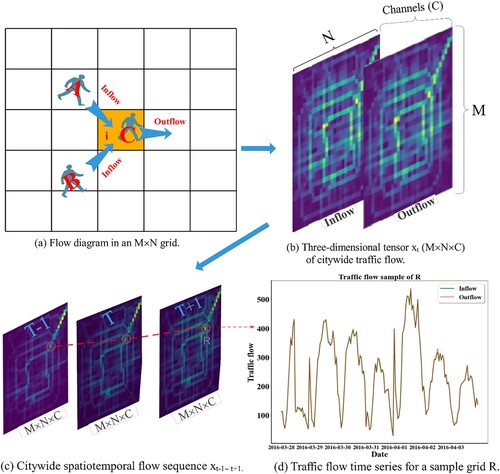
The trajectory and intensity of human movement exhibit not only spatial characteristics such as spatial heterogeneity and dependence but also temporal characteristics such as closeness (hours), periodicity (days) and trend (weeks). In terms of the spatial characteristics, Figure 1(a) shows an example of the traffic flow in Beijing, China. The spatial grids $\mathrm{i}$, A, and B are inflow objects, and C is an outflow object. By gridding urban traffic flows in a similar manner, inflows and outflows can be easily recorded and predicted. The recorded inflow and outflow grids are combined into a three-dimensional tensor $X_t^{M\times N\times C}$, as shown in Figure 1(b). In this case, M×N denotes the number of grids over the city, and C denotes the number of channels, i.e. the inflow and outflow, respectively; hence, C = 2. Notably, traffic flows exhibit distinct spatial characteristics: Stronger traffic flows correspond to more hotspot grids, although certain cold spot traffic flow grids also exist. However, this traffic flow grid corresponds to only a particular moment t. The spatial flows that occur in the period between t-1 to t+1 form urban spatiotemporal flow tensors $X_{t-1\sim t+1}^{M\times N\times C}$, as shown in Figure 1(c). A sample grid R with prominent traffic flows is selected to record the time series of traffic flow, as shown in Figure 1(d). The peaks and troughs of the time series exhibit a clear cyclical pattern. Thus, urban traffic flow is a spatiotemporal process in which spatial and temporal features are fused. It is difficult to realize accurate end-to-end traffic flow prediction by extracting only spatial or temporal features of urban traffic flows for modeling. Thus, spatiotemporal fusion modeling is a crucial yet challenging aspect.

Figure 1. Spatiotemporal volumes of citywide traffic flows in Beijing.

DL, as a group of data-driven modeling techniques, excels in spatiotemporal modeling due to its powerful feature extraction and nonlinear fitting capabilities compared to those of traditional model-driven statistical methods. Convolutional techniques are representative techniques in DL for modeling the spatial feature extraction of images. A CNN unit is a neural network that connects to the local patches in the feature maps of the previous layer through a set of weights known as convolution kernels (Lecun, Bengio, and Hinton 2015). By combining multilayer convolutional networks, traffic flow feature extraction at different time nodes can be performed. A well-known multilayer CNN structure of the U-Net model, which stacks the traffic flow tensors of all time points, has been developed to realize end-to-end forecasting (Konyakhin, Lukashina, and Shpilman 2021); however, this model cannot consider the temporal characteristics of closeness (hours), periodicity (days) and trend. Another multilayer CNN structure model, DeepST, uses historical observations from hourly ($X^{M\times N\times H}$), daily ($X^{M\times N\times D}$), and weekly ($X^{M\times N\times W}$) patterns to effectively and simultaneously capture spatial and temporal characteristics (Zhang et al. 2016). To avoid the problem of deep network degradation of multilayer convolution, ST-ResNet, a spatiotemporal residual model based on DeepST incorporating a residual network, was proposed by Zhang et al. (2018). Notably, ST-ResNet empirically divides the input data into hourly and daily segments, which may lead to improper division. An ST-ResNet-TB model attenuates this division error by introducing a time buffer. All these modeling approaches simply stack convolutional layers and thus cannot effectively capture the temporal dependence of traffic flows. An LSTM is a typical technique for modeling the temporal relationship of time series data. However, the ST-ResNet-TB and U-Net models do not adopt LSTM to more effectively capture temporal properties. Many researchers have attempted to integrate CNN and LSTM techniques to enhance the spatiotemporal modeling and forecasting of urban traffic flows. The Hybrid-LR model represents the first implementation of a combination of convolutional networks with LSTM to capture spatiotemporal features in prediction. In the Hybrid-LR model, the inputs are separately fed into a ResNet model and an LSTM model, and the outputs are merged using a parametric matrix-based method (Yuankai and Tan 2016). However, the temporal and spatial feature extraction of the Hybrid-LR model is implemented separately. A ConvLSTM framework can effectively fuse a convolution network with LSTM to simultaneously capture spatiotemporal features (Shi et al. 2015). Notably, a ConvLSTM module can capture only a single temporal feature in terms of the closeness (hours), periodicity (days) and trend (weeks). A hybrid integrated DL model (HIDLST) captures the temporal dependencies of hourly, daily, and weekly patterns through three ConvLSTM modules. Thus, relative to the aforementioned models, HIDLST-based spatiotemporal forecasting systems can realize end-to-end forecasting with an enhanced forecasting accuracy (Ren et al. 2020).

In HIDLST frameworks, although feature extraction is realized using three ConvLSTMs, each ConvLSTM model assigns the same importance to each grid and each channel in the M×N×C tensor. As shown in Figure 1, the traffic flow grids exhibit distinct spatial features, with the traffic flow on the grid in which the main roads are located being significantly more prominent than that on the right-of-way. Thus, among the $M\times N$ grids, more attention should be assigned to intersection grids with high traffic flow. Similarly, the feature maps of different inflow/outflow channels (C) must be assigned different attention levels. Attention mechanisms have been extensively examined in the existing studies. Drawing on human attention mechanisms, attention clarifies the focus area to the model and enhances the representation of interest. Attention mechanisms are introduced in the HIDLST model to enhance the feature extraction, focus more on important grids and feature channels, and suppress unnecessary grids and feature channels.

3. Methodology

As mentioned previously, urban traffic flows can be gridded into three-dimensional spatiotemporal tensor sequences ($X_{t-i\sim t+i}^{M\times N\times C}$), as shown in Figure 1. Urban traffic flow prediction is therefore equivalent to a multidimensional spatiotemporal tensor prediction problem, which can be mathematically expressed as $X_t^{M\times N\times C}$  = F (X_ST, E). X_ST denotes the set of historical spatiotemporal flow tensors, $X_t^{M\times N\times C}$ denotes the prediction target at time t, and E represents other influencing factors. The difficulty of prediction lies in accurately and simultaneously modeling the spatiotemporal relationships. To address this problem, in this study, an attention-based hybrid spatiotemporal model, named the attention-based HIDLST (Figure 2), is proposed.

Figure 2. Framework of the attention-based HIDLST model.

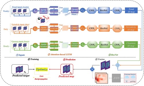
The attention-based HIDLST model consists of six modules: an input module (Inputs), a temporal feature extraction module (Attention-based ConvLSTM), a spatial feature extraction module (ResNet), a fusion module (Fusion), a prediction module (Prediction), and a training module (Training). The input module performs the dynamic partitioning of feature subsets by introducing adjustable temporal parameters. The novel attention-based ConvLSTM incorporates spatial attention and channel attention in the traditional ConvLSTM model to efficiently extract the temporal dependencies and spatiotemporal heterogeneity of the traffic flow in each subset. The traditional ResNet module extracts the spatial dependencies through convolution operations. Finally, the fusion module with a parameter matrix realizes the fusion of each feature subset. In this manner, the attention-based HIDLST model can efficiently extract and model spatiotemporal relationships through these six modules. The following sections describe the main modules of attention-based HIDLST.

3.1. Input module with a time buffer

The urban traffic flow at time $t$ is gridded to form a three-dimensional tensor ($X_t^{M\times N\times C}$), and the tensors at different time points in history are concatenated to form a spatiotemporal tensor sequence, such as an hourly sequence tensor $X_H^{h\times M\times N\times C}$. As shown in Figure 1(d), gridded urban traffic flow has temporal characteristics, such as closeness, periodicity and trend (Zhang et al. 2018).

In terms of the closeness pattern in gridded flows, the traffic flow in an urban area is closely related to the flows in recent time intervals, both near and far. For instance, the traffic flow at 9:00 am is closely related to those at 8:00 am, 7:00 am and even 6:00 am, as traffic congestion from 6:00–8:00 am during the morning peak hours affects the traffic flow at 9:00 am. To capture the hourly patterns of traffic flow, we select $t$ to represent the target time. $X_H$ denotes the hourly input dataset, which includes three-dimensional tensors, as mentioned previously. The dataset can be expressed as in Equation (1(1) $\begin{array}{c}{X}_H^{h\times M\times N\times 2}=\left(\begin{array}{c}{X}_{t-h},\dots ,X_{t-i},\\ \dots ,X_{t-2},X_{t-1}\end{array}\right),\left\{iϵZ|1\le i\le h\right\}\end{array}$(1) ): (1) $\begin{array}{c}{X}_H^{h\times M\times N\times 2}=\left(\begin{array}{c}{X}_{t-h},\dots ,X_{t-i},\\ \dots ,X_{t-2},X_{t-1}\end{array}\right),\left\{iϵZ|1\le i\le h\right\}\end{array}$(1) where $h$ refers to the length of each time interval corresponding to the hourly pattern, and $M\times N$ is the grid size of the city traffic flow. In Figure 2, the closeness inputs present an instance in which $h=3.$

In terms of the periodic pattern in traffic flow, traffic conditions may be similar during the morning peak hours on consecutive weekdays, and this pattern may repeat every 24 h. For example, the traffic flow at 9:00 am on one morning may be similar to that on the previous morning or two mornings prior at approximately 9:00 am. $X_D$ denotes the input daily dataset, which includes three-dimensional tensors, as mentioned previously. To capture a wider range of historical data, we use the time window method with a window size of $b$. $X_D$ is defined in Equation (2(2) $\begin{array}{c}{X}_D^{d\times M\times N\times 2}=\left(\begin{array}{c}{X}_{t-j\ast m-b},\dots ,X_{t-j\ast m-1},X_{t-j\ast m},\\ X_{t-j\ast m+1},\dots ,X_{t-j\ast m+b}\end{array}\right),\left\{jϵZ|1\le j\le d\right\}\end{array}$(2) ): (2) $\begin{array}{c}{X}_D^{d\times M\times N\times 2}=\left(\begin{array}{c}{X}_{t-j\ast m-b},\dots ,X_{t-j\ast m-1},X_{t-j\ast m},\\ X_{t-j\ast m+1},\dots ,X_{t-j\ast m+b}\end{array}\right),\left\{jϵZ|1\le j\le d\right\}\end{array}$(2) where $d$ denotes the number of time intervals corresponding to the daily pattern, $m$ is the number of time intervals in one day, and b is the size of the time buffer. In Figure 2, the periodic inputs present an instance in which $d=1$ and b = 1.

In terms of the trend pattern in traffic flows, the weekly pattern cannot be ignored when a long trend exists. $X_W$ denotes the input weekly dataset, which includes three-dimensional tensors, as mentioned previously. Moreover, the dataset contains a time buffer, as shown in Equation (3(3) $\begin{array}{c}{X}_W^{w\times M\times N\times 2}=\left(\begin{array}{c}{X}_{t-k\ast 7\ast m-b},\dots ,X_{t-k\ast 7\ast m-1},X_{t-k\ast 7\ast m}\\ ,X_{t-k\ast 7\ast m+1},\dots ,X_{t-k\ast 7\ast m+b}\end{array}\right)\end{array}$(3) ): (3) $\begin{array}{c}{X}_W^{w\times M\times N\times 2}=\left(\begin{array}{c}{X}_{t-k\ast 7\ast m-b},\dots ,X_{t-k\ast 7\ast m-1},X_{t-k\ast 7\ast m}\\ ,X_{t-k\ast 7\ast m+1},\dots ,X_{t-k\ast 7\ast m+b}\end{array}\right)\end{array}$(3) where $w$ denotes the number of time intervals corresponding to the weekly pattern, and b refers to the size of the time buffer. In Figure 2, the trend inputs present an instance in which $w=1$ and b = 1.

The introduction of adjustable time intervals and time buffer parameters enables the input module to dynamically partition the closeness, periodicity, and trend datasets.

3.2. Attention-based ConvLSTM module for capturing the temporal dependency

The attention-based ConvLSTM module includes three parts: spatial attention, LSTM, and channel attention. The core function is to capture the temporal dependencies of traffic flows. As described previously, the $X_H$,$X_D$, and $X_w$ datasets are divided to extract the hourly, daily, and weekly patterns of traffic flows, respectively. We consider the hourly pattern as an example to illustrate the procedure (Figure 3).

Figure 3. Structure of the attention-based ConvLSTM module.

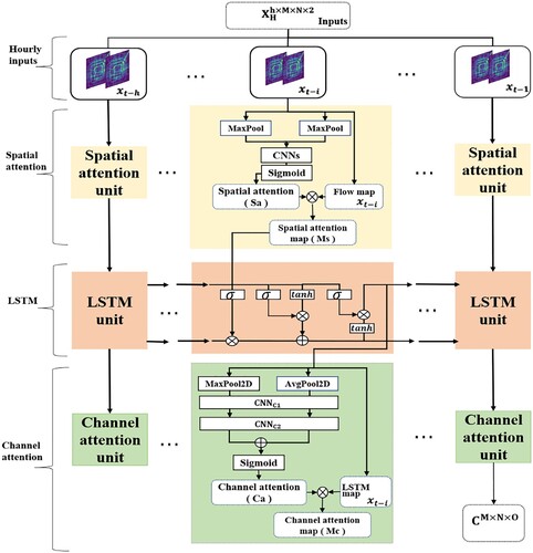
An hourly attention-based ConvLSTM module receives the tensor $X_H^{h\times M\times N\times 2}$, which includes the traffic flow volumes for h hours approaching the target time t. At time $t-i$, the feature tensor is expressed as $X_{t-i}^{M\times N\times 2}$. As shown in Figure 3, a pooling operation is implemented to extract the spatially highlighted information, to which more attention (weight) must be assigned in the spatial attention module (Woo et al. 2018). The application of pooling operations along the channel axis has been shown to be effective in highlighting informative regions (Zagoruyko and Komodakis 2017). Thus, using average pooling and max pooling operations, we obtain two spatial context descriptors: $P_{t-i\left(s\mathrm{\_}avg\right)}^{M\times N}$ and $P_{t-i\left(s\mathrm{\_}max\right)}^{M\times N}$, which denote the average-pooled features and max-pooled features, respectively. Using the concatenated feature descriptor, the average-pooled features ($P_{t-i\left(s\mathrm{\_}avg\right)}^{M\times N}$) and max-pooled features ($P_{t-i\left(s\mathrm{\_}max\right)}^{M\times N}$) are concatenated into a spatial feature tensor ($P_{t-i\left(s\right)}^{M\times N\times 2}$). Subsequently, using a CNN with a sigmoid activation function, the spatial attention (weight) ($S_{t-i\left(s\right)}^{M\times N\times 2}$) is generated. Spatial attention is weighted onto the traffic flow feature map by multiplying the weight matrix and feature map. Finally, a spatial attention feature map ($M_{t-i\left(s\right)}^{M\times N\times 2}$) at time $t-i$ is obtained. Equation (4(4) $\begin{array}{rl}{M}_{t-i\left(s\right)}^{M\times N\times 2}& =\sigma \left(f_{CN{N}_s}\right(\left[AvgPool\left(X_{t-i}^{M\times N\times 2}\right);MaxPool\left(X_{t-i}^{M\times N\times 2}\right)\right]\left)\right)\\ & =\sigma \left(f_{CN{N}_s}\right(\left[P_{t-i\left(s\mathrm{\_}avg\right)}^{M\times N};P_{t-i\left(s\mathrm{\_}max\right)}^{M\times N}\right]\left)\right)\\ & =\sigma \left(f_{CN{N}_s}\right(P_{t-i\left(s\right)}^{M\times N\times 2}\left)\right)\\ & =S_{t-i\left(s\right)}^{M\times N\times 2}\otimes X_{t-i}^{M\times N\times 2}\end{array}$(4) ) describes the procedure of spatial attention generation: (4) $\begin{array}{rl}{M}_{t-i\left(s\right)}^{M\times N\times 2}& =\sigma \left(f_{CN{N}_s}\right(\left[AvgPool\left(X_{t-i}^{M\times N\times 2}\right);MaxPool\left(X_{t-i}^{M\times N\times 2}\right)\right]\left)\right)\\ & =\sigma \left(f_{CN{N}_s}\right(\left[P_{t-i\left(s\mathrm{\_}avg\right)}^{M\times N};P_{t-i\left(s\mathrm{\_}max\right)}^{M\times N}\right]\left)\right)\\ & =\sigma \left(f_{CN{N}_s}\right(P_{t-i\left(s\right)}^{M\times N\times 2}\left)\right)\\ & =S_{t-i\left(s\right)}^{M\times N\times 2}\otimes X_{t-i}^{M\times N\times 2}\end{array}$(4) where $AvgPool$ and $MaxPool$ denote the average pooling and max pooling operations, respectively.

The traffic flow tensors of h hours are sequentially passed through the spatial attention unit to generate the final spatial attention-weighted tensors. To capture the temporal dependence of the traffic flow at hour h, the LSTM is implemented on the tensors with spatial attention weighting. The LSTM captures the dynamic temporal dependencies underlying the time series through a unique structure involving an input gate, a forgetting gate, and an output gate in each LSTM cell. In the LSTM module, the output of the last cell (t-1) is a candidate traffic flow feature map $\left(M_{st}^{M\times N\times O}\right)$ with temporal characteristics, where $M\times N$ denotes the size of the traffic grid, and O denotes the number of hidden neurons in the LSTM layer, which also indicates the number of extracted feature channels. This candidate feature tensor includes spatial attention-weighted temporal-dependent information. Equation (5(5) $\begin{array}{c}{M}_{st}^{M\times N\times O}=f_{lstm}\left(M_{t-h\left(s\right)}^{M\times N\times 2},\dots ,M_{t-i\left(s\right)}^{M\times N\times 2},\dots ,M_{t-1\left(s\right)}^{M\times N\times 2}\right)\end{array}$(5) ) describes the procedure of LSTM: (5) $\begin{array}{c}{M}_{st}^{M\times N\times O}=f_{lstm}\left(M_{t-h\left(s\right)}^{M\times N\times 2},\dots ,M_{t-i\left(s\right)}^{M\times N\times 2},\dots ,M_{t-1\left(s\right)}^{M\times N\times 2}\right)\end{array}$(5) where $M_{t-i\left(s\right)}^{M\times N\times 2}$ denotes the spatial attention-weighted feature map at time $t-i$, and $M_{st}^{M\times N\times O}$ denotes the candidate feature tensor containing the spatial attention-weighted and temporal-dependent information.

In the HIDLST model, a convolutional layer directly extracts the candidate feature maps with multiple channels $\left(M_{st}^{M\times N\times O}\right)$ as the corresponding two-channel feature maps of the input tensor. However, the acquired feature tensor has O channels, and not all features in each channel are equally important for the traffic flow prediction. Therefore, based on the attention mechanism, we introduce channel attention to assign weights to the channel features or different attention levels to different channel features (Woo et al. 2018). Similarly, the maximum and average pooling operations for channel attention help extract the average-pooled and max-pooled features in the channel dimension, as shown in Figure 3. In contrast to the spatial pooling operations, each feature channel consists of a two-dimensional feature map $\left(M_{st}^{M\times N}\right)$. Only the two-dimensional (2D) pooling operation enables the extraction of max-pooled features and average-pooled features. Therefore, two feature tensors, $P_{stc\mathrm{\_}max}^{1\times 1\times O}$ and $P_{stc\mathrm{\_}avg}^{1\times 1\times O},$, are generated through two-dimensional maximum pooling (MaxPool 2D) and two-dimensional average pooling (AvgPool 2D) operations, respectively. To obtain the final channel attention levels (weights), a two-layer convolutional network is used. The first layer is a convolutional layer (CNNc₁) with a convolutional kernel size of 1×1, hidden neuron units sized O/${\mathrm{r}}^{\mathrm{\prime }}$ and a rectified linear unit (ReLU) activation function (Maas, Hannun, and Ng 2013). A reduction ratio (${\mathrm{r}}^{\mathrm{\prime }}$) is introduced to decrease the parameter overhead. The subsequent layer is a convolutional layer (CNNc₂) with a convolutional kernel size of 1×1, hidden neuron unit sized O and sigmoid activation function. The channel attention ($C_{stc}^{1\times 1\times O}$) is generated by convoluting the two pooled features $(P_{stc\mathrm{\_}max}^{1\times 1\times O},$ $P_{stc\mathrm{\_}avg}^{1\times 1\times O})$ through these two layers and adding them. Finally, a candidate feature tensor $\left(M_{stc}^{M\times N\times O}\right)$ with the spatiotemporal attention weight and temporal-dependent features is generated by multiplying the channel attention ($C_{stc}^{1\times 1\times O}$) and feature tensor ($M_{st}^{M\times N\times O}$) output from the LSTM network. Equation (6(6) $\begin{array}{rl}{M}_{stc}^{M\times N\times O}& =\sigma \left(f_{CN{N}_{c2}}\left(f_{CN{N}_{c1}}\right(\mathrm{M}\mathrm{a}\mathrm{x}\mathrm{P}\mathrm{o}\mathrm{o}\mathrm{l}2\mathrm{D}\left(M_{st}^{M\times N\times O}\right),\mathrm{A}\mathrm{v}\mathrm{g}\mathrm{P}\mathrm{o}\mathrm{o}\mathrm{l}2\mathrm{D}\left(M_{st}^{M\times N\times O}\right))\right))\\ & =\sigma \left(f_{CN{N}_{c2}}\left(f_{CN{N}_{c1}}\right(P_{stc\mathrm{\_}max}^{1\times 1\times O},P_{stc\mathrm{\_}avg}^{1\times 1\times O})\right))\\ & =\sigma (C_{stc\mathrm{\_}max}^{1\times 1\times O}+C_{stc\mathrm{\_}avg}^{1\times 1\times O})\\ & =\sigma \left(C_{stc}^{1\times 1\times O}\right)\\ & =C_{stc}^{1\times 1\times O}\otimes M_{st}^{M\times N\times O}\end{array}$(6) ) describes the procedure of channel attention: (6) $\begin{array}{rl}{M}_{stc}^{M\times N\times O}& =\sigma \left(f_{CN{N}_{c2}}\left(f_{CN{N}_{c1}}\right(\mathrm{M}\mathrm{a}\mathrm{x}\mathrm{P}\mathrm{o}\mathrm{o}\mathrm{l}2\mathrm{D}\left(M_{st}^{M\times N\times O}\right),\mathrm{A}\mathrm{v}\mathrm{g}\mathrm{P}\mathrm{o}\mathrm{o}\mathrm{l}2\mathrm{D}\left(M_{st}^{M\times N\times O}\right))\right))\\ & =\sigma \left(f_{CN{N}_{c2}}\left(f_{CN{N}_{c1}}\right(P_{stc\mathrm{\_}max}^{1\times 1\times O},P_{stc\mathrm{\_}avg}^{1\times 1\times O})\right))\\ & =\sigma (C_{stc\mathrm{\_}max}^{1\times 1\times O}+C_{stc\mathrm{\_}avg}^{1\times 1\times O})\\ & =\sigma \left(C_{stc}^{1\times 1\times O}\right)\\ & =C_{stc}^{1\times 1\times O}\otimes M_{st}^{M\times N\times O}\end{array}$(6) where $\mathrm{M}\mathrm{a}\mathrm{x}\mathrm{P}\mathrm{o}\mathrm{o}\mathrm{l}2\mathrm{D}$ and $\mathrm{A}\mathrm{v}\mathrm{g}\mathrm{P}\mathrm{o}\mathrm{o}\mathrm{l}2\mathrm{D}$ denote two-dimensional average pooling and max pooling operations, respectively, and $C_{stc}^{1\times 1\times O}$ refers to the channel attention (weight).

3.3. ResNet module for capturing the spatiotemporal dependency

The ResNet module captures the spatiotemporal dependency based on the output ($M_{stc}^{M\times N\times O}$) of the attention-based ConvLSTM. In this module, ResNet is adopted to avoid the problem of deep network degradation, as shown in Figure 4.

Figure 4. Structure of the ResNet module.

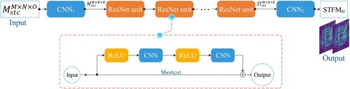
First, $M_{stc}^{M\times N\times O}$ serves as the input of this module. A convolutional layer (CNN₁) transforms the input into a feature tensor with the same dimensionality as that of the output of ResNet. Each ResNet unit includes a stack of two ‘ReLU + CNN’ layers with a shortcut connection linking the input and output of the second CNN layer (He et al. 2016; Zhang et al. 2018). Finally, a convolutional layer (CNN₂) converts the ResNet output into a two-channel hourly spatiotemporal feature map (hourly ST-map: STFM_H). Equation (7(7) $\begin{array}{rl}\mathrm{S}\mathrm{T}\mathrm{F}{\mathrm{M}}_H& =f_{CN{N}_2}\left(f_{Resnet}\left(f_{CN{N}_1}\right(M_{stc}^{M\times N\times O})\right))\\ & =f_{CN{N}_2}\left(f_{CN{N}_{Resnet}}\right(M_{stc}^{M\times N\times K}\left)\right)\\ & =f_{CN{N}_2}\left(S{T}_{stc}^{M\times N\times K}\right)\end{array}$(7) ) describes the procedure of the ResNet module. (7) $\begin{array}{rl}\mathrm{S}\mathrm{T}\mathrm{F}{\mathrm{M}}_H& =f_{CN{N}_2}\left(f_{Resnet}\left(f_{CN{N}_1}\right(M_{stc}^{M\times N\times O})\right))\\ & =f_{CN{N}_2}\left(f_{CN{N}_{Resnet}}\right(M_{stc}^{M\times N\times K}\left)\right)\\ & =f_{CN{N}_2}\left(S{T}_{stc}^{M\times N\times K}\right)\end{array}$(7) where $\mathrm{S}\mathrm{T}\mathrm{F}{\mathrm{M}}_H$ denotes the spatiotemporal feature map with $M\times N\times 2$ dimensions, and $f_{CN{N}_1},f_{CN{N}_2},$ and $f_{Resnet}$ refer to the convolution and ResNet operations.

3.4. Fusion and prediction modules

Three modules pertaining to closeness, periodicity, and trend extract hourly $\left(\mathrm{S}\mathrm{T}\mathrm{F}{\mathrm{M}}_H\right)$, daily $\left(\mathrm{S}\mathrm{T}\mathrm{F}{\mathrm{M}}_D\right)$, and weekly $STF{M}_W$ spatiotemporal feature maps, respectively. However, the fusion module is implemented to not only fuse these three feature maps but also consider the fusion of external factors. External factors, such as the weather, temperature, and holidays, considerably influence urban traffic flows (Tanner 1952). Crowd flows during holidays may be significantly different from flows during normal days. To consider the influence of external factors during the prediction process, an external factor feature map ($E^{M\times N\times 2}$) is obtained through two layers of ANNs. In addition, a study based on the use of the ST-ResNet model to predict the same type of city traffic flow showed that although different regions are affected by the closeness, periodicity, and trend, the degrees of influence may be different (Zhang et al. 2018). Considering these aspects, we adopt a fusion strategy similar to those used in the existing studies. The parametric matrix-based method, which can be expressed as in Equation (8(8) $\begin{array}{c}STF{M}_F^{M\times N\times 2}=\mathrm{t}\mathrm{a}\mathrm{n}\mathrm{h}(\mathrm{S}\mathrm{T}\mathrm{F}{\mathrm{M}}_H\times W_H+\mathrm{S}\mathrm{T}\mathrm{F}{\mathrm{M}}_D\times W_D+\mathrm{S}\mathrm{T}\mathrm{F}{\mathrm{M}}_w\times W_w+E^{M\times N\times 2}\times W_E)\end{array}$(8) ), is used to fuse the traffic flow feature maps with an external factor feature map (Zhang et al. 2018). The final traffic flow prediction map is $X_t^{M\times N\times 2}$, which is represented as $STF{M}_F^{M\times N\times 2}$. (8) $\begin{array}{c}STF{M}_F^{M\times N\times 2}=\mathrm{t}\mathrm{a}\mathrm{n}\mathrm{h}(\mathrm{S}\mathrm{T}\mathrm{F}{\mathrm{M}}_H\times W_H+\mathrm{S}\mathrm{T}\mathrm{F}{\mathrm{M}}_D\times W_D+\mathrm{S}\mathrm{T}\mathrm{F}{\mathrm{M}}_w\times W_w+E^{M\times N\times 2}\times W_E)\end{array}$(8) where $STF{M}_F^{M\times N\times 2}$ denotes the final traffic flow prediction map; $W_H$, $W_D$, and $W_w$ are three parameter matrices with the same shape as that of the traffic flow feature map; $E^{M\times N\times 2}$ refers to the external factor map; and $W_E$ is a parameter matrix with the same shape as that of the external factor map.

3.5. Training module

In the training module, the traditional training methods of gradient descent and a backpropagation algorithm for depth models are adopted. In addition, several advanced training strategies are used. First, in the model training process, a loss function is used to evaluate the differences between the predicted and true values, and the mean-squared error (MSE) is used as an evaluation metric. The root-mean-square error (RMSE) (i.e. the square root of the MSE), defined as in Equation (9(9) $\begin{array}{c}RMSE=\sqrt{MSE}=\sqrt{{\displaystyle \frac{1}{Z}\sum _i{\left(x_i-{\hat{x}}_i\right)}^2}}\end{array}$(9) ), is adopted for model validation. Second, to evaluate the generalizability of the proposed model, the dataset can be divided into a training set, an evaluation set, and a test set for training, evaluation, and testing, respectively. Third, the model parameters are typically adjusted during the training process by using an optimization algorithm to achieve the lowest possible loss. In this study, however, we use an adaptive learning rate method (Adam) to avoid excessive adjustments of the learning rate parameter (Kingma and Ba 2015). Fourth, to prevent overfitting during model training, an early stopping measure is adopted (Prechelt 1998). When the RMSE does not decrease after seven loops, the training process is terminated. Finally, in addition to the optimization algorithm with an adaptive learning rate, we adopt a learning rate decay strategy, i.e. polynomial decay, to accelerate the convergence of the algorithm. When the RMSE does not decrease significantly after five loops, the learning rate is decreased. (9) $\begin{array}{c}RMSE=\sqrt{MSE}=\sqrt{{\displaystyle \frac{1}{Z}\sum _i{\left(x_i-{\hat{x}}_i\right)}^2}}\end{array}$(9) where $x$ and $\hat{x}$ represent the actual and predicted values, respectively; and z is the total number of observed values.

4. Case study

4.1. Study area and data

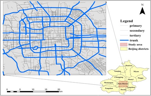
Beijing is the capital of China and a first-tier city with a large population, an active economy, and well-developed transportation systems. By 2019, the resident population had reached 21.53 million (Beijing Statistical Bureau 2019). For a large number of travelers, cars are an important mode of urban transportation. In 2013, taxis completed an average of 1.9 million trips per day in Beijing, accounting for 6.6% of the total trips (Beijing Statistical Bureau 2013). The high density of people traveling has led to severe traffic congestion in Beijing, especially in Beijing's Ring Roads motorway. The study area is a 32$k{m}^2$ square region located in one of the main districts in Beijing (Figure 5). We obtain the traffic flow data of this region from 1 November 2015–9 April 2016 through the GPS positioning system used by taxis and generate the spatiotemporal flow (including inflow and outflow) with a cell size of 1$k{m}^2$ in a 30 min interval.

Figure 5. Study area.

4.2. Experimental environment and data preparation

The programming environment can be described as follows. The programming language is Python 3.7. Keras and TensorFlow, open-source libraries for DL, are adopted (Abadi 2016; Chollet 2018). An NVIDIA GeForce GTX 2080 with 8 GB of GPU memory is used as the main computing platform.

Data preprocessing mainly involves the partitioning and normalization of the traffic flow dataset. Data for the period between 3 April 2016 and 9 April 2016 are used as the test set, and the remaining data are divided into a training set and validation set in a ratio of 9:1. Since the traffic flow and its influencing factors (i.e. the external factors) are measured in different units, to enhance the convergence speed of the model, we normalize all the data such that the data values lie between −1 and 1.

4.3. Fine-tuning of model parameters

The fine-tuning and optimization of model parameters are of significance for depth networks to achieve optimal performance. In the attention-based HIDLST model, the parameters of the input patterns and hyperparameters of the model must be tuned and optimized. To identify the optimal values of the parameters for the input patterns, we fix the hyperparameters of the model as follows: the sizes of the hidden neuron units in the LSTM and ResNet models are set as 32 and 64, respectively; the convolution kernel sizes in the LSTM and ResNet models are set as 3$\times$3; and the depths of the LSTM and ResNet are set as two and five layers, respectively.

4.3.1. Parameters of the input patterns

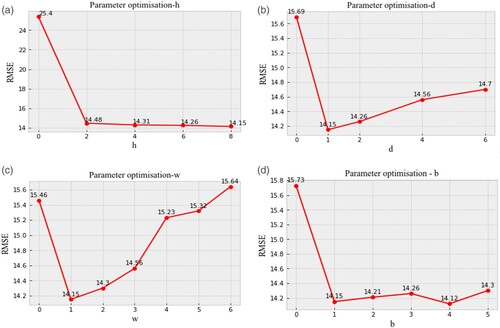
As mentioned previously, the parameters h, d, and w denote the input lengths of the hourly, daily, and weekly data patterns, respectively. The parameter b is a time buffer. To determine the optimal value of h, we fix the parameter values as follows: d = 1, w = 1, b = 1 and $h\in \left\{0,1,2,3,4,5,6,7,8\right\}$. As shown in Figure 6(a), when h = 8, the minimum RMSE is 14.15. If the model omits the hourly pattern (h = 0), the RMSE is maximized. This finding shows that the hourly pattern is crucial for prediction. Subsequently, we fix the parameter values as h = 8, w = 1, b = 1 and $d\in \left\{0,1,2,3,4,5,6\right\}$, as shown in Figure 6(b). The minimum RMSE is 14.15 when d is 1. Similarly, the RMSE is minimized when w is 1, as shown in Figure 6(c). The RMSEs of the three patterns first decrease and later increase. Therefore, the RMSE is minimized when h = 8, d = 1, and w = 1. This finding suggests that the daily and weekly effects on prediction are not as prominent as those of the hourly pattern. Finally, to determine the optimal time buffer b, we fix the parameter values as h = 8, d = 1, w = 1 and $b\in \left\{0,1,2,3,4,5\right\}$. As shown in Figure 6(d), when b = 4, the minimum RMSE is 14.12, indicating that the traffic at four adjacent time points is closely related to the traffic at the target time point. The optimal parameters for the input patterns are as follows: h = 8, d = 1, w = 1, and b = 4, with the minimum RMSE being 14.12.

Figure 6. Optimization results for the input patterns. a. Hourly parameter h. b. Daily parameter d. c. Weekly parameter w. d. Time buffer b.

4.3.2. Hidden neuron size

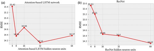
It is necessary to optimize the sizes of the hidden neurons in the attention-based ConvLSTM and ResNet modules of the proposed attention-based HIDLST model. Using the optimal parameter values for the input patterns and a fixed size for the convolution kernel, we first identify the optimal hidden neuron size ($F{S}_{LSTM}$) of the attention-based ConvLSTM. The hidden neuron size ($F{S}_{ResNet}=64$) of ResNet is fixed, and $F{S}_{LSTM}$ is assigned values of 4, 8, 16, 32, and 64. When $F{S}_{LSTM}$ is 32, the minimum RMSE is 14.12, as shown in Figure 7(a). Subsequently, the hidden neuron size ($F{S}_{LSTM}=32$) of the LSTM is fixed, and $F{S}_{ResNet}$ is assigned values of 4, 8, 16, 32, and 64. When $F{S}_{ResNet}$ is 64, the minimum RMSE is 14.12, as shown in Figure 7(b). Thus, the optimal hidden neuron sizes for the attention-based ConvLSTM and ResNet modules are 32 and 64, respectively, corresponding to the minimum RMSE.

Figure 7. Optimization results for the hidden neuron size parameter. a.$F{S}_{\mathrm{L}\mathrm{S}\mathrm{T}\mathrm{M}}$. b.$F{S}_{\mathrm{R}\mathrm{e}\mathrm{s}\mathrm{N}\mathrm{e}\mathrm{t}}$.

4.3.3. Convolution kernel size

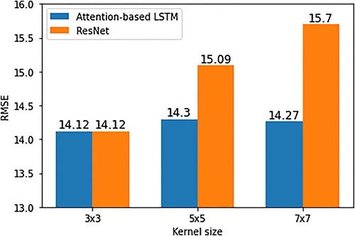
The convolution kernel size determines the perceptual domain of the local region. To identify the optimal convolutional kernel size, we fix the convolutional kernel size of ResNet as 3×3 and convolutional kernel sizes of the CNN layer in the attention-based ConvLSTM modules as 3×3, 5×5, and 7×7. When the convolution kernel size of the attention-based ConvLSTM is 3×3, the minimum RMSE is 14.12, as shown in Figure 8. Although larger convolutional kernels perceive larger ranges, multilayer small kernels capture more complex nonlinear features (Simonyan and Zisserman 2015). Thus, we fix the optimal convolutional kernel size of the attention-based ConvLSTM network as 3×3 and convolutional kernel sizes of ResNet as 3×3, 5×5, and 7×7. When the convolution kernel size of the two modules is 3×3, the obtained minimum RMSE is 14.12, as shown in Figure 8.

Figure 8. Optimization results for the convolution kernel size parameter.

4.3.4. Network depth

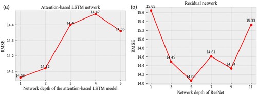
The depth of the neural network is a key factor for optimizing the model fitting performance. Although deeper network layers correspond to a stronger model fitting ability, the model may suffer from more significant network degradation. This problem can be addressed by using residual networks. To this end, the depth of ResNet is first fixed as five layers, and the depth of the attention-based ConvLSTM ranges from one to five. When the depth of the attention-based ConvLSTM is 1, the minimum RMSE is 14.06, as shown in Figure 9(a). For the optimal depth of the attention-based ConvLSTM model, the minimum RMSE is 14.06 when the depth of ResNet is five, as shown in Figure 9(b). Finally, the optimal depth for the attention-based HIDLST method corresponds to the configuration in which the LSTM has one layer and ResNet has five layers. Compared to the optimal two-layer LSTM in HIDLST, the optimal LSTM in the attention-based HIDLST method requires only one layer, indicating that by introducing the attention mechanism, the prediction accuracy can be enhanced using a network with fewer layers.

Figure 9. Optimization results for the network depth parameter. a. Depth of the attention-based ConvLSTM model. b. Depth of ResNet.

4.4. Model comparison

To validate the performance of the proposed attention-based HIDLST model, we compare the prediction accuracy of the attention-based HIDLST with that of the abovementioned six models under the same experimental conditions. As shown in Table 1, the LSTM model, which does not consider spatial characteristics, corresponds to the largest prediction error. This finding indicates that significant spatial heterogeneity exists in urban traffic flows, which must be considered to realize a reasonable prediction. Although the ConvLSTM method increases the accuracy of LSTM by simultaneously extracting spatial and temporal features, it does not distinguish between hourly, daily, and weekly traffic flow patterns, which leads to high computational costs and long-term resource consumption. The ST-ResNet model distinguishes different traffic flow patterns, while the ST-ResNet-TB model decreases the pattern segmentation errors by introducing time buffers into the ST-ResNet model. However, the temporal dependency is ignored in both the ST-ResNet and ST-ResNet-TB models. The Hybrid-LR model incorporates the LSTM for extracting temporal dependencies and ResNet for extracting spatial attributes. However, the processes of providing inputs for the two modules of the Hybrid-LR model are implemented separately; consequently, the performance of the Hybrid-LR model is not as high as that of ST-ResNet and ST-ResNet-TB. The HIDLST model uses three input modules to simultaneously address the abovementioned issues of extracting spatiotemporal features and discovering different patterns that are difficult to simultaneously consider. However, the calculation time of the HIDLST model is high, second only to that of the ConvLSTM model. The proposed attention-based HIDLST model introduces an attention mechanism to decrease the computational consumption and increase the prediction accuracy under the framework of the HIDLST model. The prediction accuracy and computational consumption are optimized for the 6 models. Compared to the HIDLST model, the proposed attention-based HIDLST model achieves a 3.7% reduction in RMSE and 60.09% reduction in the runtime. The results of the comparison experiment demonstrate that by introducing the attention mechanism into the HIDLST, the proposed model requires the least number of training iterations and least time, and the prediction accuracy is significantly enhanced. In addition, when channel attention and spatial attention are separately applied to the HIDLST model, the increase in the prediction efficiency of the HIDLST model corresponding to the introduction of the spatial attention module is more notable than that of the channel attention module.

Table 1. Results of the comparison experiment.

Model	RMSE	Iterations	Time (s)
LSTM*	16.59	118	5005
ConvLSTM*	15.76	201	10940
ST-ResNet*	15.81	101	1798
ST-ResNet-TB*	15.32	87	1602
Hybrid-LR*	15.37	101	2651
HIDLST*	14.60	120	2903
HIDLST with spatial attention	14.26	79	1580
HIDLST with channel attention	14.40	94	1874
Attention-based HIDLST	14.06 (3.7%$\downarrow$)	63 (47.5%$\downarrow$)	1134 (60.9$\text{\%}\downarrow$)

Note: *Results of certain models are extracted from an existing study (Ren et al. 2020).

5. Discussion

5.1. Performance with the attention mechanism

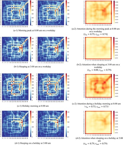
To analyse the patterns of traffic flow intensity and attention (weight), we consider the data associated with the morning peak hour (8:00 am) and midnight (3:00 am) on a weekday (5 April 2016) and a nonworking day (9 April 2016), respectively, to explore the correlations. As shown in Figure 10, the traffic flow exhibits hotspots during sleeping and nonsleeping hours on weekdays and nonworking days. The traffic hotspots are consistent with the attention map. This result suggests that more attention (weight) must be assigned to traffic hotspots; in other words, a more prominent traffic flow must be assigned higher attention. Furthermore, we examine the relationship between the traffic intensity and attention by calculating Pearson correlation coefficients (Benesty et al. 2009). All correlation coefficients (r) are greater than 0.70 at different times, indicating a strong positive correlation between the attention and traffic. The model exhibits a high performance when attention mechanisms are incorporated, regardless of the time or life mode examined.

Figure 10. Attention maps at different times.

5.2. Spatiotemporal distribution of forecasting errors

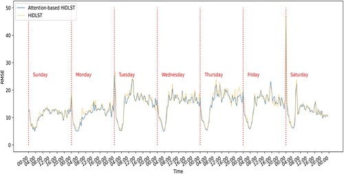
To explore the spatial and temporal distribution of the forecasting errors, the analysis was separately performed in temporal and spatial dimensions. In the temporal dimension, the RMSEs of 2048 (32×32×2) grids in the time dimension are computed. As shown in Figure 11, the introduction of an attention mechanism decreases the overall error compared to that associated with the HIDLST model. In addition, the errors exhibit daily periodicity: the errors are smaller at night than those in the day on both working and nonworking days. The sparse traffic flow at midnight exhibits smaller prediction errors than those of the high-intensity traffic flow in the morning and evening peak hours. This finding indicates that the predictions are highly erroneous when high-intensity and variable traffic flows occur. Nevertheless, the overall prediction errors of the proposed model for the morning and evening peak traffic flows are smaller than those of the HIDLST model. These results show that the prediction errors in regions with low or variable traffic flows can be decreased by introducing an attention mechanism. In addition, Saturday, 9 April, is the first day of the weekend, and the prediction error is the largest at the start of 9 April, indicating that more people engage in trips and other activities at the start of the weekend than at other times. Consequently, a large variation is introduced in the traffic flow model, and the variable traffic pattern renders accurate traffic prediction challenging.

Figure 11. Prediction errors in the time dimension.

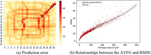
In the spatial dimension, we explore the spatial distribution of the obtained forecasting errors by calculating the average value of the traffic flow (AVFG) and RMSE for each grid cell. As shown in Figure 12(a), a high spatial consistency exists between the prediction error and traffic flow intensity. Higher prediction errors often appear at traffic hotspots. This finding suggests that predictions associated with locations with high and variable traffic volumes are more challenging to obtain than those for other locations. Figure 12(b) shows the trend lines fitted through a cubic function. The results indicate that the prediction error increases as the traffic flow intensity increases. Moreover, the black line lies lower than the red line, demonstrating that the prediction error of the attention-based model is lower than that of the model without attention in hot areas with high traffic. This result provides valuable evidence that the introduction of an attention mechanism can increase the prediction accuracy in traffic hotspots.

Figure 12. Prediction errors in the spatial dimension.

5.3. Generalizability of the proposed model

The proposed attention-based HIDLST model outperforms other models in urban traffic flow prediction. However, the model must be generalizable for predictions in other contexts. As mentioned previously, the proposed model can be applied in situations in which spatiotemporal characteristics must be simultaneously modeled and the modeling can be transformed into a similar multidimensional spatiotemporal tensor modeling problem, such as population flow patterns, bicycle flow patterns, work check-in and check-out patterns, and taxi pick-up patterns. To this end, we conduct a prediction study of taxi passenger pick-up patterns based on Shanghai data to verify the prediction ability of the attention-based HIDLST model.

Taxis represent a valuable transportation mode for urban residents. The accurate prediction of taxi loading patterns can not only facilitate taxi acquisition in peak hours but also allow taxi drivers to accurately predict the passenger demand at different locations and times. The difficulty in forecasting urban traffic flow can be alleviated by gridding the flows. Each grid includes two characteristic channels: inflow and outflow. Similarly, the passenger carrying patterns of taxis are gridded; each grid cell includes two feature channels corresponding to the number of pick-ups and number of drop-offs. The predicted spatiotemporal tensors are similar in the Shanghai and Beijing cases. However, Shanghai lacks distinct road features such as Beijing's Ring Roads, and the traffic hotspots radiate mainly from the center, as shown in Figure 13(b).

Figure 13. Validation experiments.

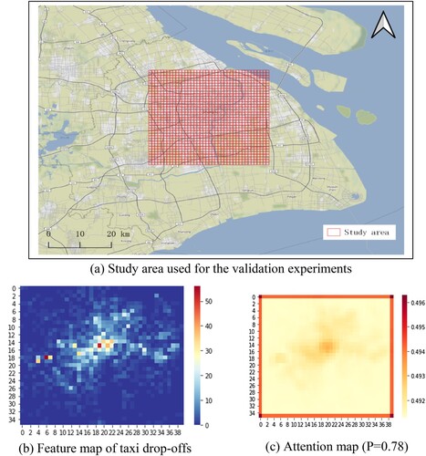
The validation area is in the main city of Shanghai with an area of 36×40 km² (Figure 13(a)). The validation data are taxi GPS data and order data for April 2015. A dataset with 1440×36×40×2 dimensions is obtained through the same data processing approach. When the attention mechanism is incorporated in the prediction process, the Shanghai taxi-carrying pattern predictions are excellent, even in the absence of distinct traffic flow features such as those associated with Beijing's Ring Roads. Compared to that of the HIDLST model (13.98), the RMSE of the attention-based model is 13.61, corresponding to a decrease of 2.65%. As shown in Figure 13(c), the attention map and passenger-carrying feature map exhibit a high consistency in hotspots, with a correlation coefficient of as high as 0.78. The validation experiment demonstrates the high generalizability of the proposed attention-based HIDLST model.

6. Conclusions and future work

This paper proposes an attention-based hybrid spatiotemporal residual model, which is an end-to-end dynamic model, by incorporating an attention mechanism into the HIDLST. By employing spatial and channel attention modules, the problems that lead to large prediction errors in hot spot areas, cold spot areas, and variable areas owing to the assignment of equal attention levels (weights) can be solved. The proposed model decreases the computational cost and significantly increases the accuracy of prediction. The prediction performance of the model is evaluated considering a Beijing traffic flow case and Shanghai taxi validation case. In the case of Beijing traffic flow forecasting, the prediction accuracy and efficiency of the proposed model are significantly higher than those of the six traditional DL models including the HIDLST. For high-traffic hotspots, the attention and traffic flow exhibit a high consistency. Moreover, the issue of occurrence of large traffic prediction errors at hotspots in morning or evening peak hours can be adequately addressed by the proposed model. The prediction accuracy of the model for cold spots and regions with varied traffic in midnight hours is enhanced. In addition, to evaluate the model performance in different forecasting contexts, a case study is performed to predict the taxi ridership in the main city of Shanghai. The results show that the proposed model outperforms the models that do not consider the attention mechanism.

In summary, the proposed attention-based HIDLST model can automatically and accurately capture the spatiotemporal features of urban traffic flows and achieve accurate predictions with low overhead. The prediction results can not only facilitate the travel of citizens but also provide accurate planning references for city managers. Notably, although the model introduces a time buffer to adjust the input hourly, daily, and weekly patterns, the attention-based HIDLST model must be enhanced in terms of the optimization of the input parameters and hyperparameters, for instance, by using an automated approach for parameter optimization. Moreover, even though the practicability of the model is verified through a case study of taxi-carrying pattern prediction, the applicability of the attention mechanism to other spatiotemporal prediction scenarios, such as crowd flows, bike flows, and migration flows, could be examined. Future work will be aimed at establishing an attention-based spatiotemporal model that is more widely applicable and easier to use.

Data availability statement

The authors confirm that the Beijing’s traffic flow data supporting the findings of this study are available within the website (https://github.com/p0llx/DeepST-ResNet/tree/master/data/TaxiBJ). Additional data related to this study may be requested from the corresponding authors.

Disclosure statement

No potential conflict of interest was reported by the author(s).

Additional information

Funding

This work was supported by National Key R&D Program of China: [grant number 2017YFB0503605].

References

- Abadi, M. 2016. “TensorFlow: Learning Functions at Scale.” ACM SIGPLAN Notices 51 (9): 1. doi:10.1145/3022670.2976746.
- Abadi, A., T. Rajabioun, and P. A. Ioannou. 2014. “Traffic Flow Prediction for Road Transportation Networks with Limited Traffic Data.” IEEE Transactions on Intelligent Transportation Systems 16 (2): 653–662. doi:10.1109/tits.2014.2337238.
- Bao, Y., T. Xiong, and Z. Hu. 2014. “Multi-Step-Ahead Time Series Prediction Using Multiple-Output Support Vector Regression.” Neurocomputing 129: 482–493. doi:10.1016/j.neucom.2013.09.010.
- Beijing Statistical Bureau. 2013. Beijing Statistical Yearbook of Transportation. Beijing, China: China Statistics Publishing House.
- Beijing Statistical Bureau. 2019. Beijing Statistical Yearbook. Beijing, China: China Statistics Publishing House.
- Benesty, J., J. Chen, Y. Huang, and I. Cohen. 2009. “Pearson Correlation Coefficient.” In Noise Reduction in Speech Processing. Springer Topics in Signal Processing, 1–4. Berlin, Heidelberg: Springer.
- Bengio, Y., and O. Delalleau. 2011. “On the Expressive Power of Deep Architectures.” In Lecture Notes in Computer Science (Including Subseries Lecture Notes in Artificial Intelligence and Lecture Notes in Bioinformatics, edited by J. Kivinen, C. U. Szepesvári, and E. T. Zeugmann, 18–36. Berlin, Heidelberg: Springer.
- Bui, K. H. N., J. Cho, and H. Yi. 2021. “Spatial-Temporal Graph Neural Network for Traffic Forecasting: An Overview and Open Research Issues.” Applied Intelligence, 1–12. doi:10.1007/s10489-021-02587-w.
- Chen, C., J. Hu, Q. Meng, and Y. Zhang. 2011. “Short-Time Traffic Flow Prediction with ARIMA-GARCH Model.” In 2011 IEEE Intelligent Vehicles Symposium (IV), 607–612. Baden-Baden, Germany: IEEE.
- Chollet, F. 2018. “Introduction to Keras.” March 9th.
- Çolak, S., A. Lima, and M. C. González. 2016. “Understanding Congested Travel in Urban Areas.” Nature Communications 7 (1): 10793. doi:10.1038/ncomms10793.
- Fu, R., Z. Zhang, and L. Li. 2017. “Using LSTM and GRU Neural Network Methods for Traffic Flow Prediction.” 2016 31st Youth Academic Annual Conference of Chinese Association of Automation (YAC), 324-328.Wuhan, China: IEEE.
- He, K., X. Zhang, S. Ren, and J. Sun. 2016. “Identity Mappings in Deep Residual Networks.” In Lecture Notes in Computer Science (Including Subseries Lecture Notes in Artificial Intelligence and Lecture Notes in Bioinformatics, edited by B. Leibe, J. Matas, N. Sebe, and M. Welling, 630–645. Cham: Springer.
- Hochreiter, S., and J. Schmidhuber. 1997. “Long Short-Term Memory.” Neural Computation 9 (8): 1735–1780. doi:10.1162/neco.1997.9.8.1735.
- Huang, J., L. Zheng, J. Qin, D. Xia, L. Chen, and D. Sun. 2019. “Short-Term Travel Time Prediction on Urban Road Networks Using Massive ERI Data.” In 2019 IEEE SmartWorld, Ubiquitous Intelligence & Computing, Advanced & Trusted Computing, Scalable Computing & Communications, Cloud & Big Data Computing, Internet of People and Smart City Innovation (SmartWorld/SCALCOM/UIC/ATC/CBD), 582–588. Leicester, UK: IEEE.
- Kim, S. H., J. Shi, A. Alfarrarjeh, D. Xu, Y. Tan, and C. Shahabi. 2013. “Real-Time Traffic Video Analysis Using Intel Viewmont Coprocessor.” In Lecture Notes in Computer Science (Including Subseries Lecture Notes in Artificial Intelligence and Lecture Notes in Bioinformatics), edited by A. Madaan, S. Kikuchi, and S. Bhalla, 150–160. Berlin, Heidelberg: Springer.
- Kingma, D. P., and L. J. Ba. 2015. “Adam: A Method for Stochastic Optimization.” In 3rd International Conference on Learning Representations, ICLR 2015 - Conference Track Proceedings, 13. Ithaca, NY.
- Konyakhin, V., N. Lukashina, and A. Shpilman. 2021. “Solving Traffic4Cast Competition with U-Net and Temporal Domain Adaptation.” arXiv preprint arXiv:2111.03421.
- Lecun, Y., Y. Bengio, and G. Hinton. 2015. “Deep Learning.” Nature 521 (7553): 436–444. doi:10.1038/nature14539.
- Liu, H. X., X. He, and W. Recker. 2007. “Estimation of the Time-Dependency of Values of Travel Time and its Reliability from Loop Detector Data.” Transportation Research Part B: Methodological 41 (4): 448–461. doi:10.1016/j.trb.2006.07.002.
- Ma, Z., H. N. Koutsopoulos, L. Ferreira, and M. Mesbah. 2017. “Estimation of Trip Travel Time Distribution Using a Generalized Markov Chain Approach.” Transportation Research Part C: Emerging Technologies 74: 1–21. doi:10.1016/j.trc.2016.11.008.
- Ma, X., Z. Tao, Y. Wang, H. Yu, and Y. Wang. 2015. “Long Short-Term Memory Neural Network for Traffic Speed Prediction Using Remote Microwave Sensor Data.” Transportation Research Part C: Emerging Technologies 54: 187–197. doi:10.1016/j.trc.2015.03.014.
- Maas, A. L., A. Y. Hannun, and A. Y. Ng. 2013. “Rectifier Nonlinearities Improve Neural Network Acoustic Models.” ICML Workshop on Deep Learning for Audio, Speech and Language Processing 30 (1): 3.
- Moussa, G. S., and M. Owais. 2020. “Pre-Trained Deep Learning for Hot-Mix Asphalt Dynamic Modulus Prediction with Laboratory Effort Reduction.” Construction and Building Materials 265: 120239. doi:10.1016/j.conbuildmat.2020.120239.
- Moussa, G. S., and M. Owais. 2021. “Modeling Hot-Mix Asphalt Dynamic Modulus Using Deep Residual Neural Networks: Parametric and Sensitivity Analysis Study.” Construction and Building Materials 294: 123589. doi:10.1016/j.conbuildmat.2021.123589.
- Owais, M., G. S. Moussa, and K. F. Hussain. 2020. “Robust Deep Learning Architecture for Traffic Flow Estimation from a Subset of Link Sensors.” Journal of Transportation Engineering, Part A: Systems 146 (1): 04019055.
- Parida, M., K. Kumar, and V. K. Katiyar. 2013. “Short Term Traffic Flow Prediction for a Non Urban Highway Using Artificial Neural Network.” Procedia - Social and Behavioral Sciences 104: 755–764. doi:10.1016/j.sbspro.2013.11.170.
- Prechelt, L. 1998. “Early Stopping - But When?” In Neural Networks: Tricks of the Trade, edited by G. B. Orr, and K.-R. Müller, 55–69. Berlin, Heidelberg: Springer.
- Ren, Y., H. Chen, Y. Han, T. Cheng, Y. Zhang, and G. Chen. 2020. “A Hybrid Integrated Deep Learning Model for the Prediction of Citywide Spatio-Temporal Flow Volumes.” International Journal of Geographical Information Science 34 (4): 802–823. doi:10.1080/13658816.2019.1652303.
- Robinson, S., and J. W. Polak. 2005. “Modeling Urban Link Travel Time with Inductive Loop Detector Data by Using the k-NN Method.” Transportation Research Record 1935 (1): 47–56. doi:10.1177/0361198105193500106.
- Shi, X., Z. Chen, H. Wang, D. Y. Yeung, W. K. Wong, and W. C. Woo. 2015. “Convolutional LSTM Network: A Machine Learning Approach for Precipitation Nowcasting.” In Advances in Neural Information Processing Systems 28: 802–810.
- Simonyan, K., and A. Zisserman. 2015. “Very Deep Convolutional Networks for Large-Scale Image Recognition.” arXiv preprint arXiv:1409.1556.
- Smith, B. L., B. M. Williams, and R. K. Oswald. 2002. “Comparison of Parametric and Nonparametric Models for Traffic Flow Forecasting.” Transportation Research Part C: Emerging Technologies 10 (4): 303–321. doi:10.1016/S0968-090X(02)00009-8.
- Song, C., Z. Qu, N. Blumm, and A.-L. Barabási. 2010. “Limits of Predictability in Human Mobility.” Science 327 (5968): 1018. doi:10.1126/science.1177170.
- Tang, J., F. Liu, Y. Zou, W. Zhang, and Y. Wang. 2017. “An Improved Fuzzy Neural Network for Traffic Speed Prediction Considering Periodic Characteristic.” IEEE Transactions on Intelligent Transportation Systems 18 (9): 2340–2350. doi:10.1109/TITS.2016.2643005.
- Tanner, J. C. 1952. “Effect of Weather on Traffic Flow.” Nature 169 (4290): 107. doi:10.1038/169107a0.
- Uherek, E., T. Halenka, J. Borken-Kleefeld, Y. Balkanski, T. Berntsen, C. Borrego, M. Gauss, et al. 2010. “Transport Impacts on Atmosphere and Climate: Land Transport.” Atmospheric Environment 44 (37): 4772–4816. doi:10.1016/j.atmosenv.2010.01.002.
- Williams, B. M., and L. A. Hoel. 2003. “Modeling and Forecasting Vehicular Traffic Flow as a Seasonal ARIMA Process: Theoretical Basis and Empirical Results.” Journal of Transportation Engineering 129 (6): 664–672. doi:10.1061/(ASCE)0733-947X(2003)129:6(664).
- Woo, S., J. Park, J.-Y. Lee, and I. S. Kweon. 2018. “CBAM: Convolutional Block Attention Module.” In Lecture Notes in Computer Science (Including Subseries Lecture Notes in Artificial Intelligence and Lecture Notes in Bioinformatics, edited by V. Ferrari, M. Hebert, C. Sminchisescu, and Y. Weiss, 3–19. Cham: Springer.
- Xie, Y., Y. Zhang, and Z. Ye. 2007. “Short-Term Traffic Volume Forecasting Using Kalman Filter with Discrete Wavelet Decomposition.” Computer-Aided Civil and Infrastructure Engineering 22 (5): 326–334. doi:10.1111/j.1467-8667.2007.00489.x.
- Xiong, X., K. Ozbay, L. Jin, and C. Feng. 2020. “Dynamic Origin–Destination Matrix Prediction with Line Graph Neural Networks and Kalman Filter.” Transportation Research Record 2674 (8): 491–503. doi:10.1177/0361198120919399.
- Yuankai, W., and H. Tan. 2016. “Short-term traffic flow forecasting with spatial-temporal correlation in a hybrid deep learning framework.” arXiv preprint arXiv:1612.01022.
- Zagoruyko, S., and N. Komodakis. 2017. “Paying more Attention to Attention: Improving the Performance of Convolutional Neural Networks via Attention Transfer.” arXiv preprint arXiv:1612.03928.
- Zhan, X., S. Hasan, S. V. Ukkusuri, and C. Kamga. 2013. “Urban Link Travel Time Estimation Using Large-Scale Taxi Data with Partial Information.” Transportation Research Part C: Emerging Technologies 33: 37–49. doi:10.1016/j.trc.2013.04.001.
- Zhan, X., Y. Zheng, X. Yi, and S. V. Ukkusuri. 2017. “Citywide Traffic Volume Estimation Using Trajectory Data.” IEEE Transactions on Knowledge and Data Engineering 29 (2): 272–285. doi:10.1109/TKDE.2016.2621104.
- Zhang, L., T. Hu, Y. Min, G. Wu, J. Zhang, P. Feng, P. Gong, and J. Ye. 2017. “A Taxi Order Dispatch Model Based on Combinatorial Optimization.” Proceedings of the ACM SIGKDD International Conference on Knowledge Discovery and Data Mining, 2151-2159.
- Zhang, J., Y. Zheng, D. Qi, R. Li, and X. Yi. 2016. “DNN-Based Prediction Model for Spatio-Temporal Data.” GIS: Proceedings of the ACM International Symposium on Advances in Geographic Information Systems 1–4.
- Zhang, J., Y. Zheng, D. Qi, R. Li, X. Yi, and T. Li. 2018. “Predicting Citywide Crowd Flows Using Deep Spatio-Temporal Residual Networks.” Artificial Intelligence 259: 147–166. doi:10.1016/j.artint.2018.03.002.
- Zheng, C., X. Fan, C. Wen, L. Chen, C. Wang, and J. Li. 2020. “DeepSTD: Mining Spatio-Temporal Disturbances of Multiple Context Factors for Citywide Traffic Flow Prediction.” IEEE Transactions on Intelligent Transportation Systems 21 (9): 3744–3755. doi:10.1109/TITS.2019.2932785.
- Zheng, M., T. Li, R. Zhu, J. Chen, Z. Ma, M. Tang, Z. Cui, and Z. Wang. 2019. “Traffic Accident’s Severity Prediction: A Deep-Learning Approach-Based CNN Network.” IEEE Access 7: 39897–39910. doi:10.1109/ACCESS.2019.2903319.