Winter wheat leaf area index inversion by the genetic algorithms neural network model based on SAR data

ABSTRACT

The leaf area index (LAI) is an important agroecological physiological parameter affecting vegetation growth. To apply the genetic algorithms neural network model (GANNM) to the remote sensing inversion of winter wheat LAI throughout the growth cycle and based on GaoFen-3 Synthetic aperture radar (GF-3 SAR) images and GaoFen-1 Wide Field of View (GF-1 WFV) images, the Xiangfu District in the east of Kaifeng City, Henan Province, was selected as the testing region. Winter wheat LAI data from five growth stages were combined, and optical and microwave polarization decomposition vegetation index models were used. The backscattering coefficient was extracted by modified water cloud model (MWCM), and the LAI was obtained by MWCM inversion as input factors to construct GANNM to invert LAI. The root mean square error (RMSE) and determination coefficient (R²) were used as evaluation indicators of the model. The fitting accuracy of winter wheat LAI in five growth stages by GANNM inversion was better than that of the BP neural network model; the R² was higher than 0.8, and RMSE was lower than 0.3, indicating that the model could accurately invert the growth status of winter wheat in five growth stages .

KEYWORDS:

• Leaf area index (LAI)
• GF-3
• BP neural network model (BPNNM)
• genetic algorithms neural network model
• winter wheat

1. Introduction

The leaf area index (LAI) is an important vegetation structure parameter in the biogeochemical cycle (Katsuhama et al. 2018; Le Maire et al. 2012; Prévot, Champion, and Guyot 1993). In this paper, LAI was defined as half of the sum of the total leaf area per unit surface area (Ren et al. 2018). LAI is an important index for estimating vegetation coverage, monitoring and forecasting crop growth, biomass, yield, etc. Therefore, the rapid and accurate inversion of LAI is of great research significance for agricultural monitoring and biogeochemical cycles.

Remote sensing technology is an effective method for regional or global crop LAI monitoring due to its advantages of a large coverage area and efficiency. Based on optical remote sensing images, the main approaches of LAI remote sensing inversion consist of an optical vegetation index model and a physical model, but the inversion accuracy of the two models is subject to whether the optical remote sensing images are covered by clouds or not, which leads to poor reliability and universality.

Due to its capacity of all-weather and all-time, synthetic aperture radar (SAR) can penetrate clouds and a dense vegetation canopy and has great application potential in vegetation parameter inversion and monitoring. Based on SAR remote sensing images, the main means of LAI remote sensing inversion are the empirical model and cloud-water model. The empirical model uses the backscattering coefficients of Horizontal transmit and horizontal received (HH), Horizontal transmit and vertical received (HV), and Vertical transmit and vertical received (VV) polarization modes to establish a correlation with the measured LAI (Inoue et al. 2002; Xu et al. 2016; Wali, Tasumi, and Moriyama 2020). However, the above models lacked a physical basis, and different empirical models need to be established in different environments of each region, making their generalization poor.

The water cloud model (WCM) is a semi-empirical parameter inversion model first proposed by Attema and Ulaby in 1978 (Attema and Ulaby 1978). Due to its simplicity and practicability, WCM has been widely applied in numerous subsequent inversion studies on soil moisture and vegetation growth parameters (Kweon and Yisok 2015; Ulaby et al. 1984; Xu 1996; Yadav, Prasad, and Bala 2021; Yang et al. 2016). However, the above models required too many parameters, and artificial measurement error or the lack of some input parameters in the process led to large errors and uncertainties in the physical model. Furthermore, the secondary scattering component was not considered in WCM, and secondary scattering between the vegetation canopy and the underlying surface was ignored. However, secondary scattering contributes to the overall backscattering, especially in the early stage of the vegetation growth cycle. Based on SAR data, the use of SAR is advantageous because microwaves are sensitive to the structure and dielectric constant of ground objects, and shortwave multipolarization SAR is widely used in the parameter inversion fields of LAI. However, based on SAR data, empirical modeling methods are simple and easy to operate but lack theoretical support and depend largely on modeling data and vegetation types and characteristics. The physical model was established by simulating the physical processes of scattering, emission, and absorption of microwaves in the vegetation canopy or underlying surface. Although the vegetation LAI inversion process by physical modeling is complex, it has strong theoretical support and can be used to analyze the interaction mechanism between SAR backscattering microwaves and the vegetation canopy.

In summary, the inversion of the LAI model based on optical images is vulnerable to cloud coverage, leading to low inversion accuracy, and the inversion of LAI in the whole growth stage of winter wheat also lacks verification. Based on GF-3 SAR images and GF-1 WFV images, this paper considered optical and microwave polarization decomposition vegetation index models, backscattering coefficients extracted from modified water cloud model (MWCM), and LAI obtained from MWCM inversion as input factors, and a genetic algorithms neural network model (GANNM) inversion method for winter wheat LAI in five growth stages was proposed. This method combined optical and radar remote sensing and made full use of their respective advantages to invert surface parameters, which can improve inversion accuracy.

2. Materials and methods

2.1. Materials

2.1.1. Study area

For this study, the Xiangfu District (34°30′–34°56′ N, 114°07′–114°43′ E) in the eastern part of Kaifeng City, Henan Province, which belongs to the Yellow River alluvial plain, was selected. It has an average altitude of 62.5–89.3 m, an average annual temperature of 14°C, an average annual precipitation of 628 mm, and an average frost-free period of 214 days. A temperate continental monsoon climate provides sufficient sunshine, suitable temperatures, and abundant precipitation, which is conducive to crop growth. The location of the study region and the distribution of sampling points are shown in Figure 1.

Figure 1. Location of the study region and distribution of sampling points. (a) Location of Xiangfu District in Henan Province; (b) Location of leaf area index sampling points; (c) Leaf area index, Global Positioning System, and soil moisture was measured at each sampling site.

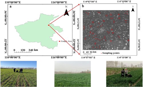
2.1.2. Satellite data collection and processing

In this paper, GF-3 SAR and GF-1 WFV data within the study area were selected and downloaded from the China Centre for Resources Satellite Data and Application (CCRSDA). Among them, the GF-3 SAR data band was the C band, incidence angles ranged from 20–41°, the transit times were March 14, March 19, April 29, May 28, and June 04, 2020. The operating frequency was 5.4 GHz, and spatial resolution was 8 m. The images were processed by full polarization introduction, radiometric calibration, amplitude enhancement, and speckle filtering, and four scattering components were extracted by Yamaguchi polarimetric decomposition of the processed data. Using TanDEM-X elevation model data (DEM), the GF-3 SAR data were calibrated to sigma nought via the calibration factors and the sine of the local incidence angle derived from the TanDEM-X DEM. To reduce speckle noise, Speckle filtering used a Boxcar 5 × 5 kernel filter. Sigma nought radiometric calibration was performed according to the absolute calibration coefficients downloaded from CCRSDA (http://www.cresda.com/CN/).

The transit times of GF-1 WFV images were March 14, March 19, April 29, May 28, and June 05, 2020. The image level was 1A, and the spatial resolution was 16 m. The width was 800 km, and the revisit period was 4 days. Atmospheric correction and ortho-rectification were carried out on the images. FLAASH atmospheric correction was adopted to obtain the true reflectivity of the surface. Ortho-rectification was conducted using RPC and DEM elevation data to make the images more accurate and clearer. Based on GF-1 WFV images, DEM used 90-m resolution data in this study, downloaded from the SRTM 90 m DEM Digital Elevation Database (https://srtm.csi.cgiar.org/).

2.1.3. Field data observation

This experiment aimed to prevent changes in weather conditions from affecting the accuracy of the measured LAI. The experiment analyzed the LAI inversion of winter wheat in five growth stages; the selected acquisition dates were March 9, March 24, April 25, May 29, and June 04, 2020, which were almost synchronous with the satellite transit time. The daily acquisition time was 07:30–09:30 am Fifty winter wheat quadrats with a size of 16 m × 16 m were selected, and three spots with the same growth status were chosen. All quadrats had to be at least 30 m from trees, buildings, and roads. When sampling, sunlight was shielded, and LAI-2000 was used for measurement; specifically, a 180° covering cap was used to ensure that there was no error in measurement. In addition, the distance between the measured ground and the instrument was adjusted to 5 cm, according to the standard, to ensure that there was no error between the winter wheat canopy and the viewing angle range of the instrument. To avoid errors in measuring LAI, the LAI of each sample site was measured four times, and the average value was taken as the end value. Using Stevens Hydra probes, volumetric soil moisture ($M_S$) was measured at each sampling site. For each sampling site, three replicates of dielectric permittivity were measured at a depth of 6 cm. Calibration of the probe measurements was achieved by developing site specific calibration equations based on gravimetric sampling, resulting in an average root mean square error (RMSE) of 0.037 m³/m³. Furthermore, the longitude and latitude of each winter wheat sampling point was recorded in real time using a U.S. Global Positioning System (GPS) locator. Figure 1 illustrates the measurements of winter wheat LAI, soil moisture, and sampling point location.

2.2. Methods

The model was built by studying the correlation between winter wheat LAI and GF-3 full polarimetric data and GF-1 WFV data. For GF-1 WFV and GF-3 SAR data, the correlation between optical and microwave polarization decomposition vegetation index models and LAI was analyzed, while for GF-3 SAR data, the correlation between the backscattering coefficient obtained by MWCM and the measured LAI was analyzed. Finally, the backscattering coefficient obtained by MWCM, LAI obtained by MWCM inversion, and the optical and microwave polarization decomposition vegetation index model were used as input factors of GANNM. The stability of the BP neural network and the fitness ratio of the genetic algorithm, real number crossover, and mutations were adopted to enhance the training and optimization search ability and obtain better LAI inversion accuracy, as shown in Figure 2.

Figure 2. Flowchart of leaf area index inversion by GANNM.

2.2.1. Selection of the optical and microwave polarization decomposition vegetation index model

To eliminate the influence of insufficient reflectivity caused by complex terrain, the Xiangfu District, Kaifeng, Henan Province was selected as the testing region, where the backscattering mainly came from surface, vegetation canopy, and leaf secondary scattering. Therefore, Yamaguchi polarimetric decomposition (Niu et al. 2021; Xu et al. 2011) was introduced in this paper, which can decompose fully polarimetric SAR into scattering power components of four scattering mechanisms to construct a polarization decomposition vegetation index according to four scattering proportions. The total covariance matrix $T_4$ was as follows: (1) $T_4=F_s{C}_v+F_d{C}_d+F_v{C}_s+F_h{C}_h$(1) where, $C_v$, $C_d$, $C_s$, and $C_h$ represent volume, secondary, surface, and spiral scattering, respectively, and $F_s$, $F_d$, $F_v$, and $F_h$, respectively, correspond to the contributions of the four scattering quantities. In this paper, the polarization decomposition index $RV{I}_{Yamaguchi}$ was defined according to $C_v$ as follows: (2) $RV{I}_{Yamaguchi}=C_v/\left(C_v+C_d+C_s+C_h\right)$(2)

When the GF-3 satellite irradiates dense vegetation, since the scattering energy incidence on the ground is small, the energy incidence on the ground and reflected to the leaves and stems of the vegetation decreases, namely $C_d$ and $C_s$ decrease, but dense vegetation will make $C_v$ and $C_h$ increase, with little influence from $C_h$. At this time, the value of RVI approaches 1. When GF-3 irradiates bare land, the volume scattering amount $C_v$ will approach 0, and the RVI will also approach 0.

When LAI is inverted by an optical image, it is easy to reach saturation when LAI is high and sensitive when LAI is low, which makes inversion inconsistent with the actual situation. Moreover, radar backscattering is very sensitive to vegetation structure and scatter number (Liao et al. 2018). Therefore, based on the advantages of GF-3 SAR images and GF-1 WFV images on LAI inversion, this paper constructed an optical and microwave polarization decomposition vegetation index model according to Yamaguchi polarimetric decomposition. Table 1 is a hybrid vegetation index model by optical and microwave polarization decomposition.

Table 1. Optical and microwave polarization decomposition vegetation index model.

Vegetation Index Type	Vegetation Index Name	Calculation Formula
Optical and microwave polarization decomposition vegetation index model	Modified normalized difference vegetation index	$\mathrm{M}\mathrm{N}\mathrm{D}\mathrm{V}\mathrm{I}=RV{I}_{Yamaguchi}\times \left[\left(P_{NIR}-P_R\right)/\left(P_{NIR}+P_R\right)\right]\times 10$	(3)
	Modified soil adjusted vegetation index	$\mathrm{M}\mathrm{S}\mathrm{A}\mathrm{V}\mathrm{I}=RV{I}_{Yamaguchi}\times \left[\left(P_{NIR}-P_R\right)\times \left(1+L\right)/\left(P_{NIR}-P_R+L\right)\right]$	(4)
	Modified ratio vegetation index	$\mathrm{M}\mathrm{R}\mathrm{V}\mathrm{I}=RV{I}_{Yamaguchi}\times \left[2.5\times P_{NIR}/P_R\right]$	(5)
	Modified enhanced vegetation index	$\mathrm{M}\mathrm{E}\mathrm{V}{\mathrm{I}}_2=RV{I}_{Yamaguchi}\times \left[2.5\times \left(P_{NIR}-P_R\right)/\left(P_{NIR}+2.4\times P_R+1\right)\right]\times 10$	(6)
	Modified soil adjusted vegetation index	$\mathrm{M}\mathrm{M}\mathrm{S}\mathrm{A}\mathrm{V}\mathrm{I}=RV{I}_{Yamaguchi}\times \left\{\left\{2\times P_{NIR}+1-\left[2\times P_{NIR}+1-{\left(2\times P_{NIR}+1\right)}^2-8\times {\left(P_{NIR}-P_R\right)}^{1/2}\right]\right\}/2\right\}$	(7)

Notes: $P_{NIR}$ and $P_R$ are the near infrared band, and red band of GF-1 WFV images, respectively. The reflectivity L is the soil-adjusted coefficient, and L = 0.5 in this paper.

2.2.2. MWCM

The WCM is an important model used to study the relationship between radar backscattering and crop parameters (Wang et al. 2021; Zhang et al. 2018), and it was calculated as follows: (8) ${\sigma }_0={\sigma }_{veg}\left(\theta \right)+{\tau }^2\left(\theta \right){\sigma }_{soil}\left(\theta \right)$(8) (9) ${\sigma }_{veg}\left(\theta \right)=A\times M\times \mathrm{c}\mathrm{o}\mathrm{s}\left(\theta \right)\times \left[1-{\tau }^2\left(\theta \right)\right],$(9) (10) ${\tau }^2\left(\theta \right)=\mathrm{e}\mathrm{x}\mathrm{p}\left[-2B\times {\displaystyle \frac{M}{cos\left(\theta \right)}}\right],$(10) where ${\sigma }_0$ is the total backscattering coefficient of the surface canopy covered by random polarimetric vegetation, ${\sigma }_{veg}\left(\theta \right)$ is the backscattering coefficient of vegetation layer, ${\sigma }_{soil}\left(\theta \right)$ is the direct surface backscattering coefficient, ${\tau }^2\left(\theta \right)$ is the double-layer attenuation factor of the radar wave penetrating crop layer, $\theta$ is the incidence angle of radar waves; M is the vegetation canopy parameter (i.e. LAI), B is a parameter that depends on vegetation type and incident electromagnetic wave frequency.

The model was built on the basis of the radiation transfer model, which only considers the volume scattering term from vegetation reflection and the backscattering of the ground after double-layer attenuation of vegetation, ignoring other forms of scattering in vegetation and soil. The radar backscattering coefficient is sensitive to the surface dielectric constant and closely related to soil moisture. According to Ulaby (Ulaby et al. 1984), ${\sigma }_{soil}\left(\theta \right)$ backscattering can be expressed as: (11) ${\sigma }_{soil}\left(\theta \right)=D\times M_S+E$(11) where D is the sensitivity of the radar to soil moisture, E is the backscattering coefficient of the soil, and $M_S$ is the soil moisture. Equations (9)–(11) were used in Equation (8), as shown in Equation (12). (12) ${\sigma }_0=A\times M\times \mathrm{c}\mathrm{o}\mathrm{s}\left(\theta \right)\times [1-{\tau }^2(\theta )\left]+\left(D\times M_S+E\right)\times \mathrm{e}\mathrm{x}\mathrm{p}\right[-2B\times M/\mathrm{c}\mathrm{o}\mathrm{s}(\theta \left)\right]$(12) Equation (12) only included SAR data information related to biophysical parameters. After incorporating the model $\left(f_{VI}\right)$ best fitted with LAI in the optical and microwave polarization decomposition vegetation index model into Equation (12), the obtained MWCM was incorporated, as shown in Equation (13). The model parameters A, E, B, and D in Equation (13) were determined by the Levenberg Marquardt non-linear least square optimization (Graham and Harris 2002). (13) ${\sigma }_0=f_{VI}\times A\times M\times \mathrm{c}\mathrm{o}\mathrm{s}\left(\theta \right)\times \left[1-{\tau }^2\left(\theta \right)\right]+\left(1-f_{VI}\right)\mathrm{e}\mathrm{x}\mathrm{p}\left[-2B\times M/\mathrm{c}\mathrm{o}\mathrm{s}\left(\theta \right)\right]\times (D\times M_S+E).$(13) MWCM is a function of some input parameters that quantify crop growth parameters and soil surface parameters. However, SAR signals are also affected by crop growth parameters, such as LAI, vegetation water content (VWC), and planting soil property ($M_S$). The backscattering coefficient in crops is expressed as follows: (14) ${\sigma }_{mod}=f\left(LAI,M_S,f_{VI}\right)$(14) The cross-polarization backscattering coefficient was mainly related to vegetation scattering. Therefore, the establishment of a look up table (LUT) under HV polarization could effectively invert the LAI from MWCM. The LUT method is by nature the direct comparison of the radiative transfer model backscattering value calculated using the GF-3 SAR image under HV against the backscattering value simulated by MWCM. It is a simple and widely used inversion method in the field of vegetation parameter retrieval from remote sensing data. LUT consisted of two main steps: LUT generation and LUT searching.

In LUT generation, 90,000 parameter combinations were first randomly generated following uniform distributions. The ranges (minimum and maximum) for each of the 5 main model parameters are summarized in Table 2.

Table 2. The range of all parameters in generating look up table

Name of parameter	Unit	Lower limit	Upper limit	Sources
$\mathrm{L}\mathrm{A}\mathrm{I}$	m^2/m^−2	0.1	7	Ground measurement
${\sigma }_{\mathrm{m}\mathrm{o}\mathrm{d}}$	dB	−12	−10	MWCM acquisition
${\sigma }_{\mathrm{o}\mathrm{b}\mathrm{s}}$	dB	−12	−10	Image acquisition
${\mathrm{M}}_{\mathrm{S}}$	%	5.9	40.1	Ground measurement
${\mathrm{f}}_{\mathrm{V}\mathrm{I}}$	No unit	0.15	0.45	Image acquisition

In LUT searching, the mean square error Z was used to represent the difference between the observed and estimated backscattering value and was expressed as: (15) $Z=\mathrm{m}\mathrm{i}\mathrm{n}\sqrt{{\displaystyle \frac{1}{N}\sum _{i=1}^n\left({\sigma }_{obs}-{\sigma }_{mod}\right)}}$(15) where ${\sigma }_{obs}$ is the backscattering value calculated using the GF-3 SAR image under HV polarization; ${\sigma }_{mod}$ is the backscattering value simulated by MWCM; and N is the number of pixel points in the image.

2.2.3. Evaluation methodology

Through accuracy evaluation, the fitting status between the model and the measured LAI of winter wheat was effectively evaluated to obtain the optimal inversion model. Two methods, namely R² (Wang et al. 2020) and RMSE (Amin et al. 2021; Gómez-Candón, Bellvert, and Royo 2021; Jafari and Keshavarz 2021), were selected to evaluate the fitting accuracy, as shown in Equations (16) and (17). (16) $R^2=1-{\displaystyle \frac{{\sum }_{i=1}^n\left(y-y_i\right)}{{\sum }_{c=1}^n\left(\mathrm{y}-y_c\right)}}$(16) (17) $\mathrm{R}\mathrm{M}\mathrm{S}\mathrm{E}=\sqrt{{\displaystyle \frac{{\sum }_{i=1}^n\left(y_e-y_d\right)}{n}}}$(17)

In Equation (16), R² is the determination coefficient, y is the measured ecological parameter value, $y_i$ is the estimated ecological parameter value, and $y_c$ is the average value of the measured ecological parameter. In Equation (17), RMSE is the root mean square error,$y_e$ is the measured LAI value; $y_d$ is the estimated LAI value; and n is the number of samples.

2.2.4. Neural network model

(1) BP neural network model

When using a back propagation neural network model (BPNNM) for LAI inversion, it is necessary to set parameters such as the number of layers, input layer, hidden layer, output layer node number, and hidden layer number. Generally, the number of neurons in the input layer and the output layer is closely related to the nature of the problem itself. To determine the number of nodes in the hidden layer and the number of hidden layers, researchers need to determine it according to the nature of the problem to be processed and their understanding and experience of BPNNM (Li et al. 2021).

This study used a 3-layer network model to construct the BP model and establish the corresponding relationship between the nine kinds of input data and LAI. When determining the network parameters, nine neurons were selected in the input layer, which corresponded to five optical and microwave polarization decomposition vegetation index models, three backscattering coefficients extracted by MWCM, and the LAI obtained by MWCM, and one neuron in the output layer was the corresponding LAI value. In contrast, the determination of the number of neurons in the hidden layer was affected by the number of neurons set in the input layer and the output layer; however, this was related to the complexity of the research problem and the characteristics of the sample data. Inappropriate selection can easily cause over- or underfitting. In this study, the final number of neurons in the hidden layer was determined through repeated experiments on empirical formulas [Equations (18)–(20)] (Wang and Qing 2021), proposed by different scholars, as shown in Table 3. (18) $H=\mathrm{l}\mathrm{o}{\mathrm{g}}_{2}I,I\in \left[0.002I,4I\right]$(18) (19) $H=\sqrt{I+O}+\alpha ,\alpha \in \left[1,10\right]$(19) (20) $H=2I+1$(20) where H is the number of neurons in the hidden layer; I is the number of neurons in the input layer, O is the number of neurons in the output layer; and $\alpha$ is a constant.

Table 3. Model accuracy index under different numbers of neurons in the hidden layer.

Equation	Number of Nodes in the Hidden Layer	R^2	RMSE
$H=\mathrm{l}\mathrm{o}{\mathrm{g}}_{2}I,I\in \left[0.002I,4I\right]$	9	0.419	0.675
	10	0.432	0.657
	11	0.536	0.569
	12	0.435	0.584
	13	0.389	0.663
$H=\sqrt{I+O}+\alpha ,\alpha \in \left[1,10\right]$	5	0.524	0.453
	6	0.513	0.456
	7	0.598	0.411
	8	0.532	0.492
	9	0.612	0.421
	10	0.787	0.253
	11	0.705	0.389
	12	0.695	0.401
	13	0.586	0.501
	14	0.553	0.536
$H=2I+1$	9	0.598	0.453
	10	0.602	0.436
	11	0.685	0.315
	12	0.632	0.376
	13	0.601	0.399

As seen in Table 3, when the number of neurons in the hidden layer was 10, the R² was 0.787, and the root mean square error (RMSE) was 0.253 after neural network training, which was better than other neural network models with different numbers of neurons in the hidden layer.

Studies on the determination of the number of hidden layers have shown that the optimal structure of BPNN can contain more than one hidden layer. Sometimes better results may be derived from the introduction of multiple hidden layers, while the number of hidden layers should not be too high; otherwise, the network will be trapped into a local extremum, leading to a poor generalization ability (Deng, Yan, and Xiao 2021). Therefore, in this study, under the premise that the number of nodes in the hidden layer was determined, the results after multiple model trainings and verifications are shown in Table 4. When the number of hidden layers was 4, the inversion effect was best.

Table 4. Model accuracy index under different numbers of hidden layers.

Number of Hidden Layers	R^2	RMSE
1	0.645	0.501
2	0.686	0.423
3	0.753	0.256
4	0.769	0.235
5	0.721	0.386
6	0.683	0.429

In summary, the parameters of the BPNNM algorithm were finally set as nine neurons in the input layer, ten neurons in the hidden layer, four hidden layers, and one neuron (LAI) in the output layer. The S-type hyperbolic tangent function was used in the hidden layer transfer function, and the output layer function was linear. The learning rate was 0.0001, and the maximum training iteration number was 1500 times.

(2) GANNM

Although BPNNM has a strong adaptive ability, the model is prone to the problems of causing prediction points to fall into local minima and a slow convergence speed (Zhao et al. 2021a). To solve this problem, this paper adopted a genetic algorithm to optimize BPNNM based on the above-mentioned BPNNM structure. The model takes advantage of the random global search optimization characteristics of the genetic algorithm to optimize and analyze the threshold and weight of the BP neural network to achieve high efficiency, fast convergence speed, and accurate prediction by quickly searching the global optimal point. The genetic algorithm optimizes the chromosome coding and fitness function of the BP neural network, expands its search range (Abadi et al. 2021; Carrabs 2021; Zhao et al. 2021b) on the basis of ensuring the high precision of network weights and thresholds, enhances the local search ability of the model, and prevents premature phenomenon (Alhijawi and Awajan 2021; Amar and Nagase 2021; Xu, Chen, and Deng 2021) by selecting a fitness ratio [Equation (21)], real number crossover [Equation (22)], and mutation [Equation (23)]. (21) $P_i=f_i/\sum _{i=1}^n{f}_i$(21) (22) $\{\begin{array}{c}{a}_x=a_x\left(1-b\right)+a_{m}b\\ a_m=a_m\left(1-b\right)+a_{i}b\end{array}$(22) (23) $X_k=X_{\mathrm{m}\mathrm{i}\mathrm{n}}+\tau \left(X_{\mathrm{m}\mathrm{a}\mathrm{x}}-X_{\mathrm{m}\mathrm{i}\mathrm{n}}\right)$(23)

In Equations (21)–(23), n is the population size; i is the probability of selection; $f_i$ is the fitness of the individual i; b and $\tau$ are random numbers; $a_x$ is the x-th chromosome at position i; $a_m$ is the m-th chromosome at position i; $X_{\mathrm{m}\mathrm{i}\mathrm{n}}$ and $X_{\mathrm{m}\mathrm{a}\mathrm{x}}$ are the minimum gene value and the maximum gene value of the initial individual, respectively; and $X_k$ is the latest gene value after mutation.

3. Results and discussion

3.1. LAI inversion by the optical and microwave polarization decomposition vegetation index model

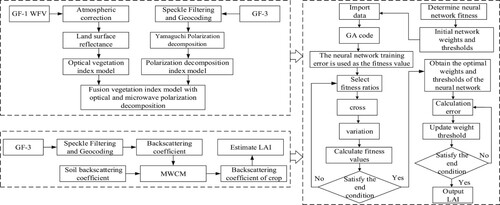
A regression model was established between the vegetation index and winter wheat LAI in the whole growth cycle by five kinds of optical and microwave polarization decomposition indices, and the accuracy was evaluated. Table 5 and Figure 3 show the evaluation of the optical and microwave polarization decomposition vegetation index model.

Figure 3. The optical and microwave polarization decomposition vegetation index models. (a–e) are from the jointing, booting, heading, filling, and maturing stages, respectively.

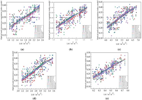
Table 5. Accuracy evaluation of the optical and microwave polarization decomposition vegetation index model.

Growth Stage	Model	R^2	RMSE	Growth Stage	Model	R^2	RMSE
Jointing	MEVI	0.632	0.3154	Booting	MEVI	0.584	0.3512
	MEVI2	0.624	0.3254		MEVI2	0.634	0.3189
	MSAVI	0.559	0.3910		MSAVI	0.623	0.3324
	MNDVI	0.723	0.2784		MNDVI	0.724	0.2746
	MMSAVI	0.589	0.3698		MMSAVI	0.574	0.3842
Heading	MEVI	0.631	0.3248	Filling	MEVI	0.624	0.3324
	MEVI2	0.658	0.2884		MEVI2	0.680	0.2995
	MSAVI	0.634	0.3125		MSAVI	0.664	0.2984
	MNDVI	0.684	0.2684		MNDVI	0.758	0.2839
	MMSAVI	0.569	0.3486		MMSAVI	0.612	0.3124
Maturing	MEVI	0.584	0.3784
	MEVI2	0.625	0.3012
	MSAVI	0.684	0.3284
	MNDVI	0.712	0.2735
	MMSAVI	0.634	0.3066

From Table 5 and Figure 3, it can be seen that in the five growth stages, the five optical and microwave polarization decomposition vegetation index models have significant inversion effects on LAI; the R² was higher than 0.5, and RMSE was lower than 0.4. Among them, the inversion accuracy of winter wheat LAI by MNDVI in the five growth stages was higher than other optical and microwave polarization decomposition vegetation index models; the R² was 0.723, 0.724, 0.684, 0.7584, and 0.7124, and RMSE was 0.3154, 0.3512, 0.2684, 0.2839, and 0.2735.

3.2. LAI inversion by MWCM

3.2.1. LAI inversion by the backscattering coefficient of MWCM

Based on GF-3 SAR images and according to Equation 14, MWCM was employed to extract the backscattering value of HH, HV, and VV polarization modes, and the correlation with measured LAI was established, as shown in Table 6 and Figure 4.

Figure 4. Correlation analysis between the backscattering coefficient model and LAI. (a–e) are from the jointing, booting, heading, filling, and maturing stages, respectively.

Table 6. Accuracy evaluation of the backscattering coefficient model.

Growth Stage	Model	R^2	RMSE	Growth Stage	Model	R^2	RMSE
Jointing	HH	0.165	0.9213	Booting	HH	0.151	0.9213
	HV	0.235	0.9010		HV	0.205	0.8922
	VV	0.155	0.9233		VV	0.113	0.9211
Heading	HH	0.159	0.9612	Filling	HH	0.166	0.9301
	HV	0.214	0.8966		HV	0.191	0.9011
	VV	0153	0.9362		VV	0.183	0.9266
Maturing	HH	0.112	0.9155
	HV	0.175	0.8863
	VV	0.153	0.9223

Because the interaction mechanism between radar and vegetation was complex and affected by surface conditions, there was no strong correlation between the three backscattering coefficients and LAI (Table 6 and Figure 4). Among them, the correlation between the HV polarization backscattering coefficient and LAI was higher than that of the HH and VV polarization backscattering coefficients because cross polarization was mainly related to vegetation volume scattering, while HH polarization better reflected the secondary and surface scattering of the surface.

3.2.2. LAI inversion by MWCM

Since the cross-polarization backscattering coefficient was mainly related to vegetation scattering, the parameters of Equation (13) in MWCM were determined by the nonlinear least squares method under HV cross polarization, as shown in Table 7. MWCM was used to invert LAI with the help of the least squares algorithm and the LUT method. Table 8 and Figure 5 show the relationship between LAI observations and predicted values of MWCM under VH polarization.

Figure 5. Correlation analysis of MWCM and LAI. (a–e) are from the jointing, booting, heading, filling, and maturing stages, respectively.

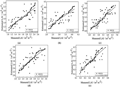
Table 7. Model parameters at HH, VV, and VH polarizations.

Polarization	Growth Stages	Model Parameters
		A	B	D	E
HV	Jointing	0.039	0.153	−11.20	19.52
	Booting	0.052	0.146	−12.12	15.33
	Heading	0.032	0.136	−9.21	16.24
	Filling	0.038	0.135	−10.32	13.25
	Maturing	0.042	0.201	−9.85	15.36

Table 8. MWCM accuracy evaluation.

Model	Growth Stages	R^2	RMSE
MWCM	Jointing	0.7622	0.4012
	Booting	0.7362	0.3988
	Heading	0.7476	0.4365
	Filling	0.7589	0.3842
	Maturing	0.7667	0.3822

As can be seen from Figure 5 and Table 8, under HV polarization, the LAI inversion value of MWCM had a strong correlation with the measured LAI. Among the five growth stages, the fitting accuracy between the maturing stage and measured LAI was the highest (R² = 0.7667, RMSE = 0.3822), followed by jointing (R² = 0.7622, RMSE = 0.4012), filling (R² = 0.7589, RMSE = 0.3842), heading (R² = 0.7476, RMSE = 0.4365), and booting stages (R² = 0.7362, RMSE = 0.3988).

3.3. LAI inversion by the neural network model

In this study, BPNNM and GANNM were adopted to invert the LAI of winter wheat in five growth stages, and regression analysis was carried out separately. The model was constructed from 60 sample points of winter wheat LAI. Figure 6 demonstrates the BPNNM and GANNM established for 60 samples. Table 9 shows the accuracy evaluation of these two models.

Figure 6. Correlation analysis between BPNNM and GANNM models and LAI. (a–e) are from the jointing, booting, heading, filling, and maturing stages, respectively.

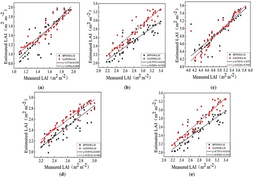
Table 9. Accuracy evaluation of the neural network model.

Model	Growth Stage	R^2	RMSE	Model	Growth Stage	R^2	RMSE
GANNM	Jointing	0.8223	0.2130	BPNNM	Jointing	0.7865	0.3021
	Booting	0.8924	0.1872		Booting	0.7897	0.2258
	Heading	0.9021	0.1675		Heading	0.7672	0.3245
	Filling	0.8121	0.1823		Filling	0.7897	0.2855
	Maturing	0.8536	0.1814		Maturing	0.7444	0.3542

As can be seen from Figure 6 and Table 9, GANNM achieved the best inversion of winter wheat LAI at the heading stage; the R² was 0.9021, and RMSE was 0.1675. The inversion accuracy decreased in the order of booting (R² = 0.8924 and RMSE = 0.1872), maturing (R² = 0.8536 and RMSE = 0.1814), jointing (R² = 0.8223 and RMSE = 0.2130), and filling stage (R² = 0.8121 and RMSE = 0.1823). BPNNM realized the best inversion of winter wheat LAI at the booting stage; the R² was 0.8074, and RMSE was 0.2258. The inversion accuracy decreased in the order of filling (R² = 0.7897 and RMSE = 0.2855), jointing (R² = 0.7865 and RMSE = 0.3021), heading (R² = 0.7672 and RMSE = 0.3245), and maturing stage (R² = 0.7444 and RMSE = 0.3542). In summary, the nonlinear mapping ability, self-learning and self-adaptive ability, generalization ability, and fault tolerance ability of GANNM enabled it to generate good inversion results for solving the complex relationship model of winter wheat LAI inversion in five growth stages and to estimate winter wheat LAI quickly and accurately in five growth stages.

3.4. GANNM verification

To verify the reliability of the LAI inversion model, the LAI value obtained by GANNM inversion was studied, and the measured LAI was taken as the true value. Regression analysis was conducted between the remaining 40 true values, other than the modeling samples and the LAI value inverted by GANNM, to obtain the correlation between the LAI inversion value and the true value in each growth stage (Figure 7).

Figure 7. The GANNM model and LAI verification analysis. (a–e) are from the jointing, booting, heading, filling, and maturing stages, respectively.

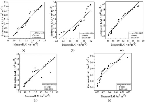
As can be seen from Figure 7, the R² between the LAI of the five growth stages of winter wheat inverted by GANNM and the measured LAI was 0.8736, 0.8169, 0.8863, 0.8723, and 0.8310, respectively, and the RMSE was 0.3845, 0.4529, 0.4135, 0.3998, and 0.3611, respectively. Comprehensive analysis of Figure 3 shows that although the correlation of each growth stage was different, the R² was above 0.87 and the maximum RMSE was 0.4529, indicating that the LAI inversion of winter wheat in five growth stages by GANNM reflected the growth and changes in winter wheat with preferable inversion results.

3.5. GANNM cross validation

To further verify the accuracy of the inversion model, the LAI images of five typical growth stages of winter wheat obtained by inversion were resampled to 1 km, and 100 points were randomly selected. The LAI (GF-3 LAI) of five growth stages of winter wheat based on GF-3 remote sensing images and MODIS LAI products (MOD15A2) of corresponding phases were regressed and analyzed to obtain the correlation of five growth stages of winter wheat, as shown in Figure 8.

Figure 8. Correlation analysis between GF-3 LAI and MODIS LAI. (a–e) are from the jointing, booting, heading, filling, and maturing stages, respectively.

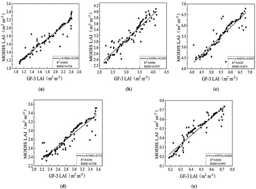
As can be seen from Figure 8, MODIS LAI and GF-3 LAI had a strong correlation in the five typical growth stages of winter wheat. The correlation between the two was strongest at the jointing stage (R² = 0.8842 and RMSE = 0.3756), followed by the maturing (R² = 0.8524 and RMSE = 0.3995), booting (R² = 0.8444 and RMSE = 0.3579), filling (R² = 0.8356 and RMSE = 0.3788), and heading stage (R² = 0.8229 and RMSE = 0.4531). According to the statistics of the mean values of 100 sampling points, the mean values of GF-3 LAI and MODIS LAI at the jointing stage were 1.53 and 1.35, respectively. At the booting stage, the mean value of GF-3 LAI was 2.72, and the mean value of MODIS LAI was 2.66. The mean LAI value of GF-3 and MODIS at the heading stage was 3.79 and 3.51, respectively. The mean value of GF-3 LAI was 2.35 and the mean value of MODIS LAI was 2.09 at the filling stage. The mean LAI value of GF-3 and MODIS at the maturing stage were 1.22 and 1.08, respectively. The MODIS LAI of winter wheat in five growth stages was lower than GF-3 LAI to varying degrees, which was related to the low spatial resolution of MODIS and serious pixel mixing. This phenomenon of over- or underestimation has also been confirmed by other scholars (Li et al. 2021).

3.6. Mapping of LAI inversion by GANNM

On the basis of the verified reliability of each inversion model, GANNM was employed to generate winter wheat LAI spatial distribution maps in five growth stages, as shown in Figure 9.

Figure 9. LAI images inverted by GANNM. (a–e) are from the jointing, booting, heading, filling, and maturing stages, respectively. (f–j) are the enlarged image from the (a–e) area.

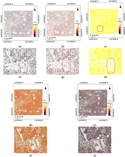
The actual investigation revealed that winter wheat in the test region was mainly distributed in the central and southeastern areas. As shown in Figure 9 (a–e), the non-vegetated area is white, and the vegetated area is colored. The LAI value of winter wheat at the jointing stage was between 1 and 2, with an average value of 1.53. The larger LAI of winter wheat was mainly concentrated in the southeast area, which was caused by the earlier sowing time of winter wheat in this region. The LAI values of winter wheat at the booting, heading, and filling stages were 2.5–3.5, 3.8–4.5, and 2–3, respectively, with average values of 2.72, 3.79, and 2.35, respectively. Among them, the larger LAI was mainly concentrated in the southeast area, while the LAI of winter wheat in the northwest area was generally smaller. The LAI value of winter wheat in the maturing stage was between 0 and 1.5, and the average value was 1.22. Among them, the LAI of winter wheat was mainly concentrated in the south. As shown in Figure 9 (f–j), at the jointing and booting stages, due to the low coverage of winter wheat, there were local abnormal values in the LAI inversion results of GANNM. The inversion results of other growth periods were basically consistent with the growth status of winter wheat LAI. In summary, the LAI of winter wheat in the five growth stages inverted by GANNM was basically consistent with the local winter wheat growth status and the local situation.

4. Conclusions

In this paper, based on GF-3 SAR images and GF-1 WFV images, GANNM was exploited to invert the LAI of winter wheat in the Xiangfu District in the east of Kaifeng City, Henan Province, during the whole growth cycle, and the measured LAI data was used to verify it. The experimental results showed that the regression model of MNDVI and LAI was better than the other models when the five optical and microwave polarization decomposition vegetation index models were used to invert the winter wheat LAI in the whole growth cycle. The proposed method was simple and easy to generalize, which effectively overcame the problem of saturation of optical remote sensing information when LAI was large. However, it ignored the complex transmission process of photons in the vegetation canopy and had poor portability. Five kinds of optical and microwave polarization decomposition vegetation indices (MNDVI, MSAVI, MEVI, MEVI₂, MMSAVI) were significantly correlated with the measured LAI at P < 0.01, which can be used as the input factor of the neural network model. The fitting accuracy of the backscattering coefficient (${\sigma }_0$) extracted by MWCM under HV polarization with LAI was higher than that of HH and VV polarizations. The accuracy of LAI inversion by MWCM was higher than that by WCM. Therefore, three kinds of backscattering coefficients (${\sigma }_0$) and LAI data inverted by MWCM can be used as input factors of the neural network model together with five kinds of optical and microwave polarization decomposition vegetation indices. GANNM had higher fitting accuracy than BPNNM in inverting the LAI of winter wheat in the whole growth cycle. The R² was higher than 0.8, and RMSE was lower than 0.22, which corresponds with the actual growth status of local winter wheat.

Acknowledgement

We appreciate the detailed suggestions and comments from the anonymous reviewers. The authors thank by Guosheng Cai, Yushi Zhou, and Qinggang Zhang for the assistance with flight tests, and the other members of the Institute of Remote Sensing and Surveying and Mapping for assistance with LAI and $M_S$ measurements.

Data availability statement

The code used in this study are available by contacting the corresponding author.

Disclosure statement

No potential conflict of interest was reported by the author(s).

Additional information

Funding

This research was funded by 2016 National Key Research and Development Plan (grant number 2016YFC0803103), Research on Key Technology of Agricultural Remote Sensing Monitoring (grant number 12210243), and Henan Provincial University Innovation Team Support Plan (grant number 14IRTSTHN026).

References

- Abadi, M. Q. H., S. Rahmati, A. Sharifi, and M. Ahmadi. 2021. “HSSAGA: Designation and Scheduling of Nurses for Taking Care of COVID-19 Patients Using Novel Method of Hybrid Salp Swarm Algorithm and Genetic Algorithm.” Applied Soft Computing 108: 107449.
- Alhijawi, B., and A. Awajan. 2021. “Novel Textual Entailment Technique for the Arabic Language Using Genetic Algorithm.” Computer Speech & Language 68: 101194.
- Amar, J., and K. Nagase. 2021. “Genetic-Algorithm-Based Global Design Optimization of Tree-Type Robotic Systems Involving Exponential Coordinates.” Mechanical Systems and Signal Processing 156 (8): 107461.
- Amin, E., J. Verrelst, J. P. Rivera-Caicedo, L. Pipia, A. Ruiz-Verdú, and J. Moreno. 2021. “Prototyping Sentinel-2 Green LAI and Brown LAI Products for Cropland Monitoring.” Remote Sensing of Environment 255: 112168.
- Attema, E. P. W., and F. T. Ulaby. 1978. “Vegetation Modeled as a Water Cloud.” Radio Science 13: 357–364.
- Carrabs, F. 2021. “A Biased Random-key Genetic Algorithm for the set Orienteering Problem.” European Journal of Operational Research 292: 830–854.
- Deng, Z., M. Yan, and X. Xiao. 2021. “An Early Risk Warning of Cross-Border e-Commerce Using BP Neural Network.” Mobile Information Systems 2021: 1–8.
- Gómez-Candón, D., J. Bellvert, and C. Royo. 2021. “Performance of the Two-Source Energy Balance (TSEB) Model as a Tool for Monitoring the Response of Durum Wheat to Drought by High-Throughput Field Phenotyping.” Frontiers in Plant Science 12: 658357.
- Graham, A. J., and R. Harris. 2002. “Estimating Crop and Waveband Specifific Water Cloud Model Parameters Using a Theoretical Backscatter Model.” International Journal of Remote Sensing 23 (23): 5129–5133.
- Inoue, Y., T. Kurosu, H. Maeno, S. Uratsuka, T. Kozu, K. Dabrowska-Zielinska, and J. Qi. 2002. “Season-long Daily Measurements of Multifrequency (Ka, Ku, X, C, and L) and Full-Polarization Backscatter Signatures Over Paddy Rice Field and Their Relationship with Biological Variables.” Remote Sensing of Environment 81: 194–204.
- Jafari, M., and A. Keshavarz. 2021. “Improving CERES-Wheat Yield Forecasts by Assimilating Dynamic Landsat-Based Leaf Area Index: A Case Study in Iran.” Journal of the Indian Society of Remote Sensing: 1–14. Published online.
- Katsuhama, N., M. Imai, N. Naruse, and Y. Takahashi. 2018. “Discrimination of Areas Infected with Coffee Leaf Rust Using a Vegetation Index.” Remote Sensing Letters 9: 1186–1194.
- Kweon, S. K., and O. H. Yisok. 2015. “A Modified Water-Cloud Model with Leaf Angle Parameters for Microwave Backscattering from Agricultural Fields.” IEEE Transactions on Geoscience & Remote Sensing 53: 2802–2809.
- Le Maire, G., C. Marsden, Y. Nouvellon, J.-L. Stape, and F. Ponzoni. 2012. “Calibration of a Species-Specific Spectral Vegetation Index for Leaf Area Index (LAI) Monitoring: Example with MODIS Reflectance Time-Series on Eucalyptus Plantations.” Remote Sensing 4: 3766–3780.
- Li, X., H. Du, G. Zhou, F. Mao, M. Zhang, N. Han, W. Fan, et al. 2021. “Phenology Estimation of Subtropical Bamboo Forests Based on Assimilated MODIS LAI Time Series Data.” ISPRS Journal of Photogrammetry and Remote Sensing 173 (6): 262–277 .
- Li, F., S. Fang, Y. Shen, and D. Wang. 2021. “Research on Graphene/Silicon Pressure Sensor Array Based on Backpropagation Neural Network.” Electron. Letter 57: 419–421 .
- Liao, C., J. Wang, J. Shang, X. Huang, J. Liu, and T. Huffman. 2018. “Sensitivity Study of Radarsat-2 Polarimetric SAR to Crop Height and Fractional Vegetation Cover of Corn and Wheat.” International Journal of Remote Sensing 39 (5-6): 1475–1490.
- Niu, C., H. Zhang, W. Liu, R. Li, and T. Hu. 2021. “Using a Fully Polarimetric SAR to Detect Landslide in Complex Surroundings: Case Study of 2015 Shenzhen Landslide.” ISPRS Journal of Photogrammetry and Remote Sensing 174: 56–67.
- Prévot, L., I. Champion, and G. Guyot. 1993. “Estimating Surface Soil Moisture and Leaf Area Index of a Wheat Canopy Using a Dual-Frequency (C and X Bands) Scatterometer.” Remote Sensing of Environment 46: 331–339.
- Ren, Z., Y. Du, X. He, R. Pu, H. Zheng, and H. Hu. 2018. “Spatiotemporal Pattern of Urban Forest Leaf Area Index in Response to Rapid Urbanization and Urban Greening.” Journal of Forestry Research 29: 785–796.
- Ulaby, F. T., C. T. Allen, G. E. Iii, and E. Kanemasu. 1984. “Relating the Microwave Backscattering Coefficient to Leaf Area Index.” Remote Sensing of Environment 14: 113–133.
- Wali, E., M. Tasumi, and M. Moriyama. 2020. “Combination of Linear Regression Lines to Understand the Response of Sentinel-1 Dual Polarization SAR Data with Crop Phenology—Case Study in Miyazaki, Japan.” Remote Sensing 12: 189.
- Wang, L., Z. Liu, J. Guo, Y. Wang, J. Ma, S. Yu, P. Yu, and L. Xu. 2021. “Estimate Canopy Transpiration in Larch Plantations via the Interactions among Reference Evapotranspiration, Leaf Area Index, and Soil Moisture.” Forest Ecology and Management 481: 118749.
- Wang, Y., and D. Qing. 2021. “Model Predictive Control of Nonlinear System Based on GA-RBP Neural Network and Improved Gradient Descent Method.” Complexity 2021 (3): 1–14.
- Wang, Y., Y. Wang, Z. Li, P. Yu, and X. Han. 2020. “Interannual Variation of Transpiration and its Modeling of a Larch Plantation in Semiarid Northwest China.” Forests 11 (12): 1303.
- Xu, H. 1996. “Monitoring Leaf Area of Sugar Beet Using ERS-1 SAR Data.” International Journal of Remote Sensing 17: 3401–3410.
- Xu, J., F. Chen, and C. Deng. 2021. “Design and Analysis of a Novel Multi-Sectioned Compound Parabolic Concentrator with Multi-Objective Genetic Algorithm.” Energy 225: 120216.
- Xu, T., J. Liao, G. Shen, J. Wang, X. Yang, and M. Wang. 2016. “Estimation of Wetland Vegetation LAI in the Poyang Lake Area Using GF-1 and Radarsat-2 Data (in Chinese).” Journal of Infrared and Millimeter Waves 35: 332–340.
- Xu, X. O., A. Marino, L. Li, X. Xu, A. Marino, and L. Li. 2011. “Biomass Related Parameter Retrieving from Quad-Pol Images Based on Freeman-Durden Decomposition.” In Proceedings of 2011 IEEE International Geoscience and Remote Sensing Symposium, Vancouver, BC, Canada, July. doi:10.1109/igarss.2011.6049005.
- Yadav, V. P., R. Prasad, and R. Bala. 2021. “Leaf Area Index Estimation of Wheat Crop Using Modified Water Cloud Model from the Time-Series SAR and Optical Satellite Data.” Geocarto International 36: 791–802.
- Yang, Z., K. Li, Y. Shao, B. Brisco, and L. Liu. 2016. “Estimation of Paddy Rice Variables with a Modified Water Cloud Model and Improved Polarimetric Decomposition Using Multi-Temporal RADARSAT-2 Images.” Remote Sensing 8: 878.
- Zhang, L. L., Q. Y. Meng, S. Yao, Q. Wang, J. Zeng, S. Zhao, and J. W. Ma. 2018. “Soil Moisture Retrieval from the Chinese GF-3 Satellite and Optical Data Over Agricultural Fields.” Sensors 18 (8): 2675.
- Zhao, Y., S. Dong, F. Jiang, and A. Incecik. 2021a. “Mooring Tension Prediction Based on BP Neural Network for Semi-Submersible Platform.” Ocean Engineering 223 (4): 108714 .
- Zhao, Y., J. Liu, J. Ma, and L. Wu. 2021b. “Multi-branch Cable Harness Layout Design Based on Genetic Algorithm with Probabilistic Roadmap Method.” Chinese Journal of Mechanical Engineering 34 (1 ).