Reopen schools safely: simulating COVID-19 transmission on campus with a contact network agent-based model

ABSTRACT

As the COVID-19 vaccination has been quickly rolling out around the globe, the evaluation of the effects of vaccinating populations for the safe reopening of schools has become a focal point for educators, decision-makers, and the general public. Within this context, we develop a contact network agent-based model (CN-ABM) to simulate on-campus disease transmission scenarios. The CN-ABM establishes contact networks for agents based on their daily activity patterns, evaluates the agents’ health status change in different activity environments, and then simulates the epidemic curve. By applying the model to a real-world campus environment, we identify how different community risk levels, teaching modalities, and vaccination rates would shape the epidemic curve. The results show that without vaccination, retaining under 50% of on-campus students can largely flatten the curve, and having 25% on-campus students can achieve the best result (peak value < 1%). With vaccination, having a maximum of 75% on-campus students and at least a 45% vaccination rate can suppress the curve, and a 65% vaccination rate can achieve the best result. The developed CN-ABM can be employed to assist local government and school officials with developing proactive intervention strategies to safely reopen schools.

KEYWORDS:

• COVID-19
• contact network
• vaccination
• agent-based modeling
• school

1. Introduction

Learning environments such as schools are characterized by frequent social gatherings and extensive interpersonal interactions, making them ideal breeding grounds for viruses (Chao, Halloran, and Longini 2010; Gog et al. 2014). Due to the highly contagious nature of the Coronavirus Disease 2019 (COVID-19), school closures and pedagogical transitions from in-person to remote learning were widely implemented to control the spread of the disease (Viner et al. 2020). The World Health Organization (WHO) estimated that about 90% of the world’s students, which were more than 1.5 billion children and young adults, were affected by school closures (WHO 2020a). The cascading impacts of such school closures included reduced work efficiency (Li et al. 2020), lack of educational resources (UNESCO 2020), and mental health issues caused by social isolation (Brooks et al. 2020). Burdened with these grave concerns and the political pressure to revive the global economy, governments of many countries laid out plans or enacted policies to reopen schools. However, these reopening plans and their implementation often lacked scientific evidence to weigh the potential benefits versus the consequences to public health. For example, a national survey of more than 1,900 universities and colleges in the United States revealed over 397,000 COVID-19 cases and 90 deaths were the results of school reopenings (Cai et al. 2020). This poignant reality signifies that it is of utmost significance to employ rigorous measures to evaluate the health risk for school reopening (Mallapaty 2020).

Existing studies have used process-based dynamic epidemic models, primarily the Susceptible-Exposed-Infective-Recovered (SEIR) model and its variations, to simulate the potential for COVID-19 outbreaks (Chen et al. 2021; Read et al. 2021; Wu, Leung, and Leung 2020; Zeng et al. 2020; Yu et al. 2021). Although these models can project the spread of COVID-19 under different social distancing scenarios, they cannot be easily implemented in a school environment without major modification. First and foremost, existing studies and models have been mainly focused on macro-scale assessments with aggregate administrative units (e.g. counties, census tracts). As such, the ability to model the intricacy of the disease transmission processes at the individual scale, known as the micro-scale, which plays a vital role in determining the likelihood of virus spread in a school environment has been absent. Second, existing studies mostly employ deterministic models without considering the stochastic transmission process of diseases, such as the infection rates in different human activity environments (e.g. indoors or outdoors environments). These uncertainties at the micro-scale can dictate the likelihood of outbreaks when schools reopen. To date, existing micro-scale predictive models, especially those applicable to schools, are considerably lacking.

In this paper, we propose a contact network agent-based model (CN-ABM) to simulate the COVID-19 transmission processes in a school environment. In the model, we define on-campus students as potential disease-spreading agents and construct a fine-grained dynamic contact network between agents based on their daily activity patterns and movement trajectories. Then, we have employed the model to simulate on-campus transmission scenarios under WHO’s guidelines for school reopening (WHO 2020b). Specifically, we have evaluated how the epidemic curve (epi curve) is shaped by different community risk levels, teaching modalities, and vaccination rates. It is hoped that the proposed model can help to shape school reopening strategies amid the ongoing COVID-19 vaccination practices.

This paper is organized as follows. Section 2 introduces the methods, including the conceptual framework and the proposed simulation model. Section 3 applies the model to a school environment and derives the results, including the epi curve and the transmission chain. Section 4 performs a sensitivity analysis of the model by incorporating different vaccination rates, discusses the model’s public health implications, and also presents the limitations. Finally, Section 5 concludes the study with future directions.

2. Methods

2.1. Conceptualizing contact network

An agent-based model (ABM) is a micro-scale model that simulates the synchronous interactions of agents based on pre-defined rules (Wooldridge 2009). ABMs have been integrated into social network science to enhance the understanding of human behaviors (Chen et al. 2012). In a network-based ABM, each agent can be represented as a node, which interacts with other agents under predefined behavioral assumptions in an abstracted interaction network (Cardinot et al. 2019). Recently, network-based ABMs have received elevated attention in near real-time genome sequencing of the SARS-CoV-2 virus (Rockett et al. 2020). Several network-based ABMs have been proposed to simulate COVID-19 transmission between countries and regions with the temporal unit being a day (Kerr et al. 2021; Hinch et al. 2021; Gomez et al. 2021; Cuevas 2020; Silva et al. 2020). Their applications to the COVID-19 transmission on the community scale (e.g. schools) with a fine temporal unit (e.g. one minute) are relatively lacking.

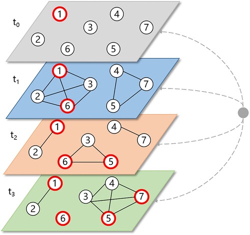
The transmission process of the SARS-CoV-2 virus can be regarded as the transition of an individual's health status via interactions with infectious agents (Chang et al. 2020). This process is illustrated by Figure 1, where an agent’s health status could change if the agent’s contact network includes an infectious agent. Additionally, the internal transmission process inside a school can be influenced by the community spread beyond the school environment (Gemmetto, Barrat, and Cattuto 2014). Therefore, we incorporated the community risk as an external node into the contact network, meaning that each agent can become infectious at a given probability even without contacting other internal agents (Figure 1).

Figure 1. Schematic illustration of the contact network. Red nodes are infectious agents; lines are interactions between agents via their close contact at a time point. An external node is introduced to represent the community risk.

To construct the contact network, all agents’ daily activity patterns, including their movement trajectories, locations of stay in an activity environment (e.g. a dining hall, a residential building, a classroom), and periods of stay, must be acquired. Deriving these activity patterns for all agents is a prerequisite for building the contact network at each point in time. This process in our case study is detailed in Appendix 1.

2.2. Infection phases

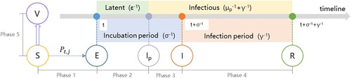
Based on the classical SEIR model, an agent’s health status in an infection cycle can be divided into four overarching phases: susceptible (S), exposed (E), infectious (I), and recovered (R). The transition of the health status, reflecting the disease progression, is key to simulating the virus spread. Based on another school modeling study (Di Domenico et al. 2021) and the successive vaccination stage (Huang et al. 2021), we introduced six heath statuses to illustrate a complete infection cycle, including susceptible (S), exposed (E), pre-symptomatic (I_p), infected (I), recovered/removed (R), and vaccinated (V). These six health statuses constitute five infection phases, as shown in Figure 2.

Figure 2. Schematic illustration of an infection cycle with the change of an agent’s health status (E = exposed, I_p = pre-symptomatic, I = infected, R = recovered, and V = vaccinated).

The transition of an agent’s health status at each infection phase is articulated as follows:

Phase 1 (S → E): the probability of an agent transitioning from S to E in an activity environment j at time t is P_t,j. This probability is dependent on both the internal infection probability Φ_t,j and the external (community) infection probability Ψ, as shown in Equation (1). An agent’s internal infection probability Φ_t,j in activity environment j at time t is shown in Equation (2). An agent’s external infection probability Ψ is a ratio of the external infection rate in the community p_c to the agent’s health level H, as shown in Equation (3). (1) $P_{t,j}=1-\left(1-{\mathrm{\Phi }}_{t,j}\right)\left(1-\mathrm{\Psi }\right)$(1) (2) ${\mathrm{\Phi }}_{t,j}={\displaystyle \frac{1-{\left(1-K{p}_j\right)}^{m_t}{\left(1-p_j\right)}^{n_t}}{H}}$(2) (3) $\mathrm{\Psi }={\displaystyle \frac{p_c}{H}}$(3)

Notation:

H: agent’s health level;

K: decay coefficient for the infection rate of an I_p-status agent;

m_t: number of I_p-status neighbors in an agent’s contact network at time t;

n_t: number of I-status neighbors in an agent’s contact network at time t;

p_c: external infection rate in the community;

p_j: infection rate in activity environment j;

P_t,j: probability of an agent transitioning from S to E in activity environment j at time t;

Φ_t,j: internal infection probability;

Ψ: external infection probability.

Phase 2 (E → I_p): an E-status agent transitions to the I_p-status after a latent period (ϵ⁻¹). During this phase (t through t + ϵ⁻¹), the agent is not infectious.

Phase 3 (I_p → I): an I_p-status agent transitions to the I-status after the prodromal period (μ_p⁻¹); and the duration from E to I is the incubation period σ⁻¹. During this phase (t + ϵ⁻¹ through t + σ⁻¹), an I_p-status agent infects all S-status neighbors at an infection rate Kp_j if they are within the same contact network.

Phase 4 (I → R): an I-status agent transitions to R-status after the infection period (γ⁻¹). During this phase (t + σ⁻¹ through t + σ⁻¹ + γ⁻¹), the I-status agent infects S-status neighbors in its contact network at the infection rate p_j.

Phase 5 (S → V): an S-status agent transitions to V-status when it is vaccinated. A V-status agent is not infectious and cannot be infected. The number of S-status agents is determined by the initial number of S-status agents S₀ and the immunized agents αvS₀, where v is the vaccination rate and α is the vaccine efficacy (Kim, Marks, and Clemens 2021), as is shown in Equation (4). (4) $S=\left(1-\alpha v\right)S_0$(4) The parameters in Figure 2 and Equations (1) through (4) are derived from existing epidemiological parameters, as shown in Table 1.

Table 1. Epidemiological parameters used in the simulation model.

Parameter	Explanation	Value	Reference
σ^−1	Incubation period	σ^−1∼lognormal (1.6, 0.5)∩σ^−1∈[2, 14] days	(McAloon et al. 2020)
μp^−1	Prodromal period	2 days	(Kim et al. 2020)
ϵ^−1	Latent period	σ^−1 - μp^−1	–
γ^−1	Infection period	γ^−1∼lognormal (2.05, 0.25)	(Wölfel et al. 2020)
K	Decay coefficient for the infection rate of an Ip-status agent	1/3	(Chen et al. 2020)
pj	Internal infection rate in an activity environment j	Dining hall: 3.03e^−4/min; residential building: 1.74e^−4/min; lecture hall (including library): 3.30e^−5/min	(Chen et al. 2020)
pc	External infection rate in the community	9.5e^−8/min	(Gemmetto, Barrat, and Cattuto 2014)
H	Agent’s health level	1/H∼normal(1, 0.1)	(Yang and Atkinson 2008)
α	Vaccine efficacy	80%	(WHO 2021)

The agent’s health level H reflects the differences in personal health concerning the likelihood of infection (Yang and Atkinson 2008). It is given as 1/H for each agent based on a normal distribution with a mean value of 1 and a standard deviation of 0.1. The decay coefficient K represents the infection rate of an I_p-status agent compared to that of an I-status agent, as pre-symptomatic cases have been proven to have a lower transmission risk than infected cases (Wu 2020). The number of I_p-status neighbors m_t and I-status neighbors n_t in an agent’s contact network at time t are not fixed values, which are determined by the actual number of agents at the same activity location at time t.

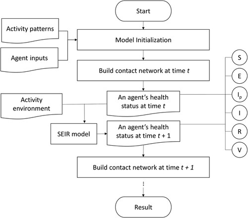
The workflow for the ABM simulation is demonstrated by Figure 3. We term this proposed model the contact network agent-based model (CN-ABM).

Figure 3. Workflow of the CN-ABM model for simulating COVID-19 transmission in a school environment.

3. Results

We built the proposed CN-ABM model in MATLAB R2019a. The code of the model can be accessed from GitHub (https://github.com/xic19022/cnabm). Our computational environment was as follows: CPU Intel(R) Xeon(R) E5-2620 (8-core/2.10 GHz) and RAM of 64GB. Our model was applied using a real-world learning environment with different environmental settings. The results of these modeling applications are discussed in detail in the sub-sections below.

3.1. Model initialization

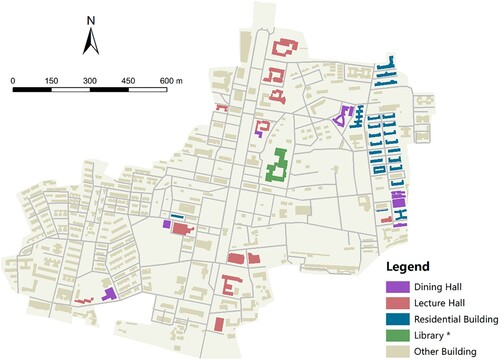
Our study area was a university campus located in Southern China. We derived the building footprints and the road networks on campus using the Baidu Map application programming interface (API) (https://lbsyun.baidu.com/), as shown in Figure 4. The shortest network distance between every two buildings was also derived by the API and was converted to walking time (in minutes) based on the average human walking speed (i.e. 5 km per hour). To initialize the simulation, we generated 10,000 agents in the starting scenario (t = 0) and introduced 0.1% pre-symptomatic cases among them. We allocated these agents into the residential buildings proportional to the building capacities across the campus. Then, each agent was assumed to follow a similar activity pattern but select the activity location of the same type randomly. It should be noted that this activity pattern was assumed to be on a weekday, whereas weekends and holidays were not considered in our simulation (see details in Appendix 1). The contact network at each point in time was then built for all agents over the simulation period.

Figure 4. Building footprints of the campus in the study area. *The library is considered a lecture hall in the model simulation; other buildings (e.g. administrative buildings) are excluded from the simulation.

In the first analysis, we established twelve school reopening scenarios based on different teaching modalities (i.e. the composition of on-campus and distance-learning students) and community risk levels (i.e. external infection rates), as shown in Table 2. The distance-learning students were not present on campus and were thus excluded from the simulation. We did not consider the vaccination phase (i.e. Phase 5 in Figure 2) in the initial analysis, as it is discussed in the following section. For each scenario, we performed the simulation for the first twenty-five weeks of an outbreak at a one-minute timestamp. We also repeated each simulation five times to account for the stochastic nature of the disease transmission.

Table 2. Twelve school reopening scenarios based on different community risk levels and teaching modalities.

	Student composition (% of distance-learning)
Community risk level (external infection rate)	In-class (0%)	Mostly in-class (25%)	Hybrid (50%)	Mostly online (75%)
No risk (0)	N-S0	N-S25	N-S50	N-S75
Low risk (pc)*	L-S0	L-S25	L-S50	L-S75
High risk (5x pc)	H-S0	H-S25	H-S50	H-S75

* p_c is 9.5e⁻⁸/min (Gemmetto, Barrat, and Cattuto 2014).

3.2. Simulated epi curves

Figure 5 presents the simulation results in terms of the epi curves (i.e. the percentage of active infectious agents over time) under the twelve school reopening scenarios. The results reveal two important epidemiological patterns. First, our results demonstrate that teaching modality largely affects the epi curve. For example, on a low community risk level, when all students are on campus (L-S0), the peak value of the epi curve or the maximum percentage of infections is 22.38% (the blue curve, Figure 5b). Then, reducing the on-campus students by 25% (L-S25), 50% (L-S50), and 75% (L-S75) will considerably flatten the curve, where the peak values are 12.40%, 1.64%, and 0.40%, respectively (Figure 5b). Second, the influence of the community risk on the transmission is moderate, and a high community risk advances the emergence of the peak time. For example, under the same modality of ‘mostly in-class’ (red curves in Figure 5) but different community risk levels, the peaks of the epi curves emerge on the 95th day (N-S25, no risk, Figure 5a), the 83rd day (L-S25, low risk, Figure 5b), and the 64th day (H-S25, high risk, Figure 5c), respectively. The statistics of the epi curves, including the peak height and the peak day, are given in Table 3. The peak height and peak reduction rate in Table 3 are visualized in Figure 6.

Figure 5. Simulation results under different community risks: (a) no risk, (b) low risk, and (c) high risk. Curves in different colors represent different teaching modalities; the Y-axis is the simulated active infectious cases as a percentage of the total agents (%); the X-axis is the day of simulation.

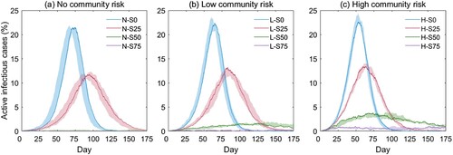
Figure 6. Simulated peak heights and peak reduction rates under different community risks: (a) no risk, (b) low risk, and (c) high risk. Different-colored bars represent different teaching modalities; yellow curves represent peak reduction rates; the left Y-axis is the peak height (%) of active infectious cases; the right Y-axis is the peak reduction rate (%).

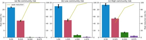
Table 3. Statistics of the simulation results under the twelve school reopening scenarios.

Scenario	Peak height (min, max)*	Peak reduction rate**	Peak day (min, max)*
N-S0	21.49% (21.30%, 22.02%)	–	74 (67, 75)
N-S25	12.03% (11.29%, 12.40%)	44.02%	95 (84, 96)
N-S50	0.14% (0.12%, 0.36%)	99.35%	11 (8, 160)***
N-S75	0.12% (0.12%, 0.16%)	99.44%	6 (5, 8)***
L-S0	22.38% (21.18%, 23.77%)	–	65 (60, 67)
L-S25	12.40% (11.60%, 13.23%)	44.59%	83 (78, 87)
L-S50	1.64% (1.56%, 2.02%)	92.67%	125 (122, 145)
L-S75	0.40% (0.32%, 0.48%)	98.21%	146 (111, 169)
H-S0	23.38% (22.66%, 24.46%)	–	53 (52, 55)
H-S25	13.52% (13.41%, 14.11%)	42.17%	64 (63, 70)
H-S50	3.64% (3.10%, 4.00%)	84.43%	74 (63, 91)
H-S75	1.12% (0.92%, 1.16%)	95.21%	152 (101, 166)

*Derived from the median of the five repeated simulations for each scenario. The peak day is rounded.

**Defined as the current peak height relative to the peak height in the corresponding baseline scenario (S0).

***The peak emerges early, as the outbreak is not prominent.

3.3. Transmission chain

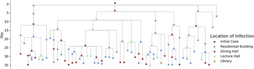
The proposed CN-ABM model is capable of projecting COVID-19 epi curves for a potential outbreak scenario. More importantly, it can be used to infer the transmission chain. Figure 7 illustrates an example of an inferred transmission chain for an infectious disease agent (i.e. the initial case) over the first 35 days of a disease’s progression. Specifically, the figure shows that under the N-S0 scenario, the initial case can affect 104 other agents in the person’s contact network, while most of the infections (58.65%) occur in residential buildings (i.e. 61 agents in the scenario’s residential building, 30 agents in the dining hall, 12 agents in the lecture hall, and 1 agent in the library). This result is consistent with the epidemiological findings that most of the COVID-19 transmissions arise in residential units due to unavoidable interpersonal contact (Song et al. 2020). Thus, this derived transmission chain corroborates the necessity of minimizing room-sharing and reducing the capacity of residential buildings to contain the virus spread. Constructing such a transmission chain can help track where and when the transmissions take place and can provide evidence to formulate proactive intervention strategies in high-risk activity environments (Kelvin and Halperin 2020).

Figure 7. The transmission chain of an agent in the first 35 days of the disease progression under the N-S0 scenario.

4. Discussion

4.1. How does vaccination shape the epi curve?

While phases of vaccination are rolling out in countries and regions around the globe, there has been a lack of understanding about how the vaccination process shapes the epi curves at the community level (Kim, Marks, and Clemens 2021). In the second analysis, we evaluated the health outcomes under fifteen school reopening scenarios based on the combinations of community risk levels and vaccination rates (Table 4). The vaccination phase (Phase 5 in Figure 2) presumes that when a portion of S-status agents convert to V-status, they become immune to the virus and are excluded from the infection cycle. To facilitate the bi-variate analysis, we assumed all agents were in-class (0% distance-learning) in the model initialization. The simulation results in terms of the epi curves are given in Figure 8.

Figure 8. Simulation results under different community risks: (a) no risk, (b) low risk, and (c) high risk. Different-colored curves represent different vaccination rates; the Y-axis is the simulated active infectious cases as a percentage of the total agents (%); the X-axis is the day of simulation.

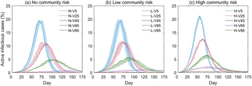
Table 4. Fifteen school reopening scenarios based on different community risks and vaccination rates.

Community risk level (external infection rate)	Vaccination rate (% of vaccinated agents)
	5%	25%	45%	65%	85%
No risk (0)	N-V5	N-V25	N-V45	N-V65	N-V85
Low risk (pc)*	L-V5	L-V25	L-V45	L-V65	L-V85
High risk (5x pc)	H-V5	H-V25	H-V45	H-V65	H-V85

* p_c is 9.5e⁻⁸/min (Gemmetto, Barrat, and Cattuto 2014).

Figure 8 reveals two important epidemic patterns. First, the vaccination rate is the primary parameter shaping the epi curve. For example, on a low community risk level, high vaccination rates will largely flatten the curve—the vaccination rates of 5% (L-V5), 25% (L-V25), 45% (L-V45), 65% (L-V65), and 85% (L-85) yield a peak value of 19.62%, 11.73%, 5.23%, 1.14%, and 0.20%, respectively (Figure 8b). Second, similar to the results in Section 3.2, the influence of the community risk is moderate, and a high community risk slightly advances the emergence of the peak. For example, at the vaccination rate of 45% (the green curves in Figure 8), the peaks of the epi curves emerge on the 102nd day (N-V45, no risk, Figure 8a), the 90th day (L-V45, low-risk, Figure 8b), and the 71st day (H-V45, high risk, Figure 8c), respectively.

Our third analysis simulates the health outcome resulting from different teaching modalities and vaccination rates. Since distance learning and vaccination are both preventive measures to contain the disease transmission, it is expected that combining these two measures will mitigate the likelihood of outbreaks to the largest extent. Thus, we designed twenty school reopening scenarios by combining different teaching modalities and vaccination rates (Table 5), whereas all scenarios are predicated on a low community risk level (p_c = 9.5e⁻⁸/min). The simulated epi curves are given in Figure 9.

Figure 9. Simulation results with different teaching modalities: (a) in-class, (b) mostly in-class, (c) hybrid, and (d) mostly online. Different-colored curves represent different vaccination rates; the Y-axis is the simulated active infectious cases as a percentage of the total agents (%); the X-axis is the day of simulation.

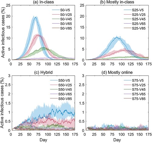
Table 5. Twenty school reopening scenarios based on different teaching modalities and vaccination rates.

Student composition (% of distance-learning)	Vaccination rate
	5%	25%	45%	65%	85%
In-class (0%)	S0-V5	S0-V25	S0-V45	S0-V65	S0-V85
Mostly in-class (25%)	S25-V5	S25-V25	S25-V45	S25-V65	S25-V85
Hybrid (50%)	S50-V5	S50-V25	S50-V45	S50-V65	S50-V85
Mostly online (75%)	S75-V5	S75-V25	S75-V45	S75-V65	S75-V85

Figure 9 shows that when 50% (Figure 9c) or 75% (Figure 9d) of the students are off-campus, the virus spread will be adequately controlled. In reality, however, it is not desirable to maintain the distancing learning modality over an extended period. The finding suggests that even a modest vaccination rate will help to suppress infection rates when most students return to campus. Specifically, when 75% of the students are on campus, a vaccination rate of 45% or above can effectively flatten the curve by limiting the peak value to under 2% (the green curve in Figure 9b); and the best result (peak value < 1%) can be achieved when the vaccination rate is above 65% (the purple curve in Figure 9b). This result indicates that social distancing interventions, such as hybrid teaching modalities, can be cautiously reduced when a critical threshold of the vaccination rate is reached. The statistics of the epi curves in Figure 8 and Figure 9 are given in Appendix 2 and Appendix 3, respectively.

4.2. Public health implications

Our proposed CN-ABM model, along with its application for school reopening scenarios, is among the first attempts to model the COVID-19 infection at the micro-scale. By running the model under different community risk levels, teaching modalities, and vaccination rates, we can glean practical implications for schools’ reopening plans in response to the evolving epidemic situations.

First, micro-scale modeling and simulations are of critical significance for uncovering the pandemic’s development mechanism and potential health outcomes. Existing COVID-19 modeling work largely utilizes macro-scale or meso-scale models to simulate variables and trends of the disease development, such as daily cases of infection (Chen et al. 2021). These models were mostly implemented for a large region (e.g. country, state) with the smallest analysis unit being an administrative unit (e.g. county, town). Such macro-scale or meso-scale modeling is not able to account for the many uncertainties in the transmission process, such as individual attributes, activity patterns, activity environments, and interpersonal interactions. The proposed CN-ABM model, on the contrary, takes a bottom-up approach to construct the transmission mechanism on the individual level at refined spatiotemporal scales. This attempt is necessary as the implementation of preventive measures, such as social distancing, is mostly oriented towards individuals (Gostin and Wiley 2020). In addition, the CN-ABM model can generate the transmission chain of an infectious agent, which helps to identify high-risk activity environments for proactive interventions.

Second, as the CN-ABM model is built upon three guiding metrics (i.e. community risk level, teaching modality, and vaccination rate), it can provide quantifiable assessment results to evaluate the effectiveness and consequences of different school reopening plans. Specifically, our three analyses suggest practical school reopening strategies to minimize potential health adversities: (1) in scenarios where vaccinations are not available, it is suggested to restrict on-campus students to under 50% as it can largely flatten the epi curve (peak value < 2%, the green curve in Figure 5b), and the best result (peak value < 1%) can be achieved by limiting on-campus students to < 25% (the purple curve in Figure 5b); (2) in scenarios where vaccinations are available, it is suggested to maintain < 75% on-campus students and a vaccination rate of > 45% to suppress the epi curve (peak value < 2%, the green curve in Figure 9b), and the best result (peak value < 1%) can be achieved at a vaccination rate of > 65% (the purple curve in Figure 9b).

The study is not without limitations. First, some epidemiological parameters used in the model, such as the infection rate and the vaccine effectiveness, were solicited from the literature. In reality, many uncertainties in the activity environment, such as the room capacity and the disinfection level, can dictate the infection rate. Another uncertainty refers to the emergence of many SARS-CoV-2 variants (e.g. Omicron), which can increase the transmissibility and even evade immune responses (Chen and Wang 2022). Also, in many countries, such as the United States, the active infection rate is not published due to the enforcement of health data regulations (Edemekong, Annamaraju, and Haydel 2021). Future research should investigate the variation and temporality of these epidemiological parameters with clinical evidence (Corum et al. 2020). Second, we simulated the health outcomes based on three guiding metrics (i.e. community risk level, teaching modality, and vaccination rate) with fixed internal infection rates. These three metrics may have effects on moderating the internal infection rate, which the paper does not consider. Further studies should employ clinical evidence to investigate the internal infection rate as a dependent of related environmental and policy variables (e.g. face-covering mandates, physical distancing guidelines) to refine the model. Third, our model initialization was based on predefined activity patterns by applying a stochastic selection approach. Thus, the simulation results provide only general criteria for school reopening and may not accommodate the needs of every educational institution, where the student enrollment, teaching modalities, course schedules, and social distancing policies vary considerably. Future implementation of the model should incorporate real-world mobility data (e.g. travel diaries, GPS trajectories, and cellular phone data) and local social distancing policies to improve the applicability of the model.

5. Conclusions

While phases of COVID-19 vaccination have been rolling out around the globe, amid the need to revive economies, it is essential to reopen schools safely while minimizing potential health adversities. Although policy guidance to implement school reopening is underway in many countries, many recommendations lack systematic evaluations. Under this context, the proposed CN-ABM model can provide scientific evidence to corroborate the preventive measures and public policies for school reopening. The scenario-based assessment can help government stakeholders, school administrators, and the public to better understand the joint effects of community risk levels, teaching modalities, and vaccination rates on shaping the epi curves. It is expected that the proposed CN-ABM model can contribute to strategic decision-making that weighs the timing of school reopening against the projected health consequences. With modification, the proposed model can also be extended to epidemic simulations in other reopening scenarios, such as residential neighborhoods, workplaces, and shopping malls, eventually assisting with making safe and effective reopening plans for these communities.

Data availability statement

The data and codes for this study can be accessed in GitHub (https://github.com/xic19022/cnabm).

Disclosure statement

No potential conflict of interest was reported by the author(s).

Additional information

Funding

This research was supported by the National Natural Science Foundation of China (grant number 41971372), in part by the Natural Science Foundation of Guangdong Province (grant number 2020A1515010680).

Appendix 1: Students’ activity patterns in the simulation

In the model initialization (t = 0), we assigned all on-campus students as agents into the residential buildings proportional to the building capacities. Then, each agent was assumed to follow a similar activity pattern (as shown below) but randomly select the activity location in the same activity environment. Since this is a prototype model, we did not consider the idiosyncrasy in the agent’s activity pattern, for example, going to the dining hall during regular class hours. More detailed activity patterns can be incorporated into the model if real-world mobility data (e.g. travel diaries, GPS trajectories, and cellular phone data) become available.

Table

Activity time	Activity environment*
0:00 AM – 7:40 AM	Residential building
7:40 AM – 8:00 AM	Outdoor
8:00 AM – 9:40 AM	Lecture hall
9:40 AM – 10:00 AM	Outdoor
10:00 AM – 11:40 AM	Lecture hall
11:40 AM – 1:00 PM	Dining hall
1:00 PM – 2:00 PM	Residential building
2:00 AM – 2:20AM	Outdoor
2:20 PM – 4:00 PM	Lecture hall
4:00 PM – 4:20 PM	Outdoor
4:20 PM – 6:00 PM	Lecture hall
6:00 PM – 7:00 PM	Dining hall
7:00 PM – 8:40 PM	Lecture hall
8:40 PM – 9:00 PM	Outdoor
9:00 PM – 12:00 PM	Residential building

* The lecture hall includes both the library and the classroom building. Administrative buildings are excluded from the simulation.

Appendix 2: Simulation results with different community risk levels and vaccination rates

The results are based on the school reopening scenarios with different community risk levels and vaccination rates (Table 4 and Figure 8). The scenarios assume that all agents were in-class (0% distance-learning) in the model initialization.

Table

Scenario	Peak height (min, max)*	Peak reduction rate**	Peak day (min, max)*
N-V5	19.80% (19.14%, 19.84%)	7.86%	69 (66, 73)
N-V25	11.02% (10.65%, 11.67%)	48.72%	84 (75, 90)
N-V45	4.97% (4.88%, 5.27%)	76.87%	102 (95, 111)
N-V65	0.66% (0.16%, 0.87%)	96.93%	141 (18, 171)
N-V85	0.13% (0.01%, 0.17%)	99.40%	7 (4, 39)***
L-V5	19.62% (19.15%, 20.25%)	12.33%	66 (60, 68)
L-V25	11.73% (11.24%, 12.06%)	47.59%	74 (72, 81)
L-V45	5.23% (4.95%, 5.88%)	76.63%	90 (86, 108)
L -V65	1.14% (1.04%, 1.40%)	94.91%	127 (83, 144)
L -V85	0.20% (0.12%, 0.34%)	99.11%	121 (46, 166)***
H-V5	20.96% (20.19%, 21.50%)	10.35%	54 (54, 56)
H-V25	12.39% (12.22%, 12.67%)	47.01%	61 (55, 65)
H-V45	6.32% (5.60%, 6.83%)	72.97%	71 (64, 81)
H-V65	1.98% (1.91%, 2.46%)	91.53%	79 (71, 90)
H-V85	0.56% (0.52%, 0.64%)	97.60%	58 (26, 117)***

*Derived from the median of the five repeated simulations for each scenario. The peak day is rounded.

**Defined as the current peak height relative to the peak height in the corresponding baseline scenario (S0).

***The peak emerges early as the outbreak is not prominent.

Appendix 3: Simulation results with different teaching modalities and vaccination rates

The results are based on the school reopening scenarios with different teaching modalities and vaccination rates (Table 5 and Figure 9). The scenarios assume a low community risk level (p_c = 9.5e⁻⁸/min) in the model initialization.

Table

Scenario	Peak height (min, max)*	Peak reduction rate**	Peak day (min, max)*
S0-V5	19.62% (19.15%, 20.25%)	12.33%	66 (60, 68)
S0-V25	11.73% (11.24%, 12.06%)	47.59%	74 (72, 81)
S0-V45	5.23% (4.95%, 5.88%)	76.63%	90 (86, 108)
S0-V65	1.14% (1.04%, 1.40%)	94.91%	127 (83, 144)
S0-V85	0.20% (0.12%, 0.34%)	99.11%	121 (46, 166)***
S25-V5	10.56% (9.77%, 11.13%)	52.82%	87 (78, 102)
S25-V25	4.60% (4.24%, 5.60%)	79.45%	109 (97, 116)
S25-V45	1.41% (1.19%, 1.80%)	93.70%	127 (93, 168)
S25-V65	0.35% (0.29%, 0.41%)	98.44%	112 (72, 165)***
S25-V85	0.15% (0.12%, 0.19%)	99.33%	63 (23, 162)***
S50-V5	1.18% (1.06%, 1.64%)	94.73%	113 (89, 152)
S50-V25	0.66% (0.50%, 0.94%)	97.05%	102 (56, 133)
S50-V45	0.34% (0.32%, 0.42%)	98.48%	115 (45, 138)
S50-V65	0.24% (0.20%, 0.28%)	98.93%	62 (11, 130)***
S50-V85	0.14% (0.14%, 0.20%)	99.37%	9 (8, 32)***
S75-V5	0.32% (0.32%, 0.44%)	98.57%	71 (27, 171)
S75-V25	0.28% (0.20%, 0.40%)	98.75%	70 (36, 153)
S75-V45	0.24% (0.16%, 0.36%)	98.93%	63 (10, 145)
S75-V65	0.24% (0.16%, 0.28%)	98.93%	84 (24, 112)
S75-V85	0.12% (0.12%, 0.16%)	99.46%	7 (6, 54)***

*Derived from the median of the five repeated simulations for each scenario. The peak day is rounded.

**Defined as the current peak height relative to the peak height in the corresponding baseline scenario (L-S0).

***The peak emerges early as the outbreak is not prominent.

References

- Brooks, Samantha K., Rebecca K. Webster, Louise E. Smith, Lisa Woodland, Simon Wessely, Neil Greenberg, and Gideon James Rubin. 2020. “The Psychological Impact of Quarantine and how to Reduce it: Rapid Review of the Evidence.” The Lancet 395 (10227): 912–920.
- Cai, W., D. Ivory, K. Semple, M. Smith, A. Lemonides, and L. Higgins. 2020. “Tracking coronavirus cases at US colleges and universities.” https://www.nytimes.com/interactive/2020/us/covid-college-cases-tracker.html.
- Cardinot, Marcos, Colm O Riordan, Josephine Griffith, and Matja Perc. 2019. “Evoplex: A Platform for Agent-Based Modeling on Networks.” SoftwareX 9: 199–204.
- Chang, Sheryl L., Nathan Harding, Cameron Zachreson, Oliver M. Cliff, and Mikhail Prokopenko. 2020. “Modelling transmission and control of the COVID-19 pandemic in Australia.” Nature Communications 11 (1): 1–13.
- Chao, D. L., M. E. Halloran, and I. M. Longini, Jr. 2010. “School Opening Dates Predict Pandemic Influenza A(H1N1) Outbreaks in the United States.” The Journal of Infectious Diseases 202 (6): 877–880.
- Chen, Xiang, Mei-Po Kwan, Qiang Li, and Jin Chen. 2012. “A Model for Evacuation Risk Assessment with Consideration of pre- and Post-Disaster Factors.” Computers, Environment and Urban Systems 36 (3): 207–217.
- Chen, Xiang, and Hui Wang. 2022. “On the Rise of the New B. 1.1. 529 Variant: Five Dimensions of Access to a COVID-19 Vaccine.” Vaccine 40 (3): 403–405.
- Chen, Yi, Aihong Wang, Bo Yi, K. Ding, Haibo Wang, Jianmei Wang, H. Shi, S. Wang, and G. Xu. 2020. “The Epidemiological Characteristics of Infection in Close Contacts of COVID-19 in Ningbo City.” Chinese Journal of Epidemiology 41 (5): 668–672.
- Chen, Xiang, Aiyin Zhang, Hui Wang, Adam Gallaher, and Xiaolin Zhu. 2021. “Compliance and Containment in Social Distancing: Mathematical Modeling of COVID-19 Across Townships.” International Journal of Geographical Information Science 35 (3): 446–465.
- Corum, Jonathan, Denise Grady, Sui-Lee Wee, and Carl Zimmer. 2020. “Coronavirus vaccine tracker.” https://www.nytimes.com/interactive/2020/science/coronavirus-vaccine-tracker.html.
- Cuevas, Erik. 2020. “An Agent-Based Model to Evaluate the COVID-19 Transmission Risks in Facilities.” Computers in Biology and Medicine 121: 103827.
- Di Domenico, Laura, Giulia Pullano, Chiara E. Sabbatini, Pierre-Yves Boëlle, and Vittoria Colizza. 2021. “Modelling safe protocols for reopening schools during the COVID-19 pandemic in France.” Nature Communications 12 (1): 1–10.
- Edemekong, Peter, Pavan Annamaraju, and Micelle Haydel. 2021. “Health Insurance Portability and Accountability Act .” StatPearls. https://www.statpearls.com/articlelibrary/viewarticle/22897/.
- Gemmetto, V., A. Barrat, and C. Cattuto. 2014. “Mitigation of Infectious Disease at School: Targeted Class Closure vs School Closure.” BMC Infectious Diseases 14 (1): 1–10.
- Gog, J. R., S. Ballesteros, C. Viboud, L. Simonsen, O. N. Bjornstad, J. Shaman, D. L. Chao, F. Khan, and B. T. Grenfell. 2014. “Spatial Transmission of 2009 Pandemic Influenza in the US.” PLoS Computational Biology 10 (6): e1003635.
- Gomez, Jonatan, Jeisson Prieto, Elizabeth Leon, and Arles Rodríguez. 2021. “INFEKTA—An Agent-Based Model for Transmission of Infectious Diseases: The COVID-19 Case in Bogotá, Colombia.” PLoS One 16 (2): e0245787.
- Gostin, Lawrence O., and Lindsay F. Wiley. 2020. “Governmental Public Health Powers During the COVID-19 Pandemic.” JAMA 323 (21): 2137–2138.
- Hinch, Robert, William JM Probert, Anel Nurtay, Michelle Kendall, Chris Wymant, Matthew Hall, Katrina Lythgoe, Ana Bulas Cruz, Lele Zhao, and Andrea Stewart. 2021. “OpenABM-Covid19—An Agent-Based Model for non-Pharmaceutical Interventions Against COVID-19 Including Contact Tracing.” PLoS Computational Biology 17 (7): e1009146.
- Huang, B., J. Wang, J. Cai, S. Yao, P. K. S. Chan, T. H. W. Tam, Y. Y. Hong, et al. 2021. “Integrated Vaccination and Physical Distancing Interventions to Prevent Future COVID-19 Waves in Chinese Cities.” Nature Human Behaviour 5 (6): 695–705.
- Kelvin, Alyson A., and Scott Halperin. 2020. “COVID-19 in Children: The Link in the Transmission Chain.” The Lancet Infectious Diseases 20 (6): 633–634.
- Kerr, Cliff C, Robyn M Stuart, Dina Mistry, Romesh G Abeysuriya, Katherine Rosenfeld, Gregory R Hart, Rafael C Núñez, Jamie A Cohen, Prashanth Selvaraj, and Brittany Hagedorn. 2021. “Covasim: An Agent-Based Model of COVID-19 Dynamics and Interventions.” PLoS Computational Biology 17 (7): e1009149.
- Kim, S. E., H. S. Jeong, Y. Yu, S. U. Shin, S. Kim, T. H. Oh, U. J. Kim, et al. 2020. “Viral Kinetics of SARS-CoV-2 in Asymptomatic Carriers and Presymptomatic Patients.” International Journal of Infectious Diseases 95: 441–443.
- Kim, Jerome H., Florian Marks, and John D. Clemens. 2021. “Looking Beyond COVID-19 Vaccine Phase 3 Trials.” Nature Medicine 27 (2): 205–211.
- Li, X., W. Xu, M. Dozier, Y. He, A. Kirolos, and E. Theodoratou. 2020. “The Role of Children in Transmission of SARS-CoV-2: A Rapid Review.” Journal of Global Health 10 (1): 011101.
- Mallapaty, S. 2020. “How Schools Can Reopen Safely During the Pandemic.” NATURE 584 (7822): 503–504.
- McAloon, C., A. Collins, K. Hunt, A. Barber, A. W. Byrne, F. Butler, M. Casey, et al. 2020. “Incubation Period of COVID-19: A Rapid Systematic Review and Meta-Analysis of Observational Research.” BMJ Open 10 (8): e039652.
- Read, Jonathan M., Jessica R. E. Bridgen, Derek A. T. Cummings, Antonia Ho, and Chris P. Jewell. 2021. “Novel Coronavirus 2019-nCoV (COVID-19): Early Estimation of Epidemiological Parameters and Epidemic Size Estimates.” Philosophical Transactions of the Royal Society B 376 (1829): 20200265.
- Rockett, Rebecca J., Alicia Arnott, Connie Lam, Rosemarie Sadsad, Verlaine Timms, Karen-Ann Gray, and John-Sebastian Eden. 2020. “Revealing COVID-19 Transmission in Australia by SARS-CoV-2 Genome Sequencing and Agent-Based Modeling.” Nature Medicine 26 (9): 1398–1404.
- Silva, P. C., P. V. Batista, H. S. Lima, M. A. Alves, F. G. Guimarães, and R. C. Silva. 2020. “COVID-ABS: An Agent-Based Model of COVID-19 Epidemic to Simulate Health and Economic Effects of Social Distancing Interventions.” Chaos, Solitons & Fractals 139: 110088.
- Song, Rui, Bing Han, Meihua Song, Lin Wang, Christopher P Conlon, Di Tian Tao Dong, Wei Zhang, Zhihai Chen, and Fujie Zhang. 2020. “Clinical and Epidemiological Features of COVID-19 Family Clusters in Beijing, China.” Journal of Infection 81 (2): e26–e30.
- UNESCO. 2020. “Educational applications and platforms to mitigate impact of COVID-19 school closures.” https://en.unesco.org/themes/education-emergencies/coronavirus-school-closures/solutions.
- Viner, R. M., S. J. Russell, H. Croker, J. Packer, J. Ward, C. Stansfield, O. Mytton, C. Bonell, and R. Booy. 2020. “School Closure and Management Practices During Coronavirus Outbreaks Including COVID-19: A Rapid Systematic Review.” The Lancet Child & Adolescent Health 4 (5): 397–404.
- WHO. 2020a. “Coronavirus disease (COVID-19). Situation report - 77.” https://www.who.int/docs/default-source/coronaviruse/situation-reports/20200406-sitrep-77-covid-19.pdf?sfvrsn=21d1e632_2.
- WHO. 2020b. “Considerations for school-related public health measures in the context of COVID-19.” https://www.who.int/publications/i/item/considerations-for-school-related-public-health-measures-in-the-context-of-covid-19.
- WHO. 2021. “WHO lists additional COVID-19 vaccine for emergency use and issues interim policy recommendations.” https://www.who.int/news/item/07-05-2021-who-lists-additional-covid-19-vaccine-for-emergency-use-and-issues-interim-policy-recommendations.
- Wölfel, R., V. M. Corman, W. Guggemos, M. Seilmaier, S. Zange, M. A. Müller, D. Niemeyer, et al. 2020. “Virological Assessment of Hospitalized Patients with COVID-2019.” NATURE 581 (7809): 465–469.
- Wooldridge, Michael. 2009. An Introduction to Multiagent Systems. Chichester, UK: Wiley.
- Wu, Zunyou. 2020. “Contribution of Asymptomatic and pre-Symptomatic Cases of COVID-19 in Spreading Virus and Targeted Control Strategies.” Chinese Journal of Epidemiology 41 (6): 801–805.
- Wu, Joseph T., Kathy Leung, and Gabriel M. Leung. 2020. “Nowcasting and Forecasting the Potential Domestic and International Spread of the 2019-NCoV Outbreak Originating in Wuhan, China: A Modelling Study.” The Lancet 395 (10225): 689–697.
- Yang, Yong, and Peter M. Atkinson. 2008. “Individual Space – Time Activity-Based Model: A Model for the Simulation of Airborne Infectious-Disease Transmission by Activity-Bundle Simulation.” Environment and Planning B: Planning and Design 35 (1): 80–99.
- Yu, Zidong, Xiaolin Zhu, Xintao Liu, Tao Wei, Hsiang-Yu Yuan, Yang Xu, Rui Zhu, et al. 2021. “Reopening International Borders Without Quarantine: Contact Tracing Integrated Policy Against COVID-19.” International Journal of Environmental Research and Public Health 18 (14): 7494.
- Zeng, Tianyu, Yunong Zhang, Zhenyu Li, Xiao Liu, and Binbin Qiu. 2020. “Predictions of 2019-NCoV Transmission Ending via Comprehensive Methods.” arXiv Preprint ArXiv:2002.04945.