Injecting spectral indices to transferable convolutional neural network under imbalanced and noisy labels for Landsat image classification

ABSTRACT

Stable and continuous remote sensing land-cover mapping is important for agriculture, ecosystems, and land management. Convolutional neural networks (CNNs) are promising methods for achieving this goal. However, the large number of high-quality training samples required to train a CNN is difficult to acquire. In practice, imbalanced and noisy labels originating from existing land-cover maps can be used as alternatives. Experiments have shown that the inconsistency in the training samples has a significant impact on the performance of the CNN. To overcome this drawback, a method is proposed to inject highly consistent information into the network, to learn general and transferable features to alleviate the impact of imperfect training samples. Spectral indices are important features that can provide consistent information. These indices can be fused with CNN feature maps which utilize information entropy to choose the most appropriate CNN layer, to compensate for the inconsistency caused by the imbalanced, noisy labels. The proposed transferable CNN, tested with imbalanced and noisy labels for inter-regional Landsat time-series, not only is superior in terms of accuracy for land-cover mapping but also demonstrates excellent transferability between regions in both time series and cross-regional Landsat image classification.

KEYWORDS:

• Landsat image classification
• imbalanced and noisy label
• convolutional neural network (CNN)
• transferability
• feature fusion
• information entropy

1. Introduction

Land cover map is a basic dataset for land, ecology, and other related research. Different researchers have focused on different classes of land cover maps and applied them to different time periods and regions. However, the existing land-cover maps have turned out to be insufficient for the target applications. A classifier which is insensitive to sample quality and displays strong fitting ability and ease of transfer, would address this deficiency. A CNN can learn essential features from a large number of training samples and has strong transferability, especially on the same series of satellite images and thus would be an appropriate choice for a classifier. However, the CNN learning process is mainly dominated by the loss function, which describes the differences between the predicted results and the corresponding labels (Liang et al. 2020; Pezzano, Ribas Ripoll, and Radeva 2021). Therefore, CNNs are sensitive to the accuracy of sample labels. The more accurate the sample label, the more consistent the information a CNN can provide. Noisy labels and minority classes in the training samples cannot provide sufficiently consistent information, and thus may lead to a greater loss value (Nalepa, Myller, and Kawulok 2020). To minimize the loss value, the parameters incorrectly adapt to the changes in the loss function, leading to uncertain information in the CNN feature maps. Consequently, CNNs tend to sacrifice general features to approach the global optimum when applied to imbalanced and noisy labels. Training a practical CNN requires a large number of high-quality pixel-wise training samples, but manual labeling of these samples is labor intensive. In addition, the accuracy of the labels cannot be guaranteed because some pixels are difficult to distinguish, especially those near the target boundary. The use of existing classification results as training samples is an alternative approach, which, in turn, creates the problem of imbalanced and noisy labels (Krawczyk 2016).

Most manually designed image features, such as spectral indices (SIs), have clear physical meaning, containing information which is highly consistent, especially in a series of satellite images such as Landsat. Considering the impact of imbalanced and noisy labels on CNN, SIs can be regarded as perfect compensation from the perspective of information theory. However, most SIs are calculated based on surface reflectance, requiring complex pre-processing. The accuracy of surface reflectance product also influences the accuracy of induced SIs. To fully utilize the learning ability of CNNs, this study proposes to learn SIs in an end-to-end CNN to provide consistent information for Landsat image classification. After learning, the SIs perform well when injected into appropriate layers of the proposed transferable CNN for imbalanced and noisy labels (TCNN-IN). To determine the most appropriate layer, information entropy (IE) is used to evaluate the degree of uncertainty as well as the compatibility between CNN feature maps and learned SIs. Several feature fusion strategies are then carried out to improve the classification accuracy when the training samples are imbalanced and contain noisy labels. The efficiency and transferability of introducing highly consistent information into the CNN are also tested on time-series and cross-regional Landsat images. The main contributions of this study are as follows:

(1)	Overcoming the drawback of CNN sensitivity to imbalanced and noisy labels, by injecting highly consistent information to compensate for the uncertainty of CNN feature maps, to improve generality and transferability
(2)	Proposing to learn SIs through CNN and introducing IE as a quantitative indicator to guide the fusion of CNN feature maps with SIs, to determine normalization and feature fusion strategies for an optimal fusion scheme
(3)	A comprehensive and systematical investigation of the effect of introducing consistent information on the learning and transferring ability of CNNs in Landsat image classification with imbalanced and noisy labels.

The remainder of this paper is organized as follows. In Section 2, related works on SIs, CNN feature learning with imperfect training samples, and corresponding CNN-based feature fusion methods are summarized. Then, the layer of CNN feature maps to combine the learned SIs is analyzed on the basis of statistical and information theory. Accordingly, TCNN-IN is proposed in Section 3. In Section 4, the validation results are presented consisting of: (1) experiments on Landsat image classification carried out to validate the effectiveness of injecting highly consistent information into corresponding combination methods for SIs with CNN networks; (2) an ablation study carried out to explore the influence of the consistency information on the learning of a CNN; (3) the proposed TCNN-IN tested on Landsat images in four provinces over three time periods to validate transferability. Finally, in Section 5, the conclusion and future work are presented.

2. Related work

2.1. Spectral indices

Features highlighting a certain class or set of classes play an important role in image classification applications. The traditional image classification algorithm establishes a model based on the pixel spectrum and defines specific rules to distinguish different classes. To improve the classification with known indicators, Taufik, Syed Ahmad, and Emiliza Khairuddin (2017) used normalized difference vegetation index (NDVI) and normalized difference water index (NDWI) as input of fuzzy c-means clustering and obtained better classification results than with the original image as input, when applied to Landsat 8 images. Szabo, Gacsi, and Balazs (2016) demonstrated that SIs have different impacts on the classification, with the enhancement of NDWI being the strongest among all tested. SIs can provide highly consistent information for image classification, and thus improve the recognition ability of classifiers. Accordingly, Gangappa, Mai, and Sammulal (2018) utilized the advantage provided by NDVI to indicate vegetation type, to improve the classification accuracy of the corresponding classes. To fully utilize the diversity of information contained in different hand-crafted features, Aslam et al. (2019) extracted features including SIFT, HOG and bag of visual words, from different levels and combined them to provide rich information for the support vector machines. It has been demonstrated in experiments that fused features achieve better results than specific SIs in classification. Akar and Gungor (2015) combined NDVI with the gray-level co-occurrence matrix and Gabor filter to fully express the spectral and texture features of the detected images. These features are then provided as input to the random forest classifier to obtain satisfactory classification results. Because essential information may not be well expressed with SIs, phenological features are extracted from NDVI, to significantly improve the classification results (Jia et al. 2014). Smoothing the NDVI has also be demonstrated to be an efficient method, whereby the overall accuracy is increased by up to 2–6% (Shao et al. 2016).

2.2. CNN-based land cover classification with imperfect training samples

CNNs have achieved remarkable success in computer vision owning to their strong feature learning ability. Ramanath et al. (2019) demonstrated that feature maps extracted by CNN provided better classification results than NDVI. Accordingly, increasing attention has been paid to utilizing the learning ability of CNNs for land cover classification (Zhang et al. 2020; Liu et al. 2020). Training a good CNN model requires a large number of high-quality training samples. The same expectation holds for CNN-based land-cover classification methods, but most training samples with easy access to are imperfect, containing imbalances and noisy labels. There are two ways to solve this problem: reorganizing the training samples and improving the CNN models (Ghaseminik, Aghamohammadi, and Azadbakht 2021). For imbalanced training samples, undersampling and oversampling are the most commonly used methods to balance the proportion of training samples among classes (Bria, Marrocco, and Tortorella 2020). As for the noisy label problem, identifying inaccurate samples and removing or relabeling them are the main ideas, whereby spectral and spatial information can be used to evaluate the confidence of labels (Wei et al. 2020; Feng et al. 2021). The most widely used methods for dealing with imperfect training samples are re-weighting and ensemble learning. Re-weighting is effective in learning from imbalanced training samples, but is not suitable for noisy label problems (Liu et al. 2017; Wang et al. 2020). Ensemble learning, such as boosting and bagging, fully utilize the diversity among models on different training subsets and usually obtain better classification results than using a single model (Taherkhani, Cosma, and McGinnity 2020; Lv et al. 2021). In addition, CNN structure-based methods have been proposed to resist the impact of imperfect training samples. Zhao et al. (2020) proposed a normalized convolutional neural network, which used batch normalization to eliminate feature distribution differences, to balance the learning ability of CNN as much as possible. The loss function controls the learning process of CNNs. To enhance the control ability of the CNN learning process, Zhang et al. (2020) used a combination of mix-up entropy and Kullback–Leibler entropy to define a loss function and proposed an improved joint optimization framework for noisy label correction.

2.3. Combining CNN features with SIs

CNNs are good at learning general features that are essential for image classification; however, it is impacted by the end-to-end training method as the feature learning process highly depends on the quality of the training samples. A trained model may not perform well on other datasets, even if the images are obtained from the same scene of the training set, because of changes in image illumination and other image related conditions (Nalepa, Myller, and Kawulok 2020). In contrast, SIs remain consistent across most image sets. Nonetheless, using SIs does not always provide satisfactory classification results because it is difficult for humans to properly define the useful information sought through image classification. To this end, it is reasonable and natural to combine SIs with CNN feature maps to maximize advantages and overcome shortcomings. Sasidhar et al. (2019) calculated NDVI from the original remote sensing images and used it as input to the CNN, expecting the network to learn better from NDVI than from original images. Unfortunately, the information contained in SIs is limited, which leads to unsatisfactory results. Chen et al. (2018) concatenated SIs with original images and then fed them to the CNN for image classification results. However, the improvement in introducing SIs is not obvious as skip connecting or multi-branch networks (Jia, Li, and Zhang 2020). Zhou, Miao, and Zhang (2018) proposed a method to learn features from SIs using an auto-encoder in one branch and the original image in another branch, simultaneously. The learned features were then fused in a fully connected layer. However, the information extracted by the two branches was not always comparable, and the fusion results were unexplainable. Although SIs and CNN feature maps have obvious complementarity, the existing research cannot fully utilize this characteristic to improve classification performance. Discussion on early and late fusion schemes has not been conclusive. Some experiments show that higher level feature fusion enhances the classification accuracy (Akilan et al. 2017), while other investigations attribute a clear superiority to the early fusion strategy (Gadzicki, Khamsehashari, and Zetzsche 2020).

3. Methodologies

In this section, the proposed TCNN-IN is represented. First, the motivation of this study is introduced in detail. Second, the use of IE is proposed to evaluate the uncertainty of image feature maps. Then, different CNN feature fusion methods are discussed. Finally, the CNN architectures about different fusion methods are carried out.

3.1. Motivation

The CNN was composed of stacked convolutional layers. The stacking of convolutional kernels can be interpreted as extracting high level features from low-level features or automatically combining low-level feature maps. Owing to both the multilevel feature combination and the large receptive field in CNN, the higher the level of the feature maps, the more accurate the corresponding classification results are. This indicates that higher-level layers contain more relevant information for image classification. For any CNN with sufficient model capacity for a given learning task, the initial parameter space should be very large (i.e. with high entropy), which indicates a high degree of uncertainty in the parameters (Goodfellow, Bengio, and Courville 2016). Then, the information contained in the training samples reduces the degree of uncertainty as well as the entropy in the course of the training process (LeCun, Bengio, and Courville 2016). However, such a CNN, with a large parameter space, is difficult to converge, especially when the training samples are imbalanced or contain noisy labels. In addition, because the learning process of a CNN is mainly dominated by the loss function describing the difference between the predicted classification result and the corresponding label, the goal of overall optimization may sacrifice general features. The conflicting imbalanced information is likely to confuse the loss function, and this uncertainty can lead to network overfitting. Therefore, CNN feature maps trained with imbalanced and noisy labels have a high degree of uncertainty, which heavily affects the generality and transferability of the CNN.

Introducing consistent information into the CNN architecture can restrict the search range of the parameter space and can offset the uncertainty caused by imbalanced and noisy labels (Kansakar and Munir 2018; Chun et al. 2019; Li and Shui 2020). SIs have a clear physical meaning and stable feature expression. To this end, they can be considered as a natural compensation for CNN feature maps in increasing the generality. Because CNN uses stacked convolutional layers to learn various features from the training set, the parameters of higher-level layers are adjusted to the information learned by former layers to minimize the loss function. This is the reason why CNNs can learn essential information from imperfect training samples, and also why CNN feature maps are highly uncertain. Accordingly, the combination of SIs and CNN feature maps is the key to obtain the highly consistent information required to improve the learning ability of a CNN. To fully utilize this information, it is necessary to consider not only the layer of CNN feature maps to combine with but also the feature fusion method, which can balance the effect of SIs and CNN feature maps.

3.2. Evaluation the uncertainty of image feature maps

The degree of uncertainty is a key factor affecting feature map fusion. The consistent information will be submerged in CNN feature maps if there is a large gap between their uncertainty degree. To this end, the degree of uncertainty should be estimated. IE is an important index for quantitative evaluation of image information. The concept of IE derives from thermodynamics, in which it is used to describe the degree of confusion of molecular states. Then IE is introduced to represent the overall information of stochastic signal or event by Shannon, under the framework of probability and statistics theory (Shannon 1948). In this study, we proposed to use it to evaluate the degree of uncertainty of image features. The IE of feature maps is calculated as follows: (1) $IE=-\sum _{i=1}^n{p}_{i}log{p}_i.$(1) where $p_i$ represents the probability of each pixel and i is the index of pixels whose upper limit is n.

For each layer of CNN feature maps, the pixel values are the results of linear convolution operations of the former layer. However, this kind of linearity cannot be guaranteed in SIs since each SI is associated with a specific geometric or physical meaning. Accordingly, normalization can be carried out to adjust the value range to ensure their comparability. To avoid information loss, two different normalization methods are applied to CNN and SIs, respectively. For CNN feature maps, whose pixel values mainly concentrate around 0, linear normalization is employed. Let $x_{CNN}$ be a variable representing a pixel value of a CNN feature map, then its normalization is: (2) $y_{CNN}=\frac{x_{CNN}-min\left\{x_{CNN}\right\}}{max\left\{x_{CNN}\right\}-min\left\{x_{CNN}\right\}}.$(2) Equation (2(2) $y_{CNN}=\frac{x_{CNN}-min\left\{x_{CNN}\right\}}{max\left\{x_{CNN}\right\}-min\left\{x_{CNN}\right\}}.$(2) ) only works for linear distribution features. The theoretical value range of SIs is $[-1,1]$, but in practice, it usually contains outliers beyond this range. Truncation is one of the most common method to ensure all the values are within the range of values. However, the information beyond the value range will be lost. To make SIs comparable to CNN feature maps in value range, a nonlinear normalization method is employed. Let $x_{SI}$ represents the variable of pixel value in an SI feature map, the normalized results are calculated as (3) $y_{SI}=\{\begin{array}{ll}\frac{\log \left(x_{SI}\right)-min\{\log (x_{SI}\left)\right\}}{max\{\log (x_{SI}\left)\right\}-min\{\log (x_{SI}\left)\right\}}& \text{ x\_{SI} > 0}\\ 0& \text{ x\_{SI},=,0}\\ -\frac{\log (-x_{SI})-min\{\log (-x_{SI}\left)\right\}}{max\{\log (-x_{SI}\left)\right\}-min\{\log (-x_{SI}\left)\right\}}& \text{ x\_{SI} < 0.}\end{array}$(3)

3.3. Fusion of CNN feature maps and SIs

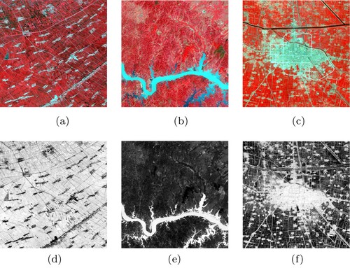
For Landsat images, the band-based SIs are important features expressing consistent information about a specific class. They can be used to compensate the uncertainty contained in CNN feature maps. In this study, three most commonly used SIs (as shown in Figure 1) are chosen as a case study to improve the generality of CNN on imperfect training samples. They are:

(1)	NDVI: defined by the difference between near-infrared band and red band, indicating the status of vegetation due to the high reflectivity of red band and high absorptivity of near-infrared band of plant canopy. It can be calculated as (4) $NDVI=\frac{NIR-Red}{NIR+Red}.$(4) NDVI highlights the existence of vegetation. As shown in Figure 1(a,d), the greater the NDVI value, the higher the vegetation density in the original Landsat image.
(2)	NDWI: defined by the difference between near-infrared band and green band (Mcfeeters 1996), indicating the status of water body since the green band is strongly absorbed and the near-infrared band is strongly reflected by water. Some other researchers also use mid-infrared band or short-wave near-infrared band (Gao 1996). The main difference between different definitions of NDWI lies in the information they expressed. Green band-based NDWI indicates the existence of water body itself, while mid-infrared- or short-wave near-infrared-based NDWI indicates the vegetation water content. In this study, the main purpose is to distinguish water body from other classes. Consequently, the following definition is employed: (5) $NDWI=\frac{Green-NIR}{Green+NIR}.$(5) Compared with CNN feature maps, NDWI is able to effectively highlight the features of water body, including small details (as shown in Figure 1 e).
(3)	NDBI (Normalized Difference Built-up index): indicates the density of built-up land. Its principle is similar to NDVI and NDWI. There are also two definitions about NDBI. One of them uses mid-infrared band and the other uses short-wave near-infrared band. In this study, the one used mid-infrared band is employed: (6) $NDBI=\frac{MIR-NIR}{MIR+NIR}.$(6)

Figure 1. Original images and corresponding remote sensing indices: (a) Vegetation; (b) Water body; (c) Built-up land; (d) NDVI; (e) NDWI; (f) NDBI.

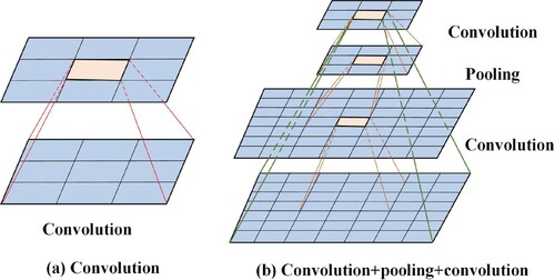
Fortunately, all the mentioned band-based SIs use larger values to represent features of the highlighted objects, which coincident with the pooling and activation functions of CNN. This consistency provides the possibility for the subsequent fusion of SIs and CNN feature maps. Concatenation is widely used for feature fusion in CNN. However, its fusion ability is limited by the receptive field (as shown in Figure 2 a). To overcome this drawback, a combination of convolution and pooling layers shown in Figure 2(b) is proposed to fully fuse the information contained in CNN feature maps and SIs. With a larger receptive field, the consistent information will be well fused with CNN feature maps, which is essential for classification. The two fusion strategies can be expressed as (7) $o=\sigma (w\times y_F+b)$(7) and (8) $o=\sigma (w_2\times pool(\sigma (w_1\times y_F+b_1))+b_2),$(8) where w is the parameter in the convolutional kernel, b is the corresponding bias, $pool\left(\cdot \right)$ is the maximum pooling, and $\sigma \left(\cdot \right)$ is the ReLU activation function.

Figure 2. Receptive field of one convolutional layer and two convolutional layers with an extra pooling layer.

3.4. Framework of TCNN-IN

Unlike CNN, which learns essential information from raw data, accurate SIs should be calculated from accurate surface reflectance product. To avoid surface reflectance product, a CNN branch is employed. Although CNN can approach the SIs as close as possible, the lack of constraints will lead to some learned values to exceed the range of $[-1,1]$. Therefore the nonlinear normalization in Equation (3(3) $y_{SI}=\{\begin{array}{ll}\frac{\log \left(x_{SI}\right)-min\{\log (x_{SI}\left)\right\}}{max\{\log (x_{SI}\left)\right\}-min\{\log (x_{SI}\left)\right\}}& \text{ x\_{SI} > 0}\\ 0& \text{ x\_{SI},=,0}\\ -\frac{\log (-x_{SI})-min\{\log (-x_{SI}\left)\right\}}{max\{\log (-x_{SI}\left)\right\}-min\{\log (-x_{SI}\left)\right\}}& \text{ x\_{SI} < 0.}\end{array}$(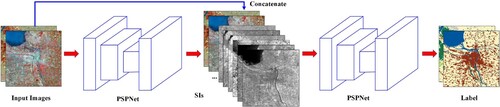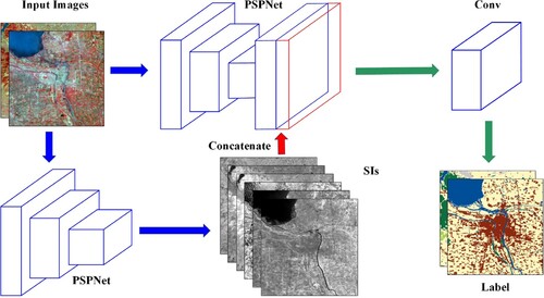3) ) is employed. In this section, four architectures are proposed to inject consistent information into CNN for improving generality and transferability. PSPNet is employed as the backbone due to its adaptability on multi-scale features, which are commonly appeared in Landsat images (Zhao et al. 2017). Archi1, shown in Figure 3, uses PSPNet to learn SIs and then concatenates them with the original images. The combination results are used as input of PSPNet for land cover mapping. Using x to represent the input image, the process can be expressed as (9) $o=CNN\left(cat\right(x,CN{N}_{SI}\left(x\right)\left)\right),$(9) where $CN{N}_{SI}\left(x\right)$ outputs the learned SIs.

Figure 3. Framework of Archi1 (batch_size=2).

The consistent information in SIs will be emerged by the following stacked convolutional layers, if SIs are concatenated with the original images. Archi2, which concatenate SIs with the CNN feature maps is proposed (as shown in Figure 4). This process can be expressed as (10) $o=cat\left(CN{N}_F\right(x),CN{N}_{SI}(x\left)\right),$(10) where $CN{N}_F\left(x\right)$ output feature maps learned from the original images. Then the output features are directly classified to achieve the final classification results.

Figure 4. The framework of Archi2 (batch_size=2).

Directly concatenating SIs and CNN feature maps is unexplainable, and the diversity of information is not well fused. Convolutional layer is a natural data fusion operation in both spatial and dimensional aspects. It is employed to further fuse SIs and CNN feature maps in Archi3 (shown in Figure 5). The corresponding calculation is expressed as (11) $o=conv\left(cat\right(CN{N}_F\left(x\right),CN{N}_{SI}\left(x\right)\left)\right).$(11)

Figure 5. The framework of Archi3 (batch_size=2).

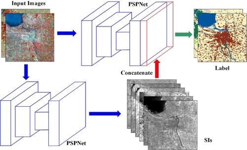
The fusion ability of convolutional layer is restricted by its size. To balance the trade-off between the number of parameters and the receptive field, a combination of $3\times 3$ convolutional layers and pooling layer is proposed to further fuse the learned features as shown in Figure 6. 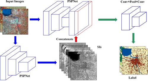The mathematical expression is (12) $o=conv\left(pool\right(conv\left(cat\right(CN{N}_F\left(x\right),CN{N}_{SI}\left(x\right)\left)\right)\left)\right).$(12) Archi4 concatenates SIs with the last layer of CNN feature maps and uses a combination of convolutional and pooling layers to further fuse them. In this way, the introduced consistent information will narrow the parameter space and improve the efficiency of network training. We believe that it can guide the network to learn general and transferable information from imbalanced training sets which contain noisy labels.

Figure 6. The framework of Archi4 (TCNN-IN) (batch_size=2).

3.5. Objective function

The overall objective of the proposed method consists of two components: the loss for the learned SIs and the loss for classification task. The loss for SIs evaluates the difference between estimated SIs and the corresponding ground truth. Accordingly, the mean square error can be used: (13) $Los{s}_{SI}=\frac{1}{N}\sum _{i=1}^N(o_{SI}-g_{SI}{)}^2,$(13) where $o_{SI}$ is the output of the CNN branch which estimates SIs, $g_{SI}$ is the corresponding ground truth, N is the total number of image pixels. Different from this branch, the loss for classification estimates the difference between the estimated distribution and the ground truth. Employing cross entropy as the loss function, the mathematical expression is (14) $Los{s}_{cla}=-\frac{1}{N}\sum _{i=1}^N\sum _{j=1}^c{g}_{cla}log\left(o_{cla}\right),$(14) where c is the number of classes, $g_{cla}$ is a one hot vector where the position of a single element 1 indicates its class, $o_{cla}$ is the output of CNN architecture which can be considered as the probability of estimated classes. The two objectives in Equations (13(13) $Los{s}_{SI}=\frac{1}{N}\sum _{i=1}^N(o_{SI}-g_{SI}{)}^2,$(13) ) and (14(14) $Los{s}_{cla}=-\frac{1}{N}\sum _{i=1}^N\sum _{j=1}^c{g}_{cla}log\left(o_{cla}\right),$(14) ) can be realized either separately or uniformly. Owing to the clear physical meaning of SIs, independently training CNN to estimate SIs or just use the digital value of Landsat image to produce SIs does not affect the stability of image features.

4. Experiments and discussion

4.1. Study area

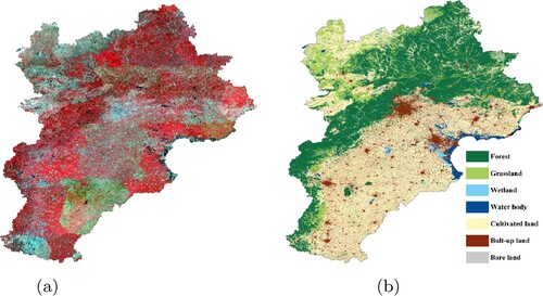
To test the proposed TCNN-IN (Archi4 shown in Figure 6), Jing-Jin-Ji region in the North of China is selected as the study area. The original Landsat image is shown in Figure 7(a). It is visually represented by near-infrared, red and green bands, in which the vegetation is red. All the six bands except the thermal infrared are used to train the network. Figure 7(a) is composed of Level 1T Landsat images of the year 2010 downloaded from https://earthexplorer.usgs.gov/ without any additional pre-processing. To train a CNN network, labels for the original images are necessary. Nevertheless, manually labeling for such a big area in pixel-wise is laborious. To avoid manually labeling, land-cover map with high overall accuracy is an alternative. Land Cover Map of the People's Republic of China (1:1000000) downloaded from http://www.geodata.cn/ has an overall accuracy of 94% for the first-level classes and 86% for the second-level classes throughout China. In this study, it is used as reference for the study area. To meet the resolution of Landsat images, the land cover map is rasterized to 30 m resolution. While, by comparing the reference with original Landsat images, we proposed to merge the second-level classes in the reference to seven first-level classes to fully utilize the expression ability of Landsat image, referencing the existing classification systems (Chen et al. 2015). The seven first-level classes are forest, grassland, wetland, water body, cultivated land, built-up land, and bare land. The merged first-level classification result is used as the reference as shown in Figure 7(b). Even so, class imbalance and noisy labels are still inevitable.

Figure 7. Original Landsat image and reference land-cover map: (a) Original Landsat image and (b) Reference.

4.2. The quality of training samples

1280 non-overlapping image patches with $512\times 512$ pixels are selected as training samples from Jing-Jin-Ji region. It has covered most of the study area. To avoid the impact of insufficient training samples on the network, 80% is used to construct the training set and the other 20% composes the validation set. This training set is called Training Set (TS)-1 in this paper. In the study area, labels of grassland and forest are highly confused due to their similar spectral features. Accordingly, these two classes are combined to construct TS-2 to explore the impact of sample quality. Considering the imbalanced distribution of classes, additional training samples about wetland are added to TS-1 to construct a new training set, called TS-3, because wetland occupies the least in the training samples. The additional samples are selected from Dongting Lake and Qiqihar Zhalong Wetland. To explore the effect of different proportions of inaccurate training samples, the areas containing forest and grassland are oversampled to increase the proportion of inaccurate training samples on the basis of TS-1 and TS-2, to construct TS-4 and TS-5. A description about the five training sets is listed in Table 1. The proportions of different classes in TS-1, TS-3, and TS-4 are shown in Figure 8 (TS-2 and TS-5 are not included since forest and grassland are combined).

Figure 8. Proportions of different classes in TS-1, TS-3, and TS-4.

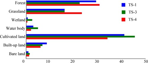
Table 1. Description of the training sets.

Name	Description
TS-1	Non-overlapping image patches from Jing-Jin-Ji region
TS-2	Merging forest and grassland in TS-1
TS-3	Adding wetland samples from Dongting Lake and Qiqihar Zhalong Wetland to TS-1
TS-4	Oversampling the forest and grassland area in TS-1
TS-5	Oversampling the forest and grassland area in TS-2

Using PSPNet as an example, the classification accuracies of the five training sets are shown in Table 2. Comparing classification accuracies of TS-1, TS-2 and TS-4, TS-5, it indicates that there did exist some confusion between the labels of forest and grassland. Combining these two classes can decrease the conflicting information contained in the training samples, and thus the corresponding classification accuracy is significantly improved. As shown in Figure 8, wetland occupies the least in TS-1. TS-3 increases the proportion of wetland, and increases the accuracy of wetland and overall accuracy by 26.11% and 0.93%, respectively. It can be concluded that adding additional information about minority classes cannot only increase the accuracy of the class, but also increase the overall accuracy. In TS-4, the areas mostly covered by grassland and forest are oversampled to increase the proportion of inaccurate training samples. By this way, the accuracy of grassland increases 18.56% and the overall accuracy increases 2.40%. TS-5 is obtained by oversampling the combined classes (forest and grassland). Although the classification of the merged class decreases, the overall accuracy increases about 0.1%. This indicates that, adding information about majority classes less impacted by noisy label can also improve the overall accuracy, but the improvement is not as obvious as adding minority class information (TS-3) or noisy label class information (TS-4). The experiment demonstrates the importance of additional information on the learning ability of CNN.

Table 2. Classification accuracy for the JingJinJi region of PSPNet on the five training sets, where forest and grassland are merged as one class in TS-2 and TS-5.

(%)	Forest	Grassland	Wetland	Water body	Cultivated land	Built-up land	Bare land	Overall accuracy
TS-1	81.54	36.05	41.82	71.66	90.34	47.50	37.73	75.25
TS-2	87.61		48.43	72.48	85.05	56.49	41.90	83.16
TS-3	85.18	49.41	67.93	72.40	83.97	56.10	43.86	76.18
TS-4	81.74	54.61	49.60	75.39	87.17	58.11	45.98	77.65
TS-5	85.64		53.68	73.04	85.91	65.39	50.74	83.26

4.3. Information entropy for image feature maps

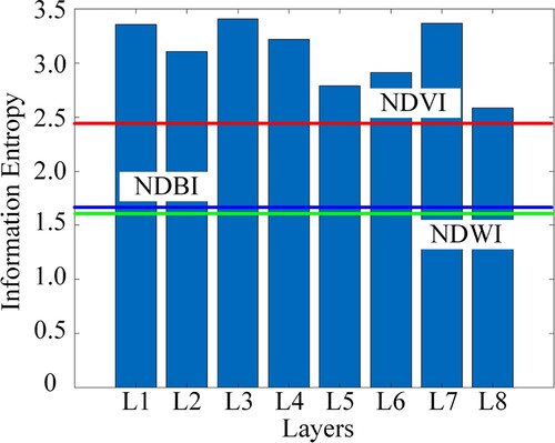
1280 training samples with $512\times 512$ pixels have covered most of the study area. To test the proposed CNN with imbalanced and noisy labels, half of the 1280 samples are selected as training samples and the other half construct the validation set. To evaluate the information contained in different feature maps, IEs of the first convolutional layer, the one after the pooling layer, four residual layers, pyramid pooling layer, and the classification layer of the original image (Figure 1a) are calculated and listed in Table 3 (the layers are represented by L1–L8 for convenience).

Table 3. Feature maps and corresponding entropy.

Table 2 visually exhibits the feature transformation process of CNN from lower layers to higher layers. IE decreases with the increase of CNN layers, except for the fourth residual layer (L6) and the pyramid pooling layer (L7). Before analyzing the reasons for the increase of IEs in L6 and L7, the difference of IEs between L1 and L2 are first discussed. L2 is the result of down sampling L1 to its half. This indicates that the size of feature maps has a significant impact on the IE. Feature maps with smaller size contain less information than those with larger size. Similarly, for the increasing of IE in L6 (the fourth residual layer), it is caused by the sudden increase of the number of convolutional kernels, which increases from 1024 to 2048. With the increasing of convolutional kernels, redundant information also increases, resulting in the increase of the IE in this layer. The same happens in the pyramid pooling layer. First, the feature maps are downsampled to different sizes, and then they are upsampled to the same size and concatenated. The concatenation of feature maps with different scales also introduces redundant information. That brings us to the problem of fusing CNN feature maps with SIs. Overall, the IEs of the feature maps decrease with the increasing of CNN layers and the information contained in higher-level layers is more likely to obtain satisfactory classification results. This indicates that the IE of higher-level feature maps is less than that in lower level feature maps and combine SIs with higher-level CNN feature maps is more efficient. That also gives an explanation for why minimizing loss functions of all the layers cannot improve the overall accuracy. This result is consistent with the assumption in Section 3.2.

The IEs of different CNN feature maps are expressed in histogram to visually compare them with the IEs of SIs. It is clear from Figure 9, all IEs of CNN feature maps are higher than the IEs of SIs. This indicates that features automatically learned by CNN is less consistent than SIs with clear physical meaning. But CNN features maps can be used for full class classification while SIs can only reflect some aspects of image features. To fully utilize the information complementarity, it is concluded that L8 is the most appropriate layer to combine with SIs.

Figure 9. IEs of CNN feature maps and SIs, where the red, green and blue lines represents the IEs of NDVI, NDWI and NDBI, respectively.

4.4. Experiments and analysis

The four architectures shown in Figure 3–6 are tested in this section. First, the employed SIs (NDVI, NDWI, and NDBI) are concatenated with the input images, corresponding network is called Archi1 for short. That is a commonly used method to take manually designed features into consideration in CNNs. As discussed in the last subsection, SIs have the closest IEs to that of the last layer of PSPNet. Therefore, it is believed that the stability of topological structure in these feature maps is equivalent in overall. Combining features with equivalent IEs may take fully use of information contained in these feature maps (Archi2). Moreover, concatenating features with equivalent IEs may encounter some problems caused by the inconsistency in numerical expression of features. For example, the value range of CNN feature maps is relative narrow due to the batch normalization layer, while most values distributed inside $[-1,1]$ for SIs employed in this study. To solve this problem, Archi3 which stacks a convolutional layer after concatenating and Archi4 which stacks a convolutional layer, a pooling layer and another convolutional layer, are proposed. Corresponding network structures are listed in Table 4. PSPNet is employed as a backbone to test the proposed architectures in this study.

Table 4. Names and structures of the networks used in this paper.

Name	Description
PSPNet	Backbone (Input images contains all the 6 bands of Landsat except the thermal infrared band)
Archi1	Combining SIs with the input images
Archi2	Combining SIs with the last layer
Archi3	Combining SIs with the last layer and using a convolutional layer to merge the information
Archi4	Combining SIs with the last layer and using a convolutional layer, a pooling layer, and another convolutional layer to merge the information

All the architectures are performed with pytorch in python and processed on a workstation with an Intel Xeon(R) Gold 5120 CPU(2.2 GHz), and four NVIDIA Tesla V100 GPU with 32GB memory. The batch size is set to 28, and the optimizer employed in this paper is Adam optimizer with an initial learning rate of ${10}^{-4}$ and a weight decay of ${10}^{-4}$. Corresponding classification results are shown in Figure 10. The original Landsat images are visually expressed in pseudo color composed of near-infrared, red and green bands. PSPNet can adjust to imperfect training samples to some extent, but the classification results tend to be over-fitted, especially on the classes heavily affected by noisy labels. The classification results shown in Figure 10(b3) is very close to its label (Figure 10(b2)), indicating large possibility of over fitting. In addition, it cannot recognize the wetland in Figure 10(a3) and misclassified the lower left corner in Figure 10(d3) as forest due to the imbalance and noisy labels in the training set. The consistent information in SIs are submerged when combined to the original images (Archi1). Consequently, the confusion among vegetation classes (grassland, forest and cultivated land) is obvious. As discussed in the last section, combining features with similar IEs can fully utilize the diversity of information. Therefore, the classification results are much better when SIs are combined with the last layer (Archi2). In addition, the number of bands in the last layer is much less than the former layers, which also provides an opportunity for SIs to play an important role.

Figure 10. Classification results of the networks, where (a1)–(d1) are original Landsat images; (a2)–(d2) are results in reference land-cover maps; (a3)–(d3) are classification results of PSPNet; (a4)–(d4) are classification results of Archi1; (a5)–(d5) are classification results of Archi2; (a6)–(d6) are classification results of Archi3, and (a7)–(d7) are classification results of Archi4.

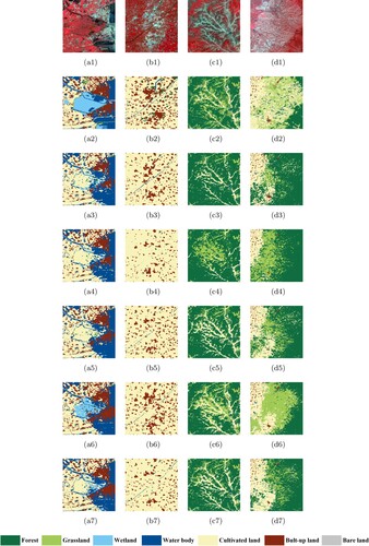
Considering the difference of the value range and corresponding data distribution between CNN feature maps and SIs, Archi3 and Archi4 shown in Figures 5 and 6 are proposed. Classification results of the two architectures are shown in Figure 10(a6) –(d6) and (a7) –(d7). Classification results of Archi3 are not as good as Archi2, indicating that insufficient fusion between CNN feature maps and SIs cannot fully utilize their diversity information. In contrast, enlarging the receptive field in Archi4 can better fuse the feature maps (as shown in Figure 10(a7) –(d7)). This experiment demonstrates that: (1) introducing consistent information can improve the learning ability of CNN; (2) both the selection of CNN layer and the fusion method are essential to force consistent information to contribute in the learning process of CNN; (3) proper feature fusion strategy constructs efficient capacity of the network and improves the learning ability of CNN.

The classification accuracies are listed in Table 5. The overall accuracies validate the discussion in the last section that combining feature maps with similar IEs is more efficient than combining image features with obvious different IEs. Comparing the overall accuracies of Archi3 and Archi4, it is clear that efficient feature fusion method also has a great impact on the learning ability of CNN. The classification accuracies of each class are positively correlated with the proportions of each class in the training set. As shown in Figure 11, cultivated land, forest, and grassland account for more than 85% in the training set. Accordingly, their classification accuracies have the most impact on the overall accuracy. In contrast, wetland and bare land account for the least in the training set and their impacts on the overall accuracy are limited. Archi4 achieves the highest overall accuracy not by the high classification accuracy of a certain class, but by the balanced recognition ability of all the classes.

Figure 11. Proportions of each class in the training set.

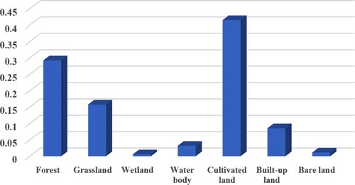
Table 5. Classification accuracies of the networks, where the bold indicates the best results.

	Forest	Grassland	Wetland	Water body	Cultivated land	Built-up land	Bare land	Overall accuracy
PSPNet	84.71	55.75	21.31	65.67	72.05	62.22	27.31	71.50
Archi1	82.55	40.66	21.27	65.59	80.04	56.22	26.78	71.88
Archi2	81.82	46.59	18.76	70.93	84.10	57.64	28.89	74.73
Archi3	77.44	61.08	23.70	67.52	81.11	61.85	34.85	74.58
Archi4	81.45	50.45	18.30	69.46	83.92	56.84	30.00	74.95

4.5. Experiments on the effects of different SIs

Different SIs reflect different aspects of image features. Affected by the stability of image features, the uncertainty degree (IE) of different SI is different. To further explore the impact of introducing image features with different degrees of uncertainty to CNN, single image index, two out of three, and all the three SIs are combined with CNN feature maps in this subsection. In this study, SIs are concatenated with the last layer of CNN network followed with a convolutional layer, a pooling layer and another convolutional layer (Archi4) due to its effectiveness demonstrated in the last section. Classification accuracies of networks with different SIs are listed in Table 6. From Table 6, the followings are concluded: (1) Combining CNN feature maps with SIs has a positive impact on the classification, indicating that introducing consistent information can improve the performance of CNN. (2) From the perspective of a single SI: combining with NDWI achieves the best performance among all three SIs. It indicates that the more consistent the introduced SI is, the better the classification results. This phenomenon can also be explained partially from the perspective of data distribution. As wetland occupies the least proportion in the training set, introducing more information about this class benefits the most among all the three SIs. (3) From the perspective of pairwise combination of SIs: the combination of NDWI and NDBI has the most obvious effect on the improvement of the learning ability of CNN, since these two SIs have the lowest IEs as shown in Figure 9. In contrast, the information contained in NDVI is as not consistent as NDWI and NDBI, and thus the accuracy improvement is not obvious when NDVI is involved. By comparing the class-wise accuracies and the overall accuracies, it can be found that the learning preference caused by unbalanced and noisy training samples can be improved when consistent information is injected, especially for minority classes. It can also be partially explained that, band-based SIs for minority classes is more consistent than automatically learned ones. Consequently, injecting consistent information makes CNN focus on detailed information instead of uncertainty or conflict information, and thus improves the learning ability of CNN. (4) The best performance is obtained when all three SIs are taken into account. The improvements not only lies in single or multi-classes, but in the balance among all the classes.

Table 6. Classification accuracies of networks with different spectral indices, where ‘–’ represents only the image bands are considered, and the others indicate the additional spectral indices. Bold indicates the best results.

	Forest	Grassland	Wetland	Water body	Cultivated land	Built-up land	Bare land	Overall accuracy
–	84.71	55.75	21.31	65.67	72.05	62.22	27.31	71.50
NDVI	79.62	58.18	25.03	73.27	78.50	58.29	34.32	73.35
NDWI	70.70	52.89	16.27	73.75	88.32	55.20	24.27	74.33
NDBI	78.41	54.67	16.44	60.86	80.69	56.04	26.10	72.95
NDVI+NDWI	67.14	35.36	17.16	66.09	89.50	64.30	36.06	72.12
NDVI+NDBI	90.02	37.36	19.85	64.10	74.49	63.93	35.93	71.57
NDWI+NDBI	84.06	48.19	25.55	72.64	80.82	64.99	34.99	74.76
ALL	81.45	50.45	18.30	69.46	83.92	56.84	30.00	74.95

Classification accuracies of classes corresponding to a certain remote sensing index are not clear in Table 6. Accuracies of different class types are listed in Tables 7–12. It can be seen from these tables that there is no obvious indication that the introduced consistent information about some classes has a direct impact on improving the classification accuracy of the corresponding classes. On the contrary, introducing consistent information contributes a lot on the improvement of overall accuracy. Actually, with the introduced consistent information, the network tries to learn more detailed information to achieve a global optimization. Thus, the uncertainty of CNN feature maps is greatly decreased. Therefore, the main role of the introduced consistent information which is represented in the form of SIs is to balance the learning preference of CNN, so as to decrease the uncertainty caused by imbalanced and noisy training samples. Benefited from the introduced consistent information, the problem of sacrificing detailed information and information about minority features is solved in some extent.

Table 7. Classification accuracies of networks including spectral indices about vegetation, where ‘–’ represents only the image bands are considered, and the others indicate the additional spectral indices. Underline highlights the classes under discussion, and bold indicates the best results.

	Vegetation	Wetland	Water body	Built-up land	Bare land	Overall accuracy
–	54.13	21.31	65.67	62.22	27.31	71.50
NDVI	51.45	25.03	73.27	58.29	34.32	73.35
NDVI+NDWI	43.60	17.16	66.09	64.30	36.06	72.12
NDVI+NDBI	57.24	19.85	64.10	63.93	35.93	71.57
ALL	52.36	18.30	69.46	56.84	30.00	74.95

Table 8. Classification accuracies of networks including spectral indices about water, where ‘–’ represents only the image bands are considered, and the others indicate the additional spectral indices. Underline highlights the classes under discussion, and bold indicates the best results.

	Forest	Grassland	Water	Cultivated land	Built-up land	Bare land	Overall accuracy
–	84.71	55.75	54.61	72.05	62.22	27.31	71.50
NDWI	70.70	52.89	51.66	88.32	55.20	24.27	74.33
NDVI+NDWI	67.14	35.36	34.76	89.50	64.30	36.06	72.12
NDWI+NDBI	84.06	48.19	47.44	80.82	64.99	34.99	74.76
ALL	81.45	50.45	52.36	83.92	56.84	30.00	74.95

Table 9. Classification accuracies of networks including spectral indices about Built-up land, where ‘–’ represents only the image bands are considered, and the others indicate the additional spectral indices. Underline highlights the classes under discussion, and bold indicates the best results.

	Forest	Grassland	Wetland	Water body	Cultivated land	Built-up land	Bare land	Overall accuracy
–	84.71	55.75	21.31	65.67	72.05	62.22	27.31	71.50
NDVI+NDBI	90.02	37.36	19.85	64.10	74.49	63.93	35.93	71.57
NDWI+NDBI	84.06	48.19	25.55	72.64	80.82	64.99	34.99	74.76
ALL	81.45	50.45	18.30	69.46	83.92	56.84	30.00	74.95

Table 10. Classification accuracies of networks including spectral indices about vegetation and water, where ‘–’ represents only the image bands are considered, and the others indicate the additional spectral indices. Underline highlights the classes under discussion, and bold indicates the best results.

	Vegetation+Water	Built-up land	Bare land	Overall accuracy
–	54.25	62.22	27.31	71.50
NDVI+NDWI	41.39	64.30	36.06	72.12
ALL	51.61	56.84	30.00	74.95

Table 11. Classification accuracies of networks including spectral indices about vegetation and built-up land, where ‘–’ represents only the image bands are considered, and the others indicate the additional spectral indices. Underline highlights the classes under discussion, and bold indicates the best results.

	Vegetation+Built-up land	Wetland	Water body	Bare land	Overall accuracy
–	63.23	21.31	65.67	27.31	71.50
NDVI+NDBI	66.00	19.85	64.10	35.93	71.57
ALL	68.38	18.30	69.46	30.00	74.95

Table 12. Classification accuracies of networks including spectral indices about water and built-up land, where ‘–’ represents only the image bands are considered, and the others indicate the additional spectral indices. Underline highlights the classes under discussion, and bold indicates the best results.

	Forest	Grassland	Water+Built-up land	Cultivated land	Bare land	Overall accuracy
–	84.71	55.75	67.79	72.05	27.31	71.50
NDWI+NDBI	84.06	48.19	72.65	80.82	34.99	74.76
ALL	81.45	50.45	75.47	83.92	30.00	74.95

4.6. Experiments on transferring ability

To test the transferability of the proposed TCNN-IN, four provinces around Jing-Jin-Ji region are selected as study areas, namely Shanxi, Henan, Shandong, and Liaoning. Inner Mongolia is not considered even it is adjacent to Jing-Jin-Ji region, due to its large geographical span. In this experiment, three time periods are taken into account including the same year of the trained model (2010). Original Landsat images of the four provinces in three time periods are shown in Figure 12. Shanxi locates in the west of Jing-Jin-Ji region. Most of this province is covered by forest and grassland, whose class distribution is obviously different from Jing-Jin-Ji region. Henan and Shandong are located in the south of Jing-Jin-Ji region. The surface coverage type of this region is similar to that of Jing-Jin-Ji region. Liaoning locates in the northeast of Jing-Jin-Ji region, and feature of the same surface coverage type is slightly different due to different vegetation types. From the perspective of different years, most of the original images in 2010 are collected from growing season, some of the original images covered 2005 are collected from non-growing season, while more images are from non-growing season in the year 2000.

Figure 12. Original Landsat images of the four provinces of three time-series.

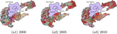
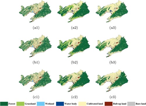
The models were trained using samples from the Jing-Jin-Ji region in2010 to predict the classification results for four provinces in China, for the years 2000, 2005, and 2010. The corresponding classification results are shown in Figures 13–16, for PSPNet and TCNN-IN (Archi4 in Table 4). In Figure 13, it is clear that the classification results of TCNN-IN are better than those of PSPNet for Shanxi Province. Although the vegetation classes are seriously affected by noisy labels, the improvements in recognizing these classes are obvious. This means that introducing consistent information can significantly improve the transferability of the CNN. As shown in Figure 14, both networks, regardless of the consistency of information, cannot accurately classify built-up land at the lower right corner of Henan Province. Considering the original Landsat images shown in Figure 12 and the referenced ground truth (Figure 14(a2)–(a3)), the inaccurate classifications are mainly caused by the distinctive spectral features of built-up land in this area. In contrast in Henan province, the transferred classification accuracy of built-up land in Shandong Province is obviously higher. The proposed TCNN-IN improved the ability of the CNN in recognizing built-up land during transfer, especially near the object boundaries. In addition, the classification of water body in the lower part is also improved when consistent information is taken into consideration. This enhancement is evident in 2005 and 2010, but not in 2000. A similar phenomenon can also be observed in Liaoning province, as shown in Figure 16. In these experiments, the transferred accuracies of vegetation type increased for most classes, NDVI performs the worst among all three SIs. These two conclusions can be explained by the fact that the main impact of introducing consistent information is to balance the learning ability of CNN on imbalanced and noisy labels, rather than to improve the classification accuracy of certain classes. Vegetation types contain noisiest labels among all classes, so the accuracies of these classes greatly improve when consistent information is introduced.

Figure 13. Transferred classification results of Shanxi Province; where (a), (b), (c) represents the years of 2000, 2005 and 2010, and (1), (2), (3) represents the ground truth, PSPNet, and TCNN-IN.

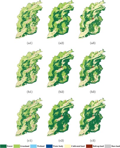
Figure 14. Transferred classification results of Henan Province; where (a), (b), (c) represent the years of 2000, 2005 and 2010, and (1), (2), (3) represent the ground truth, PSPNet, and TCNN-IN.

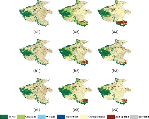
Figure 15. Transferred classification results of Shandong Province; where (a), (b), (c) represent the years of 2000, 2005, and 2010, and (1), (2), (3) represent the ground truth, PSPNet, and TCNN-IN.

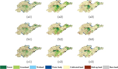
Figure 16. Transferred classification results of Liaoning Province; where (a), (b), (c) represent the years of 2000, 2005, and 2010, and (1), (2), (3) represent the ground truth, PSPNet, and TCNN-IN.

The overall classification accuracies for the four provinces during the three time periods are listed in Table 13. To further explore the correlation between the transferability of CNN and data distribution, the proportions of different classes in the training samples for Shanxi, Henan, Shandong and Liaoning provinces are listed in Figure 17. In Table 13, it is observed that the overall accuracies are the worst for the Shanxi Province among the four areas studied. In contrast, the transferred classification of Shandong is the best among all four provinces. Comparing the distributions with the training samples of Jing-Jin-Ji region in Figure 17, it is more similar of the distributions between Shandong Province and the Jing-Jin-Ji region than the distributions between Shanxi Province and the Jing-Jin-Ji region. The distribution for the Liaoning Province is most similar to that of the training samples. However, the difference in climate leads to different features of the same class, in particular the vegetation type may vary according to species since it is located in the northeast of Jing-Jin-Ji region. Although the features of the classes for Liaoning Province are different from those of the training samples, TCNN-IN displays better transferability and higher overall accuracy in this region compared with PSPNet. This means that the proposed TCNN-IN can clearly improve the learning and transferring ability of the CNN. The improvement in transferability is restricted by the similarity between the source dataset and target images. The more similar the features, the more accurate the classification results are. From the perspective of geographical distribution, trained models with consistent information perform well in adjacent regions with similar class distributions and spectral features.

Figure 17. Proportions of different classes in the training samples (Jing-Jin-Ji region), Shanxi, Henan, Shandong, and Liaoning provinces.

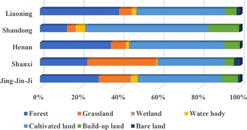
Table 13. Classification accuracies of the four provinces in the three time periods.

Year	(%)	Shanxi	Henan	Shandong	Liaoning
2000	PSPNet	67.25	67.40	74.37	67.78
	TCNN-IN	68.49	72.52	77.68	73.18
2005	PSPNet	54.90	66.70	67.06	63.73
	TCNN-IN	65.73	71.99	72.48	71.25
2010	PSPNet	63.16	65.06	66.52	59.24
	TCNN-IN	63.56	68.46	72.42	69.15

5. Conclusion

This paper proposes injecting certainty information into CNN to improve the learning ability under imbalanced and noisy labels. To reflect the stability of the image features, three commonly used band-based SIs were selected to provide consistent information. To determine the appropriate layer to inject consistent information into, IE was introduced to estimate the uncertainty of the CNN feature maps and SIs. From the experiments, it can be concluded that the more consistent the injected information, the more the learning ability of the CNN is improved. The role of the injected consistent information is not only to improve the recognition ability of certain classes but also to balance the learning ability of all classes under imbalanced and noisy labels. Thus, both generality and transferability were significantly improved in the proposed TCNN-IN. The overall accuracy was improved about 3.45% and the accuracy of transferability was increased by 10.83% at most. The proposed TCNN-IN provides a new option for time-series and cross-regional land-cover mapping, which is urgently needed in agriculture, ecosystems, and corresponding research.

Improving the learning ability of CNN networks through consistent information is challenging. This study employed three commonly used band-based SIs to provide consistent information, as a preliminary test. Further work is planned on manually designing different types of features and exploring their complementarity with CNN feature maps. Further, the focus is expected to be on the feature learning process of deep CNN models to explore the dynamic changes in the degree of uncertainty in CNN feature maps as well as the learning process itself. In addition, a more accurate method for introducing consistent information into CNN feature maps is also of interest.

Data availability statement

The data that support the findings of this study are openly available in USGS at https://earthexplorer.usgs.gov/ and in the National Earth System Science Data Center at http://www.geodata.cn/.

Disclosure statement

No potential conflict of interest was reported by the author(s).

Additional information

Funding

This work was supported by National Natural Science Foundation of China [41801233, 41761087] Ningbo Science and Technology Innovation Project [2020Z019] Natural Science Foundation of Guangxi Province [2020GXNSFBA159012].

References

- Akar, O., and O. Gungor. 2015. “Integrating Multiple Texture Methods and NDVI to the Random Forest Classification Algorithm to Detect Tea and Hazelnut Plantation Areas in Northeast Turkey.” International Journal of Remote Sensing 36 (2): 442–464.
- Akilan, T., Q. M. Jonathan Wu, A. Safaei, and Wei Jiang. 2017. “A Late Fusion Approach for Harnessing Multi-CNN Model High-Level Features.” In 2017 IEEE International Conference on Systems, Man, and Cybernetics (SMC), 566–571.
- Aslam, Arsalan, Muhammad Navved Salik, Faisal Chughtai, Nouman Ali, Hanif Dar, and Saadat Tehmina Khalil. 2019. “Image Classification Based on Mid-Level Feature Fusion.” In 2019 15th International Conference on Emerging Technologies (ICET), 1–6. IEEE.
- Bria, Alessandro, Claudio Marrocco, and Francesco Tortorella. 2020. “Addressing Class Imbalance in Deep Learning for Small Lesion Detection on Medical Images.” Computers in Biology and Medicine120: 103735.
- Chen, Jun, Jin Chen, Anping Liao, Xin Cao, Lijun Chen, Xuehong Chen, Chaoying He, et al. 2015. “Global Land Cover Mapping At 30 m Resolution: A POK-Based Operational Approach.” ISPRS Journal of Photogrammetry and Remote Sensing 103: 7–27. Global Land Cover Mapping and Monitoring.
- Chen, S., C. Tao, X. Wang, and S. Xiao. 2018. “Polsar Target Classification Using Polarimetric-Feature-Driven Deep Convolutional Neural Network.” In IGARSS 2018 – 2018 IEEE International Geoscience and Remote Sensing Symposium, 4407–4410.
- Chun, H., M. Kim, J. Kim, K. Kim, J. Yu, T. Kim, and S. Han. 2019. “Adaptive Exploration Harmony Search for Effective Parameter Estimation in An Electrochemical Lithium-Ion Battery Model.” IEEE Access 7: 131501–131511.
- Feng, Wei, Yinghui Quan, Gabriel Dauphin, Qiang Li, Lianru Gao, Wenjiang Huang, Junshi Xia, Wentao Zhu, and Mengdao Xing. 2021. “Semi-Supervised Rotation Forest Based on Ensemble Margin Theory for the Classification of Hyperspectral Image with Limited Training Data.” Information Sciences 575: 611–638.
- Gadzicki, Konrad, Razieh Khamsehashari, and Christoph Zetzsche. 2020. “Early vs Late Fusion in Multimodal Convolutional Neural Networks.” In 2020 IEEE 23rd International Conference on Information Fusion (FUSION), 1–6.
- Gangappa, M., K. Mai, and C. P. Sammulal. 2018. “An NDVI Based Spatial Pattern Analysis for Spatial Image Classification.” International Journal of Applied Engineering Research 13 (14): 11553–11558.
- Gao, Bocai. 1996. “NDWI A Normalized Difference Water Index for Remote Sensing of Vegetation Liquid Water From Space.” Remote Sensing of Environment 58 (3): 257–266.
- Ghaseminik, Fariba, Hossein Aghamohammadi, and Mohsen Azadbakht. 2021. “Land Cover Mapping of Urban Environments Using Multispectral LiDAR Data Under Data Imbalance.” Remote Sensing Applications: Society and Environment 21: 100449.
- Goodfellow, I., Y. Bengio, and A. Courville. 2016. Deep Learning.
- Jia, Dongyao, Zhengyi Li, and Chuanwang Zhang. 2020. “Detection of Cervical Cancer Cells Based on Strong Feature CNN-SVM Network.” Neurocomputing 411: 112–127.
- Jia, Kun, Shunlin Liang, Xiangqin Wei, Yunjun Yao, Yingru Su, Bo Jiang, and Xiaoxia Wang. 2014. “Land Cover Classification of Landsat Data with Phenological Features Extracted From Time Series MODIS NDVI Data.” Remote Sensing 6 (11): 11518–11532.
- Kansakar, P., and A. Munir. 2018. “A Design Space Exploration Methodology for Parameter Optimization in Multicore Processors.” IEEE Transactions on Parallel and Distributed Systems 29 (1): 2–15.
- Krawczyk, Bartosz. 2016. “Learning from Imbalanced Data: Open Challenges and Future Directions.” Progress in Artificial Intelligence 5 (4): 221–232.
- LeCun, Yann, Yoshua Bengio, and A Courville. 2016. Deep Learning. The MIT Press.
- Li, Ou, and Peng-lang Shui. 2020. “Subpixel Blob Localization and Shape Estimation by Gradient Search in Parameter Space of Anisotropic Gaussian Kernels.” Signal Processing 171: 107495.
- Liang, C., H. Zhang, D. Yuan, and M. Zhang. 2020. “A Novel CNN Training Framework: Loss Transferring.” IEEE Transactions on Circuits and Systems for Video Technology 30 (12): 4611–4625.
- Liu, P., J. Guo, C. Wu, and D. Cai. 2017. “Fusion of Deep Learning and Compressed Domain Features for Content-Based Image Retrieval.” IEEE Transactions on Image Processing 26 (12): 5706–5717.
- Liu, Qinghui, Michael Kampffmeyer, Robert Jenssen, and Arnt-Brre Salberg. 2020. “Dense Dilated Convolutions Merging Network for Land Cover Classification.” IEEE Transactions on Geoscience and Remote Sensing 58 (9): 6309–6320.
- Lv, Qinzhe, Wei Feng, Yinghui Quan, Gabriel Dauphin, Lianru Gao, and Mengdao Xing. 2021. “Enhanced-Random-Feature-Subspace-Based Ensemble CNN for the Imbalanced Hyperspectral Image Classification.” IEEE Journal of Selected Topics in Applied Earth Observations and Remote Sensing14: 3988–3999.
- Mcfeeters, KS. 1996. “The Use of the Normalized Difference Water Index (NDWI) in The Delineation of Open Water Features.” International Journal of Remote Sensing 17: 1425–1432.
- Nalepa, Jakub, Michal Myller, and Michal Kawulok. 2020. “Training- and Test-Time Data Augmentation for Hyperspectral Image Segmentation.” IEEE Geoscience and Remote Sensing Letters 17 (2): 292–296.
- Nalepa, Jakub, Michal Myller, and Michal Kawulok. 2020. “Transfer Learning for Segmenting Dimensionally Reduced Hyperspectral Images.” IEEE Geoscience and Remote Sensing Letters 17 (7): 1228–1232.
- Pezzano, Giuseppe, Vicent Ribas Ripoll, and Petia Radeva. 2021. “CoLe-CNN: Context-learning Convolutional Neural Network with Adaptive Loss Function for Lung Nodule Segmentation.” Computer Methods and Programs in Biomedicine 198: 105792.
- Ramanath, Anushree, Saipreethi Muthusrinivasan, Yiqun Xie, Shashi Shekhar, and Bharathkumar Ramachandra. 2019. “NDVI Versus CNN Features in Deep Learning for Land Cover Classification of Aerial Images.” In IGARSS 2019-2019 IEEE International Geoscience and Remote Sensing Symposium, 6483–6486. IEEE.
- Sasidhar, T. T., K. Sreelakshmi, M. T. Vyshnav, S. Vishvanathan, and K. P. Soman. 2019. “Land Cover Satellite Image Classification Using NDVI and SimpleCNN.” In 2019 10th International Conference on Computing, Communication and Networking Technologies (ICCCNT), 1–5.
- Shannon, C. E. 1948. “A Mathematical Theory of Communication.” The Bell System Technical Journal27 (4): 623–656.
- Shao, Yang, Ross S. Lunetta, Brandon Wheeler, John S. Iiames, and James B. Campbell. 2016. “An Evaluation of Time-Series Smoothing Algorithms for Land-Cover Classifications Using MODIS-NDVI Multi-Temporal Data.” Remote Sensing of Environment 174: 258–265.
- Szabo, Szilard, Zoltan Gacsi, and Boglarka Balazs. 2016. “Specific Features of NDVI, NDWI and MNDWI As Reflected in Land Cover Categories.” Lethaia 10: 194–202.
- Taherkhani, Aboozar, Georgina Cosma, and T. M. McGinnity. 2020. “AdaBoost-CNN: An Adaptive Boosting Algorithm for Convolutional Neural Networks to Classify Multi-Class Imbalanced Datasets Using Transfer Learning.” Neurocomputing 404: 351–366.
- Taufik, Afirah, Sharifah Sakinah Syed Ahmad, and Nor Fatin Emiliza Khairuddin. 2017. “Classification of Landsat 8 Satellite Data Using Fuzzy c-means.” In International Conference on Machine Learning & Soft Computing, 58–62.
- Wang, Y., T. Peng, J. Duan, C. Zhu, J. Liu, J. Ye, and M. Jin. 2020. “Pathological Image Classification Based on Hard Example Guided CNN.” IEEE Access 8: 114249–114258.
- Wei, Y., C. Gong, S. Chen, T. Liu, J. Yang, and D. Tao. 2020. “Harnessing Side Information for Classification Under Label Noise.” IEEE Transactions on Neural Networks and Learning Systems 31 (9): 3178–3192.
- Zhang, Ce, Paula A. Harrison, Xin Pan, Huapeng Li, Isabel Sargent, and Peter M. Atkinson. 2020. “Scale Sequence Joint Deep Learning (SS-JDL) for Land Use and Land Cover Classification.” Remote Sensing of Environment 237: 111593.
- Zhang, Qian, Feifei Lee, Ya Gang Wang, Ran Miao, Lei Chen, and Qiu Chen. 2020. “An Improved Noise Loss Correction Algorithm for Learning From Noisy Labels.” Journal of Visual Communication and Image Representation 72: 102930.
- Zhao, Hengshuang, Jianping Shi, Xiaojuan Qi, Xiaogang Wang, and Jiaya Jia. July, 2017. “Pyramid Scene Parsing Network.” In Proceedings of the IEEE Conference on Computer Vision and Pattern Recognition (CVPR).
- Zhao, Bo, Xianmin Zhang, Hai Li, and Zhuobo Yang. 2020. “Intelligent Fault Diagnosis of Rolling Bearings Based on Normalized CNN Considering Data Imbalance and Variable Working Conditions.” Knowledge-Based Systems 199: 105971.
- Zhou, Tianyu, Zhenjiang Miao, and Jianhu Zhang. 2018. “Combining CNN with Hand-Crafted Features for Image Classification.” In 2018 14th IEEE International Conference on Signal Processing (ICSP), 554–557. IEEE.