A method for reconstructing NDVI time-series based on envelope detection and the Savitzky-Golay filter

ABSTRACT

High-quality, normalized differential vegetation index (NDVI) time-series data are fundamental for environmental remote sensing applications; however, their quality is often influenced by complicated factors such as atmospheric aerosols and cloud coverage. Hence, in the current study, a robust reconstruction method based on envelope detection and the Savitzky-Golay filter (ED-SG) was developed to reduce noise in the NDVI time-series. To verify the performance of ED-SG, simulation experiments were implemented and NDVI time-series samples were selected for different land cover types derived from MOD09GQ, Sentinel-2 and Landsat 8 OLI of Yangtze River Basin, between December 2018 and December 2019. The experimental results yielded an agreement coefficient and variance of 0.9599 and 0.0006, respectively on simulated time-series, Additionally, the smoothness metrics of evergreen broadleaf forests, evergreen needleleaf forests, deciduous broadleaf forests, herbaceous, and croplands were 0.0019, 0.0017, 0.0012, 0.0012, and 0.0013, respectively. Ultimately, the reconstructed time-series metrics showed significant improvements in robustness and smoothness over conventional methods. Moreover, the simplistic mechanisms of the ED-SG model enabled it to run effectively in the Google Earth Engine over the NDVI time-series of the whole Yangtze River Basin.

KEYWORDS:

• Time-series reconstruction
• envelope detection
• Savitzky-Golay filter
• Google Earth Engine

1. Introduction

Remote sensing vegetation indexes such as the normalized differential vegetation index (NDVI) are commonly used to enhance vegetation characteristics in remote sensing images. NDVI time-series have been proven effective in reflecting the phenology of vegetation, which are widely used in remote sensing applications, including identifying vegetation activity (de Jong et al. 2011; Li et al. 2019), phenology extraction (Vrieling, de Beurs, and Brown 2011; Hmimina et al. 2013; Li et al. 2017), land cover classification (Geerken, Zaitchik, and Evans 2005; Jin et al. 2018; Sun, Fagherazzi, and Liu 2018; Liu et al. 2020), drought monitoring (Ji and Peters 2003; Gu et al. 2007), and so on. However, NDVI time-series are susceptible to different types of noise based on the precision and calibration of the sensors, atmospheric attenuation, and off-nadir viewing, among other factors, all of which may lead to deviations in NDVI calculations (Goward et al. 1991; Hird and McDermid 2009). In particular, low-value noise commonly caused by clouds and shadows are major challenges faced by reconstruction methods (Gong et al. 2006). Although some sensors (e.g. Moderate Resolution Imaging Spectroradiometer (MODIS)) with high calibration accuracy have increased data quality by correcting for the influence of gaseous absorption, atmospheric aerosol scattering, coupling between the atmospheric and surface bidirectional reflectance function (BRDF), and the adjacency effect (atmospheric point spread function) (Vermote, El Saleous, and Justice 2002), the residual influences persist in the NDVI time-series (Huete and Liu 1994; Gao et al. 2002). These influences may interfere with the accuracy of subsequent applications. Accordingly, it is imperative to pre-process the NDVI time-series through a reliable reconstruction method to minimize the influences of noise.

Presently, numerous reconstruction methods based on different assumptions have been employed in a variety of application scenarios (Hird and McDermid 2009; Julien and Sobrino 2010; Kandasamy et al. 2013). Linear interpolation (LI) (Zhao et al. 2009) and maximum value composite (MVC) (Holben 1986) are the earlier classical time-series reconstruction methods. However, LI simply replaces the noise with linear estimation without considering vegetation growth, while MVC ignores many details of the time-series. These methods can only reduce major perturbations, and additional filtering is typically required to obtain smooth NDVI profiles (Atzberger and Eilers 2011a). An alternative strategy involves fitting the original data by asymmetric function (commonly, asymmetric Gaussian (Jonsson and Eklundh 2002) and double logistic (Jönsson and Eklundh 2004) functions). While these methods effectively improved the quality of single-season NDVI time-series, they cannot be applied to those with multi- or no seasonal features. In fact, some filtering methods can be adapted to NDVI time-series with multi-seasonal features and can be divided into local filtering methods (e.g. Savitzky-Golay filter (Savitzky and Golay 1964)), and overall filtering methods (e.g. harmonic analysis, HANTS (Cihlar 1996; Yang et al. 2015; Zhou, Jia, and Menenti 2015), and Whittaker smoother, WS (Whittaker 1923; Kong et al. 2019)); however, these methods cannot distinguish noise from original data and particularly underestimate NDVI in the reconstructed time-series, especially with higher temporal resolution and denser-noise time-series. Mean-value iteration filter (MVI) (Ma and Veroustraete 2006), the Best Index Slope Extraction (BISE) (Viovy, Arino, and Belward 1992), and its improved method (Lovell and Graetz 2001) were developed to extract the upper envelope of the NDVI time-series, and have proven effective at eliminating the influence of low-value noise caused by clouds and shadows. However, their capability of dealing with other types of noise, such as those caused by atmospheric variability and bidirectional effects, as well as the smoothness of the reconstructed time-series, may be insufficient.

Due to the limitations associated with a single method, it is not uncommon to combine different reconstruction methods to conducted multi-step time-series reconstruction. For instance, Chen et al. used LI to replace the cloudy NDVI values and, subsequently, used SG filter to obtain smooth time-series (Chen et al. 2004). Carvalho Junior et al. then further proposed a method to use SG filter to detect outlier NDVI values and conducted LI and SG filter to reconstruct NDVI time-series (de Carvalho Júnior et al. 2015). More recently, the development of the Google Earth Engine (GEE) has provided an opportunity to enlarge the spatiotemporal scale of remote sensing research (Chen et al. 2017; Gorelick et al. 2017; Teluguntla et al. 2018; Parente et al. 2019; Gumma et al. 2020); however, few applicable denoising algorithms for GEE exist owing to its unique operation mode (Kong et al. 2019). For example, to guarantee the computing efficiency, GEE does not permit time-series computing pixel by pixel; moreover, the way by which GEE traverses images differs from that of other platforms, making the reconstruction methods, such as MVI and BISE, difficult to conduct. Besides, asymmetric Gaussian and double logistic analysis are only applicable for vegetation with a clear seasonal pattern, which is difficult to automatically obtain by GEE. Thus, to overcome the limitations of conventional methods, it is necessary to develop an NDVI time-series reconstruction method that is sufficiently robust to handle various noise conditions and is compatible with GEE.

To this end, in the current study, an NDVI time-series reconstruction method based on envelope detection and the Savitzky-Golay filter (ED-SG) is proposed. To assess the accuracy of this method, ED-SG was first compared to conventional algorithms (SG, HANTS, WS, MVI, and BISE) using simulated NDVI time-series and those derived from multi-sensor remote sensing NDVI time-series. The daily NDVI time-series (MOD09GQ-NDVI) was computed by the MOD09GQ product derived from MODIS surface reflectance data to verify the performance of the reconstructions with high temporal resolution NDVI time-series. Subsequently, the flexibility of the method on different spatial-temporal resolution NDVI time-series from Sentinel-2 MIS (Sentinel-NDVI) and Landsat 8 OLI (Landsat-NDVI) was analyzed. Of note, to assess the accuracy, the comparison between ED-SG and conventional algorithms was based on the one-pixel NDVI time-series; the conventional algorithms, such as MVI and BISE, may not achieve satisfactory efficiency on the GEE platform. Therefore, these experiments were conducted on an offline Python-Anaconda environment. To ensure the ability to evaluate the ED-SG on GEE, the study area was the Yangtze River Basin, one of China’s most important agricultural areas, whose unique ecological environment is valuable for comparative research. Moreover, the complicated vegetation distribution, terrain, meteorological conditions and large spatial scale of the study area can provide sufficient ideal samples for the evaluation of the experimental methods. Finally, to assess the potential of ED-SG with the GEE platform, the method was programmed to be conducted on GEE, and its reliability was discussed via analyses of the relationship between the original NDVI time-series, the reconstructed NDVI time-series, and gross primary production (GPP).

2. Materials and methods

2.1. Study area and data

The study area was the Yangtze River Basin, covering 1.8 million km² of eastern, central, and southwestern China. It is an area of plentiful, although spatially imbalanced, water resources (Wei, Chang, and Dai 2014) owing to the influence of climate, dynamic water vapor, terrain, and other regional factors (Xu et al. 2008). Temperature increases from northeast to southwest, and the 0°C accumulated temperature boundary is in the plateau area of south Qinghai, west Sichuan, and the valleys of the Hengduan Mountains. The average annual temperature of the study area is 12.6–28.3°C, and the average annual precipitation is 500–2500 mm (Qu et al. 2020).

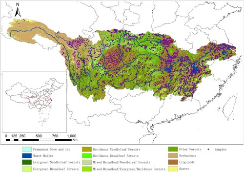
Figure 1 illustrates the land cover of the Yangtze River Basin according to the MODIS MCD12Q1 Land Cover Type image of 2019. MCD12Q1 supplies 500 m global maps of land cover at annual time steps (Sulla-Menashe and Friedl 2018). The product is open access from Land Processes DAAC or GEE. The study area is dominated by evergreen needleleaf and broadleaf forests, deciduous broadleaf forests, and herbaceous plants. In addition, croplands are abundant in the middle and lower reaches (shown in Figure 1 by 30 m Global Food Security-support Analysis Data, GFSAD30, cropland distribution product (Oliphant et al. 2017)). Samples were randomly selected from the study area for all subsequent experiments. For cropland samples, only those MCD12Q1 pixels fully covered by GFSAD30 ‘croplands’ pixels were regarded as effective samples. It should be noted that the vegetation types within the study area are complex, and many croplands are interplanted, all creating mixed pixels in the imagery, especially for 500 m moderate resolution products like MCD12Q1 (Ma et al. 2015; Yang et al. 2017). Accordingly, the selected samples were filtered to minimize the influence of mixed pixels. According to the quality control (QC) and quality assurance (QA) flags of MCD12Q1 data, only those pixels with a confidence >80% were regarded as qualified samples. Landsat-8 OLI images (spatial resolution, 30 m) were also referenced when selecting pure pixel sample sites.

Figure 1. Landcover of the Yangtze River Basin and sample site distribution. The land cover map is derived from the MCD12Q1 (Friedl and Sulla-Menashe 2015) image and GFSAD30 (Teluguntla et al. 2017) image.

Multi-sensor data including MODIS, Landsat 8 OLI, and Sentinel-2 MIS images were collected from December 2018 to December 2019 (Table 1), and all images were obtained through GEE. The images ingested into GEE are pre-processed to facilitate fast and efficient access, and the surface reflectance products we used here have been atmospherically corrected (Gorelick et al. 2017). Other indispensable preprocessing includes temporal and location filtering and NDVI time-series computing to generate the NDVI time-series.

Table 1. Remote sensing imagery data employed in the analysis.

Product	Spatial Resolution	Temporal Resolution	Purpose	Source
GFSAD30	30 m	–	Croplands distribution	https://www.usgs.gov/centers/wgsc/science/global-food-security-support-analysis-data-30-m-gfsad?qt-science_center_objects=0#qt-science_center_objects
MCD12Q1	500 m	–	Sample selection	https://lpdaac.usgs.gov/products/mcd12q1v006/
MOD09GQ	250 m	1 day	Generate MOD09GQ-NDVI	https://lpdaac.usgs.gov/products/mod09gqv006/
MOD09GA	500 m	1 day	Obtain QC & QA flags	https://lpdaac.usgs.gov/products/mod09gav006/
Sentinel-2 MIS, Level-2A	10 m	5 days	Generate Sentinel-NDVI	https://sentinels.copernicus.eu/web/sentinel/user-guides/sentinel-2-msi
Landsat 8 Surface Reflectance, Tier 1	30 m	16 days	Generate Landsat-NDVI	https://www.usgs.gov/core-science-systems/nli/landsat/landsat-collection-1-surface-reflectance
MOD17A2H	500 m	–	NDVI-GPP relativity test	https://lpdaac.usgs.gov/products/mod17a2hv006/

2.2. Envelope detection and Savitzky-Golay filter

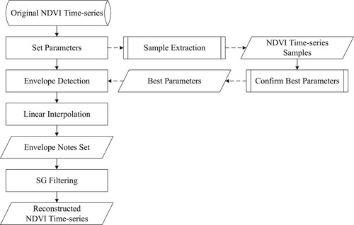
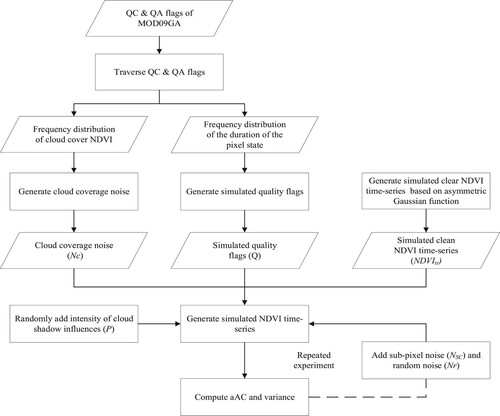
The principle of the ED-SG method is based on the following three assumptions: (1) vegetation growth is stable, resulting in a smooth NDVI time-series; (2) clouds and poor atmospheric conditions typically suppress NDVI values; and (3) all other sources of noise are categorized as random noise. ED is used to eliminate low-value noise by searching for the envelope nodes of the time-series, which are then smoothed by the SG filter to minimize the influence of random noise. The workflow of ED-SG is briefly shown in Figure 2.

Figure 2. Conceptual scheme of the proposed ED-SG method.

2.2.1. Envelope detection

ED is a type of high-pass filtering based on a discriminant function that eliminates low-value noise while retaining high-value NDVI as envelope nodes. Compared to conventional envelope extraction methods, such as BISE, ED requires fewer parameters and has a simpler distinguish condition, which makes the method suitable for cloud platforms such as GEE to conduct envelope extraction on the whole NDVI time-series image collection. Given an original NDVI time-series $O$, envelope nodes $E$, and last envelope node $e_i$, setting the first NDVI value of $O$ ($o_0$) as the start of $E$ ($e_0$), and then chronologically traversing $O$, the discriminant function of time $t$ can be expressed according to Eq. (1): (1) $f\left(t\right)={\left({\displaystyle \frac{\sigma }{1+\sigma }}\right)}^{t-i}{e}_i$(1) where $\sigma$ is the attenuation parameter used to control the rate of decline in the discriminant function. A smaller $\sigma$ causes the discriminant function to decline rapidly and identifies low NDVI points as envelope nodes. In contrast, if $\sigma$ is large, the discriminant function will decline slower, which tends to exclude low NDVI values (the precise effect of the $\sigma$ on the reconstruction result will be discussed in Section 3.1). When calculating the algorithm, if the original NDVI of time $t$ ($o_t$) satisfies Eq. (2): (2) $o_t-f\left(t\right)\ge 0$(2) where $o_t$ is inserted as the new $e_i$. After traversing $O$, the envelope nodes are linearly interpolated, creating the original envelope node set of the NDVI time-series, $E^{\mathrm{\prime }}$.

2.2.2. Savitzky-Golay filter

After envelope detection, the random noise, presented within the envelope nodes set prevents the assumption that the NDVI time-series are smooth from being met; thus, an SG filter to further smoothen the envelope was used. Savitzky and Golay (1964) proposed a simplified least-squares fit convolution for smoothing and computing derivatives of a set of consecutive values (Savitzky and Golay 1964). This method can be considered as a weighted moving average filter, with the weight given by a polynomial of a certain degree (Chen et al. 2004) and is calculated according to Eq. (3): (3) $r_t={\displaystyle \frac{1}{n}\sum _{j=-m}^{j=m}{c}_j{e}_{t+j}^{{}^{\mathrm{\prime }}}}$(3) where $e_t^{\mathrm{\prime }}$ is the NDVI of time $t$ in envelope nodes $E^{\mathrm{\prime }}$, $r_t$ is the NDVI smoothed by the SG filter, $j$ is the distance from $t$, $c_j$ is the weighting coefficient, $n$ is the size of the moving smooth window (equal to 2m+1), and $m$ is the half-width size of the smooth window. Values of m < 2 months can be considered as appropriate parameters for generating the long-term change trend curve (Chen et al. 2004). For MOD09GQ-NDVI, $m$ was set as 15, and a third-degree polynomial was used to set the weighting coefficient.

2.3. Evaluating ED-SG performance

Considering that no field measurement dataset exists over such a large spatiotemporal scale, it was impracticable to directly validate the reconstructed NDVI time-series quality (Liu et al. 2020). In practice, indirect or qualitative methods are commonly used to this end (Hird and McDermid 2009; Julien and Sobrino 2010; Atzberger and Eilers 2011b), and here, simulation and qualitative evaluation experiments were designed to compare the ED-SG algorithm with conventional methods (Table 2).

Table 2. Reconstruction methods compared in the present analysis of NDVI time-series.

Method	Process
Savitzky-Golay Filter	Fitting the data within the moving window by polynomial, and computing the weighted average
Harmonic Analysis of Time-series	Reconstructing time-series by decomposing it into finite cosine (harmonic) wave superposition
Whittaker Smoother	A penalized least-squares algorithm, which minimizes fitting error and penalizes time-series roughness
Mean-value Iteration Filter	Iteratively compares each datapoint with the average of those immediately before and after it, replacing the data with this average when the difference exceeds a certain threshold
The Best Index Slope Extraction	From the first date of the time-series, the algorithm searches forward and accepts the higher or lower points whose values are >20% of the difference between the first low and the previous high values

Notably, for some experimental methods, the original NDVI time-series required pre-processing. (1) The dense noise in daily MOD09GQ-NDVI can influence the reconstructed results of the SG and HANTS, so the original NDVI time-series were masked according to the QC & QA flags when conducting these two methods. (2) For WS, the smoothing parameter λ also must consider QC & QA flags when being set. (3) For BISE, it is another upper envelope extraction strategy, which is similar to ED. Therefore, the SG filter was used as well to smooth the upper envelope extracted by BISE to improve the smoothness of the reconstructed NDVI time-series just like ED-SG to ensure a fair comparison (abbreviated as BISE-SG). The ED-SG verification for different spatiotemporal resolutions was implemented on Sentinel-NDVI and Landsat-NDVI time-series, demonstrating a qualitative evaluation of the reconstructed results. Lastly, the ED-SG was run using GEE, and correlation analyses between the original MOD09GQ-NDVI, average reconstructed MOD09GQ-NDVI, and average GPP was conducted to assess the accuracy of the algorithm over large spatiotemporal, NDVI time-series on this platform.

2.3.1. Evaluation metrics

1. Smoothness metrics of NDVI time-series

Weiss et al. (2007) proposed a simple metric $\delta$ to quantify the smoothness of a time-series sequence with $n$ NDVI points (Eq. 4) (Weiss et al. 2007): (4) $\delta ={\displaystyle \frac{1}{n-2}\sum _{i=2}^{i=n-1}\left|{\displaystyle \frac{1}{2}\left(NDV{I}_{t_i-\mathrm{\Delta }t}+NDV{I}_{t_i+\mathrm{\Delta }t}\right)-NDV{I}_{t_i}}\right|}$(4) where $\mathrm{\Delta }t$ is the time interval between the neighboring NDVI points; the smoother the NDVI time-series, the smaller the expected $\delta$ (Verger, Baret, and Weiss 2016). As the low-value noise deviating from the phenological trends is eliminated, the ‘vibration’ of the reconstructed time-series weakens, and the subsequent $\delta$ decreases. Therefore, the performance of the algorithm can be evaluated in terms of eliminating low-value noise. However, the smoothness is affected by many factors, and one cannot directly conclude that a reconstruction method with a smaller $\delta$ is always better, thus, other metrics, such as the rate of envelope nodes (REN), average NDVI (aNDVI), and qualitative evaluation experiments are required for comprehensive evaluation.

(2)	Agreement coefficient

The purpose of the simulation experiment was to evaluate the similarity between the reconstructed and the theoretically clean NDVI time-series using a consistency metric. There are various metrics capable of indicating the consistency between two sets of consecutive data—Pearson’s correlation coefficient ($r$), coefficient of determination ($r^2$), mean absolute error (MAE), and root mean square error (RMSE) (Brown et al. 2006; Zhu et al. 2010; Sun et al. 2019; Kowalski et al. 2020). Here, the agreement coefficient (AC) was used as the consistency metric of the time-series according to Eq. (5): (5) $AC=1-{\displaystyle \frac{{\sum }_{i=1}^n{\left(x_i-y_i\right)}^2}{{\sum }_{i=1}^n\left(\left|\overline{x}-\overline{y}\right|+\left|x_i-\overline{x}\right|\right)\left(\left|\overline{x}-\overline{y}\right|+\left|y_i-\overline{y}\right|\right)}}$(5)

where $x_i$ and $y_i$ are the $i$th observations, and $\overline{x}$ and $\overline{y}$ are the average values of $X$ and $Y$, respectively. Compared to other metrics, AC is advantageous because it is nondimensional, bounded (ranging from 0 to 1), symmetrical, and capable of distinguishing between systematic and unsystematic differences. The characteristics of AC were further discussed in the reference (Ji and Gallo 2015).

2.3.2. Setting attenuation parameter $\sigma$

The $\sigma$ directly influences the strength of the algorithm’s response to noise. NDVI time-series samples of the study area were selected to analyze the relationship between $\sigma$ and the reconstructed results before conducting ED-SG, and the most appropriate $\sigma$ for subsequent experiments was selected.

The $\sigma$ was set from 1 to 100 with a step size of 1, and the average $\delta$ ($a\delta$) of the reconstructed NDVI time-series samples were computed to illustrate the reconstruction effect. As $\sigma$ increased, the discriminant function declined more slowly, and the envelope contained fewer nodes. The REN was used to measure this phenomenon according to Eq. (6): (6) $REN={\displaystyle \frac{nu{m}_E}{nu{m}_O}}$(6) where $nu{m}_E$ is the number of envelope nodes in $E$, and $nu{m}_O$ is the number of data points in the original NDVI time-series $O$.

2.3.3. Contrasting simulated NDVI time-series

The fundamental purpose of the simulation experiment was to artificially add simplified noise to simulated, clean NDVI time-series and generate observation data before implementing reconstruction methods to evaluate their performance. Simulated clear NDVI time-series were generated by asymmetric Gaussian function: (7) $g\left(t,x_1,x_2\cdots x_5\right)=\{\begin{array}{c}a+b\left(exp\left[-{\left({\displaystyle \frac{t-x_1}{x_2}}\right)}^{x_3}\right]\right)ift>x_1\\ a+b\left(exp\left[-{\left({\displaystyle \frac{x_1-t}{x_4}}\right)}^{x_5}\right]\right)ift<x_1\end{array}$(7) where $a$ and $b$ determine the maximum and minimum of the NDVI time-series, respectively; $x_1$ determines the position of the maximum with respect to the independent time variable t, while $x_2$ and $x_3$ determine the width and flatness (kurtosis) of the right function half. 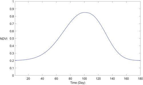Similarly, $x_4$ and $x_5$ determine the width and flatness of the left half. Asymmetric Gaussian is widely used in environmental research to depict phenological information of the vegetations (Jonsson and Eklundh 2002; Verbesselt et al. 2010). The length of NDVI time-series was assumed as 180 days for one season; $x_1$ was 110 and $x_2$ to $x_5$ were 42, 2, 38 and 2.5, respectively. The simulated clean NDVI time-series is shown in Figure 3.

Figure 3. Simulated clean NDVI time-series using asymmetric Gaussian function.

As mentioned, the sources of the noise were divided into low-value noise caused by clouds and shadows and random noises caused by other factors. Clouds represent one major factor affecting the quality of the NDVI time-series. Specifically, when one NDVI pixel is fully covered by cloud, the NDVI prefers to be a low outlier value. For MOD09 products, this type of noise can be effectively recorded by QC & QA flags (recorded as ‘cloudy’). Another type of low-value noise is mainly caused by cloud shadows. If the pixels are influenced by cloud shadows, the sensor can still receive vegetation reflectance information; however, the NDVI remains below the true value. These types of noise are usually recorded as ‘cloud shadow’ in QC & QA flags. In addition, previous research has indicated that ‘sub-pixel’ clouds may also exist in the NDVI time-series. The sub-pixel cloud noise occurs when clouds obscure only a portion of a pixel and may be ignored by QC & QA flags; thus, the image pixels recorded as ‘clear’ are still probably subject to their influence (Jönsson and Eklundh 2004; Takeshi et al. 2011).

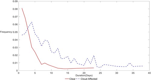
Based on these analyses, the simulated noise contained: (1) cloud coverage noise (low-value noise), (2) cloud shadow (low NDVI value noise), (3) sub-pixel clouds, which are not recorded in the simulated quality flag, and (4) other disturbance factors categorized as random noise. The MOD09GA QC & QA flags of the samples are driven to analyze the characteristics of the noise. In the 1991 selected samples, the pixels recorded as ‘clear,’ ‘cloudy,’ and other states, including ‘shadow,’ were 29.94%, 66.59%, and 3.47%, respectively. For cloud coverage noise, the frequency distribution of the cloud covered NDVI values is shown in Figure 4. Most of the cloud-affected NDVI values are <0.2. In the simulation experiment, the simulated cloud-covered NDVI values were generated randomly from the frequency distribution in the figure. For cloud shadows, as the NDVI values contained a portion of the real vegetation information, the simulated cloud-shadow-affected NDVI value can be generated by multiplying the simulated clean NDVI and cloud coverage rate (randomly generated ranging from 0 to 1). Thus, sub-pixel clouds and random instances of noise were also generated randomly and added to the simulated clean NDVI. Moreover, rainy weather may cause continuous cloud-covered NDVI in the simulated experiments. To simulate this phenomenon, the frequency distribution of the duration of the clear and the cloud-affected pixels were computed (Figure 5), and this frequency distribution was referred to as the generated simulated quality flag. The process of generating simulated one-day temporal resolution NDVI time-series is presented in Eq. (8): (8) $NDV{I}_s\left(t\right)=\{\begin{array}{c}\left(1-Q\left(t\right)\right)N_c\left(t\right)+Q\left(t\right)P\left(t\right)NDV{I}_{tr}\left(t\right)Q\left(t\right)=0,1\\ NDV{I}_{tr}\left(t\right)-N_{sc}\left(t\right)+N_r\left(t\right)Q\left(t\right)=2\end{array}$(8) where $N_c\left(t\right)$ is the cloud coverage noise at time $t$, $Q\left(t\right)$ is the quality flag, where the data influenced by cloud coverage noise are marked as 0, the data influenced by cloud shadow are marked as 1 and simulated ‘clear’ data are marked as 2; $P\left(t\right)$ determines the intensity of cloud shadow, ranging from 0 to 1; $NDV{I}_{tr}\left(t\right)$ is the simulated clean NDVI time-series; $N_{sc}\left(t\right)$ is the sub-pixel cloud noise, ranging from 0 to $v_1$ ($v_1\ge 0$), which satisfies the uniform distribution; and $N_r\left(t\right)$ is the random noise, ranging from $-v_2$ to $v_2$ ($v_2\ge 0$), satisfying uniform distribution as well.

Figure 4. Frequency distribution of the cloud covered NDVI value.

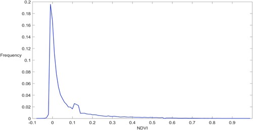
Figure 5. Frequency distribution of the duration of the pixel state (clear or cloud-affected).

The interaction between $N_{sc}$ and $N_r$ is complex. Many factors, such as the environment affecting vegetation growth, climate, and observation conditions, may influence their intensity, making it difficult to establish single best $v_1$ and $v_2$ values for simulations. Here, every possible pair of $v_1$ and $v_2$ was assessed to indicate the performance of the reconstruction method. The workflow of the simulated experiments is briefly introduced as follows (Figure 6):

1. $NDV{I}_{tr}$ was generated based on an asymmetric Gaussian function.

2. Randomly generated quality flags Q from the frequency distribution in Figure 5 were sorted temporally.

3. To simulate cloud coverage noise, random numbers were generated for $N_c$ based on the frequency distribution in Figure 4 and replaced the data in $NDV{I}_{tr}$ which are marked by $Q$ as influenced data.

4. Both $v_1$ of $N_{sc}$ and $v_2$ of $N_r$ ranged from 0 to 0.2, and every pair was analyzed at a step size of 0.01 to conduct the reconstruction experiments.

5. To conduct comparative experiments, all the experimental methods were used to reconstruct the simulated NDVI time-series. The experiments were repeated 30 times under every possible noise condition, and then the average AC (aAC) between simulated clean and reconstructed NDVI time-series was computed to evaluate method performance.

Figure 6. Workflow of the simulated experiment.

Certain factors, such as the rainy season, abandoned croplands, forest fires, and deforestation, may cause the NDVI values to deviate from the growing season and cause a ‘long-gap’ in the time-series. Thus, to analyze the influences of gaps in NDVI time-series on the reconstruction methods, artificial gaps were added into the simulated time-series ($N_{cs}$ and $N_r$ were both set to 0.05 to make sure the reconstruction algorithms were not significantly influenced by these instances of noise to evaluate their robustness to the time-series gap). The NDVI values of a certain duration (start and end date were randomly selected) were changed into continuous cloud coverage noise to generate gaps. The durations of continuous cloud coverage noises were 10, 20, 30, 60 and 90 days. The average aAC were computed to evaluate the response of the methods to the gaps.

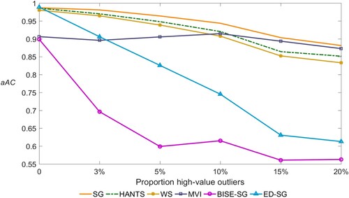
Another factor that may disturb the performance of the performance of the reconstruction method is the existence of high-value outliers. A similar simulated experiment was designed to analyze the influence of high-value outliers. We artificially added random outliers to the simulated NDVI timeseries (the value of the outlier randomly ranged from the simulated clean NDVI to 1, as those >1 were easily distinguished and eliminated) and computed the average aAC. The numbers of the high-value outliers were 3%, 5%, 10%, 15% and 20%.

2.3.4. Contrasting experiment on MOD09GQ-NDVI samples

Compared to the simulation experiments, the true NDVI time-series of different vegetation types are imperative to further understand the performance of the experimental reconstruction methods. From the selected samples, five landcover—evergreen needleleaf and broadleaf forests, deciduous broadleaf forests, herbaceous, and croplands—sample types were extracted, and their MOD09GQ-NDVIs were obtained for comparison. The characteristics of the reconstruction method were qualitatively evaluated based on their comparative graph, $a\delta$, and the average aNDVI (aaNDVI) of the samples.

2.3.5. Adaptation of ED-SG for multi-sensor NDVI time-series

Spatiotemporal resolution is one of the most significant attributes of NDVI time-series. For various remote sensing applications, selecting an appropriate resolution is critical to improve the precision and efficiency of data processing (Alexandridis, Gitas, and Silleos 2008; Kross et al. 2011). To verify the adaptation of ED-SG for different spatiotemporal resolutions of NDVI time-series, ED-SG was also employed on Sentinel-NDVI and Landsat-NDVI data for evaluation.

Notably, reconstruction experiments should be adjusted according to the dataset features: (1) In situations with multiple data points on the same day, the data with the best quality according to the QC & QA flag was selected as representative. If good-quality datapoints were >1 or equal to zero, they were replaced by their average (if there was no good-quality datapoint, the average of the bad-quality NDVI was used as representative NDVI). (2) The half-width of the smooth window of SG was adjusted to 10 NDVI values (50 days) for Sentinel-NDVI, and five NDVI values (80 days) for Landsat-NDVI.

2.3.6. Availability of ED-SG on GEE

Conventionally, large spatial scale, long-duration vegetation index time-series demand substantial storage and computational resources, limiting offline computing platforms’ availability. The development of GEE significantly improves the efficiency of complex vegetation index time-series computing. Accordingly, it has rapidly become one of the most popular platforms for remote sensing and environmental research. Due to its simplistic principles and stable reconstruction performance, ED-SG has the potential to integrate with GEE. To this end, ED-SG was programmed into GEE, and the MOD09GQ-NDVI values were reconstructed for the entire study area. The aNDVI of the reconstructed NDVI time-series were calculated seasonally (winter, Dec 2018–Feb 2019; spring, Mar 2019–May 2019; summer, Jun 2019–Aug 2019; fall, Sep 2019–Nov 2019). Previous research has indicated that aNDVI can reflect GPP of vegetation to a certain extent (Phillips, Hansen, and Flather 2008; Fu et al. 2014; Zhang et al. 2014); therefore, the aNDVI of the original MOD09GQ-NDVI was compared with the reconstructed MOD09GQ-NDVI, and average GPP (aGPP) derived from MOD17A2H GPP products to assess the performance of ED-SG on GEE. The aNDVI and aGPP of the selected samples were also extracted to test their correlation.

3. Results

3.1. The relation between $\mathit{\sigma }$ and reconstructed time-series

The $\sigma$-$a\delta$ graph (Figure 7) indicates that for MOD09GQ-NDVI, the $a\delta$ declined as $\sigma$ increased, yet the rate of decline gradually slowed. The $a\delta$ declined from 0.0046 to 0.0018 as $\sigma$ increased to 20 (∼61.3%), and then by 48.9% when increasing $\sigma$ to 100. REN showed a clear correlation with aδ, and the shape of their curve was similar to that of $\sigma$-aδ. REN declined from 0.6352 to 0.3206 (49.5%) when $\sigma$ was increased to 20 and further decreased by 18.8% to 0.2011 when $\sigma$ reached 100. 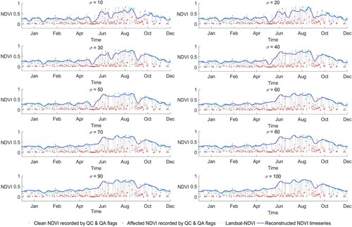Figure 8 illustrates the relationship between specific $\sigma$ values and the reconstructed time-series. When $\sigma$ was small, the noise remained in the reconstructed time-series, resulting in underestimated NDVI values. As $\sigma$ increased, the reconstruction quality improved, better fitting the upper envelope, and the missing data caused by continuous rainy weather were relatively fixed; however, when $\sigma$ increased further, the improvement of the reconstructed time-series was less obvious. Based on these analyses, $\sigma$ was set to 60 in the present study.

Figure 7. Relationship between $\sigma$-aδ, and $\sigma$-REN.

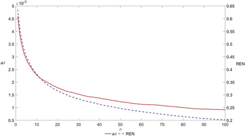
Figure 8. Reconstructed time-series under different $\sigma$ values.

3.2. Simulated reconstruction evaluation

The simulation results indicate that all reconstruction methods improved the aAC of the simulated NDVI time-series (Figure 9 and Table 3), with aACs values > 0.83. Specifically, when the intensities of both $N_{sc}$ and $N_r$ were weak and the simulated time-series were dominated by $N_c$, the aACs of all the contrasting methods were at a high level. As the intensities of $N_{sc}$ and $N_r$ were enhanced, the method performances began to differentiate. The aAC graphs of SG, HANTS, and WS appeared to be similar, and increasing $N_{sc}$ caused the aACs to decrease to <0.9; whereas the enhancement of $N_r$ did not significantly influence the aACs, which remained > 0.94. This implies that these three methods effectively suppressed random noise while remaining sensitive to instances of sub-pixel noise. MVI and ED-SG were similar in reconstruction performance, with average aAC and average variance that were significantly worse than in the other methods. The aAC graph also indicated that these two methods were sensitive to both sub-pixel cloud and random noise. ED-SG could adapt to most noise conditions, obtaining the best average aAC (0.9599) and low variance (0.0006). The aAC graph further indicated overall stability, with slight decreases in aAC observed in the upper-left portion of the graph when $N_{sc}$ is weak while $N_r$ is strong.

Figure 9. Resulting a AC. (a)aAC of original simulated NDVI time-series. (b) aAC of the experimental methods.

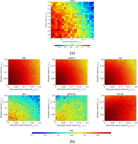
Table 3. Average aAC and variance of the experimental methods.

	Original	SG	HANTS	WS	MVI	BISE-SG	ED-SG
Average aAC	0.4733	0.9504	0.9439	0.9382	0.8418	0.8336	0.9599
Variance	0.0020	0.0010	0.0012	0.0012	0.0058	0.0066	0.0006

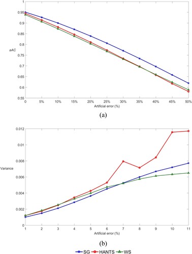
As mentioned, the SG filter and HANTS reference QC & QA flags to mask the low-quality data and clouds during pre-processing, and the WS must also refer to QC & QA flags to set the weight of $\lambda$ in this manner to avoid the influence of low-quality data and cloud coverage noise; however, some studies have highlighted the remaining uncertainties in the QC & QA flags of MODIS data (Motohka et al. 2009; Nagai et al. 2010; Hilker et al. 2012). The resulting good-quality NDVI points recorded as noise will thus not be effectively used by the algorithms, and the reconstructed time-series may miss pivotal phenological information, whereas the noise (particularly cloud coverage noise) recorded as good may alter the shape of the reconstructed time-series. To verify the influence of uncertainty, artificial errors were added into the simulated quality flag. The proportion of error ranged from 0 to 50% at 5% step increments. Figure 10 shows that the uncertainty of the QC & QA flags depressed the quality and stability of the reconstruction. As the artificial errors increased, the precision and stability of the methods markedly decreased. The average aAC (variance) of SG, HANTS, and WS decreased (increased) from 0.9503 (0.0010), 0.9439 (0.0012) and 0.9382 (0.0012) to 0.6191 (0.0077), 0.5802 (0.0117) and 0.5885 (0.0065), respectively. The influences on HANTS were relatively more significant, with variance exhibiting heavier volatility as the artificial errors increase.

Figure 10. (a) aAC and (b) variance of SG, HANTS, and WS after the addition of artificial errors.

Due to the different principles of the reconstruction methods, obvious differences in methods for the time-series gaps were detected (Figures 11 and 12). That is, SG, HANTS, and WS, which were designed to fit the NDVI time-series, were advantageous for filling the time-series gap. When the duration of the gap was low (10 days), the reconstruction NDVI time-series were similar to simulated NDVI time-series, with average aAC of SG, HANTS, and WS found to be 0.9873, 0.9817 and 0.9806 respectively. Compared to other reconstruction methods, SG exhibited the best robustness to the gaps in NDVI time-series when the duration of gaps was under 30 days, with average aAC > 0.98. LI of the data permits the GS filter to fill the low-value NDVI gaps. However, as the duration further increases, the gaps in NDVI time-series become too long to provide any effective values for the filter to fit. As the instances of noise recorded by the simulated quality flag have been masked, the reconstruction results become a straight line between the beginning and the end of the time-series gap. Similarly, missing continuous data tended to cause HANTS to collapse. In simulated experiments, when the duration of the time-series gap was larger than 20 days, HANTS would collapse and could not effectively repair such influence. Meanwhile, as an overall-fitting reconstruction method, WS could partially address differences in time-series gap; that is, the reconstruction time-series could restore the phenological features to a certain extent if the duration of gap was <30 days. However, as the duration increased, the reconstruction time-series exhibited obvious fluctuations and tended to underestimate the NDVI values.

Figure 11. The influences of time-series gaps on the reconstruction methods.

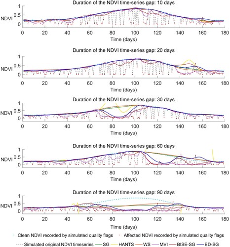
Figure 12. aAC of the reconstruction methods after the addition of time-series gap.

For the envelope extraction methods, MVI, BISE-SG and ED-SG tended to appear sunken as NDVI decreased, and their average aAC and variance were unsatisfactory as well. MVI is highly sensitive to continuously low NDVI values. Thus, in the simulated experiment, the continuous low noise values allowed MVI to reconstruct a smooth time-series. Alternatively, BISE-SG and ED-SG can be influenced by sporadic relatively high-value noise, causing the reconstructions to fluctuate. The fluctuations of ED-SG were heavier than those of BISE-SG.

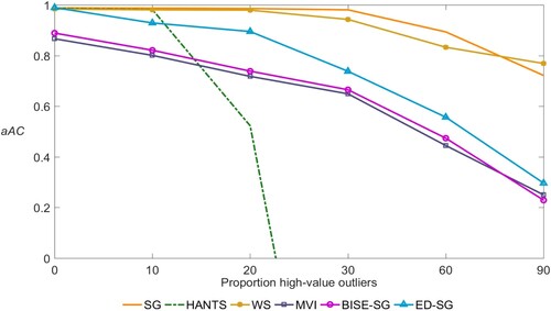
Figures 13 and 14 illustrate that the high-value outliers influence the performance of the reconstruction methods. SG, HANTS, and WS showed more robust to high-value outliers, whose aAC appeared more stable. When the proportion of the outliers increased to 20%, the aAC of these three methods are still >0.83 (0.8813 for SG, 0.8514 for HANTS, and 0.8331 for WS). From Figure 13, it is obvious that the fluctuations of these methods were also smaller than in the other three methods. The envelope extraction strategies are naturally sensitive to higher value datapoints. Thus, the reconstructions of BISE-SG, and ED-SG are badly influenced by the outliers, whose fluctuations are much severer and aAC decreased obviously. Of note, it is interesting that for MVI, as the high-value outlier became denser, the value of the outliers compensated for the low-value outliers caused by the simulated cloud influences, making the aAC increase when the proportion of the outliers was >10% (but Figure 13 obviously illustrates that the reconstructions were worse, not better). Another phenomenon is that in some cases, only a few outliers may have badly influenced the reconstruction results, as shown in Figure 13, Day 140, when the proportion of high-value outliers is 3%.

Figure 13. The influences of high-value outliers on the reconstruction methods.

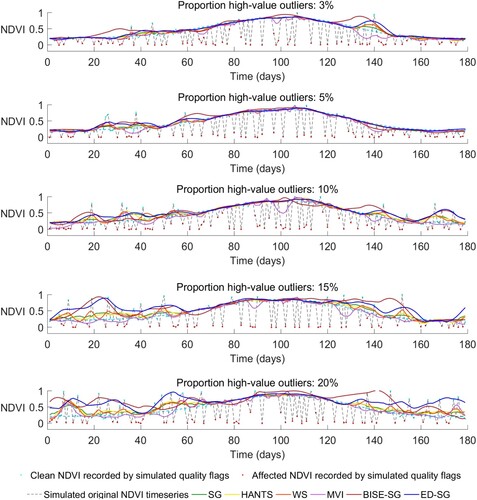
Figure 14. aAC of the reconstruction methods after the addition of high-value outliers.

3.3. MOD09GQ-NDVI reconstruction evaluations

The reconstructed MOD09GQ-NDVI of different types of vegetation are shown in Figure 15 and Table 4. The true NDVI time-series of evergreen needleleaf and broadleaf forests were stable with no obvious seasonal features. Alternatively, deciduous broadleaf and herbaceous forests were mostly single-season vegetation, with the growing season of the former (April to November) occurring slightly earlier than that of the latter (May to November). Cropland phenology is correlated with temperature and water resources, cultivation mode, and numerous other factors. Its NDVI time-series displayed multi-season features.

Figure 15. Reconstructed NDVI time-series of different vegetation types.

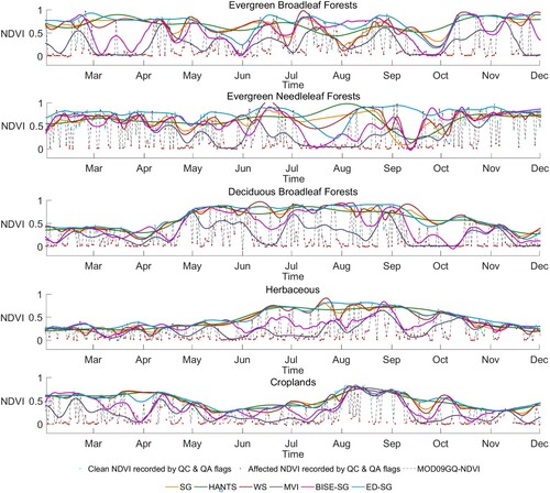
Table 4. $a\delta$ and aaNDVI of reconstructed time-series using MOD09GQ-NDVI samples.

		Evergreen Broadleaf Forests	Evergreen Needleleaf Forests	Deciduous Broadleaf Forests	Herbaceous	Croplands
aδ	Original	0.1884	0.2049	0.1864	0.1280	0.1559
	SG	0.0033	0.0041	0.0028	0.0027	0.0017
	HANTS	0.0007	0.0006	0.0003	0.0002	0.0003
	WS	0.0054	0.0069	0.0052	0.0047	0.0030
	MVI	0.0031	0.0030	0.0030	0.0018	0.0025
	BISE-SG	0.0053	0.0050	0.0051	0.0029	0.0040
	ED-SG	0.0019	0.0017	0.0012	0.0012	0.0013
aaNDVI	Original	0.2728	0.3233	0.2201	0.1911	0.2174
	SG	0.6636	0.6228	0.5583	0.3423	0.4995
	HANTS	0.6679	0.6304	0.5549	0.3452	0.5001
	WS	0.6654	0.6369	0.5498	0.3397	0.4966
	MVI	0.2999	0.3677	0.2573	0.2162	0.2585
	BISE-SG	0.4636	0.5092	0.4125	0.3194	0.3759
	ED-SG	0.6989	0.7022	0.6107	0.4178	0.5105

Other natural environment features, such as the soil, climate, and precipitation, can significantly increase the complexity of the noise over simulated experiments (Chen, Wang, and Fu 2020); however, the six contrasting methods were effective in NDVI time-series reconstruction. Compared to the original data, the $a\delta$s of the reconstructions decreased by approximately two orders of magnitude, and aaNDVI was higher. Seasonal vegetation was more likely to obtain smooth reconstruction results with lower $a\delta$s, whereas both types of evergreen vegetation tended to obtain higher aaNDVI values. Importantly, the NDVI time-series were often influenced by rainy season precipitation, producing consecutive low values lasting for tens of days or more and potentially causing a sudden drop in NDVI.

SG, HANTS, and WS obtained similar, smooth NDVI time-series reconstruction results with close aaNDVI values; however, the NDVI values were underestimated by the inclusions of low-value noise. The SG filter was robust to handle various noise conditions, and the method was somewhat effective in addressing missing data; however, the reconstructed time-series appeared to vibrate due to the residual noise. HANTS and WS adequately fit the time-series through all NDVI points, indicating that sporadic noise did not significantly influence the reconstructed results. HANTS maintained an obvious advantage in smoothing data ($a\delta$ < 0.001), but when the algorithm was conducted on the NDVI time-series with consecutive heavy noise, sudden drops appeared (e.g. evergreen needleleaf forests in September, Figure 15). A similar phenomenon also appeared in WS, where the influence of missing data was more noticeable. The reconstructed time-series of WS fluctuated severely when the consecutive instances of noise were masked, and aδ was also high (except for croplands, all other aδ were > 0.0045). MVI was unable to distinguish the noise from the original data during reconstruction. For MOD09GQ-NDVI data, dense noise resulted in the reconstructed time-series deviating from the true phenological trends, and the resulting aaNDVIs were rarely improved over the original NDVI time-series. The aaNDVI of evergreen needleleaf forests was 0.3677, with all others being ≤ 0.3. In principle, BISE lacks an effective strategy for dealing with consecutive instances of low-value noise, so the dense cloud coverage noise destabilized the BISE-SG reconstruction, yielding heavy vibrations and poor aδ and aaNDVI values. ED-SG performed the best among the methods, with the reconstructed time-series effectively restoring the upper envelope of the original, producing the highest aaNDVI. As the reconstructed NDVI time-series eliminated the influence of low-value noise, smoothness improved, and the aδ of ED-SG was secondary to HANTS (<0.002).

3.4. ED-SG and multi-sensor NDVI time-series

Compared to MOD09GQ-NDVI, Sentinel-NDVI and Landsat-NDVI have lower temporal resolutions and higher spatial resolutions. Lower temporal resolutions decrease NDVI time-series sensitivity to short-term phenological changes, and the longer-scale vegetation growth dominates the difference between adjacent NDVI points, thus reducing the vibration caused by random noise. Additionally, higher spatial resolution decreases the influence of sub- and mixed-pixel noise on NDVI time-series, therefore assisting with ED-SG noise removal.

Intuitively, for Sentinel-NDVI and Landsat-NDVI, the relationships between $a\delta$, REN, and $\sigma$ were consistent with MOD09GQ-NDVI. Because the difference between adjacent NDVI points was larger than that of MOD09GQ-NDVI, the derived aδ values of Sentinel-NDVI and Landsat-NDVI were higher. In addition, as the noise intensity was relatively low, more NDVI points were recognized as envelope nodes (higher REN, Figure 16). Accordingly, the $\sigma$ for these sensors required adjustment. Referring to the $\sigma$-$a\delta$, $\sigma$-REN graphs, and the reconstructed time-series samples under different $\sigma$ values (Figure 17), larger $\sigma$ values were set for Sentinel-NDVI (70), and Landsat-NDVI (85).

Figure 16. Relationships between $\sigma$-aδ and $\sigma$-REN for (a) Sentinel-NDVI and (b) Landsat-NDVI.

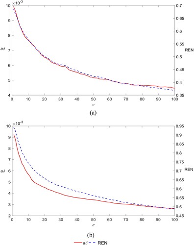
Figure 17. Reconstructed time-series for different $\sigma$ values using (a) Sentinel-NDVI and (b) Landsat-NDVI.

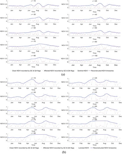
For true NDVI samples of different types of vegetation, as the intensity of the noise was significantly lower than that of MOD09GQ-NDVI, ED-SG was more effective at separating instances of noise and locating envelope nodes. The overall trends of the reconstruction results (Figure 18) and aaNDVI (Table 5) were similar to those of MOD09GQ as well. It was thus concluded that ED-SG showed adequate stability with NDVI time-series of different spatiotemporal resolutions, albeit at the sacrifice of phenological information at lower temporal resolutions. The duration between two adjacent NDVI points was larger, increasing the reconstructed roughness, and the aδ of the reconstructed NDVI time-series was larger as well. Compared to MOD09GQ-NDVI, the reconstructed results of Sentinel-NDVI yielded an increased aδ for the original and reconstructed NDVI time-series by 10.03% (deciduous broadleaf forests) ∼61.25% (evergreen broadleaf forests), and 210.52% (evergreen broadleaf forests) ∼538.46% (croplands). The aδ of the original and reconstructed NDVI time-series for Landsat-NDVI increased by 15.14% (herbaceous) ∼77.60.17% (evergreen broadleaf forests), and 376.47% (evergreen needleleaf forests) ∼1176.92% (croplands). In addition, there was a stronger influence of consecutive instances of low-value noise on the reconstruction (especially for Landsat-NDVI), and as the duration of missing data was inherently longer, the true phenology of the vegetation was more difficult to restore; therefore, low temporal resolution NDVI time-series (e.g. Landsat-NDVI) must be employed cautiously, prioritizing those applications requiring precision of date.

Figure 18. Reconstructed NDVI time-series of different vegetation types for (a) Sentinel-NDVI and (b) Landsat-NDVI.

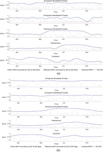
Table 5. $a\delta$ and aaNDVI of Sentinel-NDVI and Landsat-NDVI.

			Evergreen Broadleaf Forests	Evergreen Needleleaf Forests	Deciduous Broadleaf Forests	Herbaceous	Croplands
$a\delta$	Sentinel-NDVI	Origin	0.3038	0.2627	0.2051	0.1526	0.1893
		ED-SG	0.0059	0.0070	0.0055	0.0041	0.0083
	Landsat-NDVI	Origin	0.3346	0.2831	0.2489	0.1484	0.2061
		ED-SG	0.0104	0.0081	0.0098	0.0072	0.0166
aaNDVI	Sentinel-NDVI	Origin	0.2998	0.3345	0.2225	0.1799	0.2197
		ED-SG	0.7278	0.6648	0.5805	0.3427	0.4965
	Landsat-NDVI	Origin	0.4345	0.4477	0.3756	0.2243	0.4266
		ED-SG	0.7271	0.6959	0.5821	0.3464	0.5697

3.5. Evaluation of the ED-SG on GEE

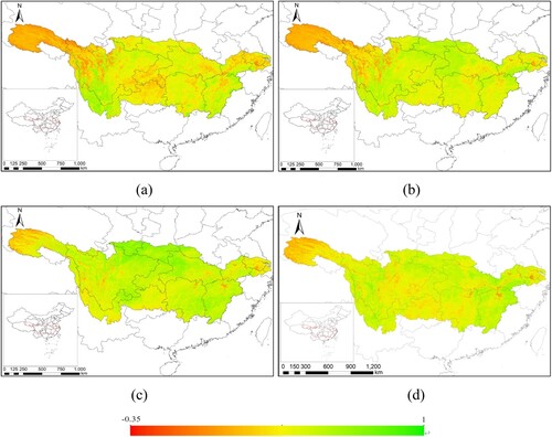
The influence of clouds and shadows can be seen in Figure 19. These instances of low-value noise caused the aNDVI of the original MOD09GQ-NDVI data to significantly underestimate the true NDVI. In Figure 19, aNDVI is relatively higher in the southeast during the winter and fall and increases in the middle and southeast during the spring and summer; however, the aNDVI of the original MOD09GQ-NDVI in most areas remained at a low level and did not express much seasonality. Following application of ED-SG, the average aNDVI of the four seasons increased from 0.1732 (winter), 0.2552 (spring), 0.2700 (summer), and 0.1929 (fall), to 0.4232 (winter), 0.4982 (spring), 0.5696 (summer), and 0.4678 (fall), indicating that ED-SG effectively addressed the influence of clouds and shadows. Accordingly, the true seasonal distribution of aNDVI is more clearly displayed in Figure 20. In the winter, the southwest and southeast Yangtze River Basin had larger aNDVI values (>0.5), yet the aNDVI in parts of the middle, and lower reaches of the Yangtze River were relatively lower (near 0). The NDVI of the whole area began to increase in the spring, reaching a summer peak where most areas in the north, central, and southeast of the study area maintained aNDVI > 0.6. The aNDVI gradually decreased in the fall, showing overall periodicity.

Figure 19. Seasonal aNDVI of original MOD09GQ-NDVI data: (a) winter, (b) spring, (c) summer, (d) fall.

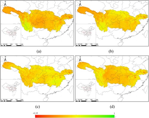
Figure 20. Seasonal aNDVI of reconstructed MOD09GQ-NDVI data using ED-SG: (a) winter, (b) spring, (c) summer, (d) fall.

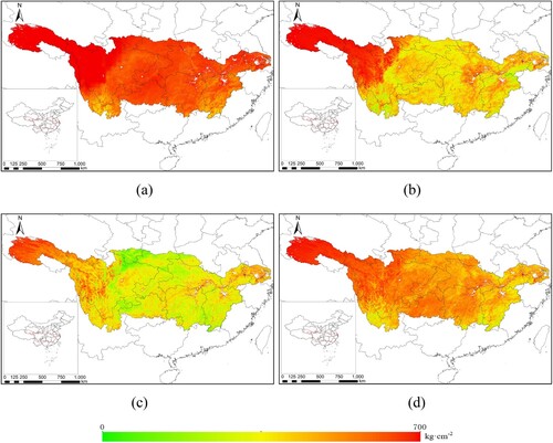
Similar patterns appeared in the distribution of aGPP (Figure 21), and the average seasonal aGPP were 87.4402 kg cm⁻² (winter), 336.6228 kg cm⁻² (spring), 423.3305 kg cm⁻² (summer), and 230.6018 kg cm⁻² (fall). aGPP in the winter was low, significantly increasing in the spring and summer, and decreasing in the fall. Generally, the spatial distribution of aGPP was similar to the distribution of the reconstructed aNDVI, only the seasonality of aGPP was more abundant than that of reconstructed aNDVI.

Figure 21. Seasonal aGPP of MOD17A2H GPP product: (a) winter, (b) spring, (c) summer, (d) fall.

ED-SG also improved the correlation between aNDVI and aGPP, and Figure 22 displays that the $r^2$ values for all four seasons were improved dramatically, from 0.0295 (winter), 0.0784 (spring), 0.2227 (summer), and 0.3089 (fall) to 0.2442 (winter), 0.2472 (spring), 0.5076 (summer), and 0.4010 (fall). Sample concentration increased as well, ultimately concluding that the NDVI time-series can improve GPP prediction after reconstruction via ED-SG; however, GPP more precisely reflects the initial daily total of photosynthesis, while spectral vegetation indices (e.g. NDVI) directly quantify the absorbed fraction of photosynthetically active radiation (FPAR) (Running and Zhao 2019). This difference may explain why $r^2$ never exceeded 0.5; moreover, when vegetation land cover was sparse, environmental factors (e.g. background soil reflectance) will influence NDVI more severely. Therefore, the $r^2$ and concentration of data in summer and fall, when the vegetation was most lush, outperformed those of the winter and spring. These results demonstrate that ED-SG is a reliable method for large spatiotemporal-scale NDVI time-series reconstruction using GEE.

Figure 22. Correlations between aNDVI and aGPP samples in the original and ED-SG corrected datasets: (a) winter, (b) spring, (c) summer, and (d) fall.

4. Discussion

In this study, we compared ED-SG to conventional NDVI time-series reconstruction methods through simulated experiments and qualitative analyses. The advantage of the simulated experiments is that the comparisons are implemented based on aAC between the simulated clean NDVI time-series generated by asymmetric Gaussian function, which to a certain extent avoids subjectivity, and it is helpful to analyze a certain influence on the reconstruction results while controlling the others. Of course, simulated experiments only abstracted the noises within the time-series into four types (cloud coverage noise, cloud shadow, sub-pixel clouds, and random noise), and the asymmetric Gaussian function only simulated one-season vegetation. The real long-duration satellite-based NDVI time-series are more complicated. Therefore, the qualitative analyses on real NDVI time-series are still indispensable.

The results of the contrasting analyses indicated that, owing to their specific assumptions and principles, each reconstruction method was adapted to different noise conditions. Notably, vegetation type did not directly influence the reconstructed results, and for most methods, the time-series with clear phenological features were more likely to produce stronger results. The noise conditions of high temporal resolution time-series, such as MOD09GQ-NDVI, were much more complicated, and the correlated time-series reconstruction was a considerable challenge. The reconstruction results of the SG filter, HANTS, and WS were similar, and they were more sensitive to random- than low-value noise. These methods tend to work better when the time-series has been pre-processed using the QC & QA flags. In addition, the reconstructed results were dependent on the precision of pre-processing and erroneously recorded NDVI values and residual sub-pixel cloud noise may have negatively influenced the quality of results. HANTS and WS reconstruction results produced smooth results, possibly aiding the subsequent extraction of phenological features, but the remaining low-value noise from the original time-series may underestimate NDVI. MVI was easier to realize, but hardly affected the time-series with overly dense noise. This method may be more adapted to pre-processed or lower temporal resolution NDVI time-series. The primary assumption behind BISE was that vegetative growth is stable, so it was unable to deal with time-series containing complex noise. For high temporal resolution NDVI time-series (e.g. MOD09GQ-NDVI), ED-SG tended to produce superior results, with the reconstructed NDVI time-series showing increased robustness and smoothness. The corresponding reconstructed time-series effectively eliminated noise.

Time-series gap and high-value outliers can disturb the reconstructions, no method can completely solve the problem. The NDVI time-series with a long duration of missing data did not provide sufficient references to generate meaningful reconstruction results. Fitting-data methods, such as SG, HANTS, and WS, performed relatively better at filling the gaps, however, as the features of time-series with gaps was more complex than normal time-series, the parameters of the algorithms should be reset to improve their generalization. Of note, the bad performances in aAC may not mean the reconstruction is useless when implemented on the NDVI time-series with time-series gaps, especially for MVI, BISE-SG, and ED-SG. If vegetation itself is damaged, the time-series will also appear collapsed. The reconstruction time-series should accurately reflect these gaps to express the damage to the vegetation, for which envelope extraction strategies such as MVI, BISE-SG, and ED-SG may be more appropriate. As for high-value outliers, when the outliers are denser, SG, HANTS, and WS are more suited because of their outlier-robustness, while the envelope strategies (MVI, BISE-SG and ED-SG) may be more sensitive to them.

With the exception for time-series gap and high-value outliers, another limitation of ED-SG is that the processing of setting $\sigma$ still a semi-empirical process. A small $\sigma$ will drive the discriminant function to decrease rapidly, resulting in more original data points identified as envelope nodes and enhanced accuracy of the reconstructed time-series; however, significant residual noise may remain. While larger $\sigma$ values tend to decrease the sensitivity of the discriminant function to low-value data points, the reconstructed time-series contains fewer envelope nodes, producing a smoother curve that better fits the upper envelope; however, too large of an $\sigma$ can preserve too few envelope nodes to contain adequate phenological information. Therefore, prior to ED-SG reconstruction, data features such as temporal resolution, weather conditions, and vegetation type should be considered and prior tests on the samples should be implemented to ensure the ED-SG has the best generalization.

5. Conclusions

In remote sensing applications, multiple uncertain factors influence the precision of NDVI time-series processing and computation. Here, a reconstruction method was proposed, combining envelope detection and the Savitzky-Golay filter, to improve the quality of NDVI time-series data. Its performance was assessed through simulations and true NDVI time-series reconstruction analyses, and the following results were obtained:

1. ED-SG can restore the upper envelope of high temporal resolution NDVI time-series well, and the smooth reconstructed NDVI time-series indicate the effective elimination of low-value noise.

2. Compared to conventional methods, ED-SG is more stable for high temporal resolution NDVI time-series. By setting the appropriate attenuation factor (σ), ED-SG can adapt to NDVI time-series of varying noise conditions, vegetation types, and spatiotemporal resolutions.

3. ED-SG can be programmed and conducted on the GEE platform to reconstruct NDVI over large spatiotemporal time-series. The results also showed a significant improvement in the correlation between aNDVI and aGPP.

In general, the method presented here has the potential to be widely accepted to provide smooth reconstructed NDVI time-series for vegetation growth monitoring, phenological feature extraction, crop mapping, and other subsequent remote sensing applications.

Acknowledgments

We thank Prof. Dongdong Kong and Mr. Benke Lou, whose open source code assisted with the reconstruction experiments on GEE platform. Thank Mr. Guoling Shen, who provided vital suggestions for this study. We also would like to thank Editage (www.editage.cn) for English language editing.

Data availability statement

Upon publication, the MODIS, Landsat and GFSAD30 Cropland Extent data products are available from the Land Processes Distributed Active Archive Center (LP DACC) (https://lpdaac.usgs.gov). Sentinel images are available from the European Space Agency (ESA, https://sentinels.copernicus.eu/web/sentinel). These remote sensing datasets presented in this manuscript are also available from Google Earth Engine (https://developers.google.com/earth-engine/datasets).

Disclosure statement

No potential conflict of interest was reported by the author(s).

Additional information

Funding

This study was supported by the National Key Research and Development Program of China (grant number 2017YFC1500501).

References

- Alexandridis, T. K., I. Z. Gitas, and N. G. Silleos. 2008. “An Estimation of the Optimum Temporal Resolution for Monitoring Vegetation Condition on a Nationwide Scale Using MODIS/Terra Data.” International Journal of Remote Sensing 29 (12): 3589–3607.
- Atzberger, Clement, and Paul H. C. Eilers. 2011a. “A Time Series for Monitoring Vegetation Activity and Phenology at 10-Daily Time Steps Covering Large Parts of South America.” International Journal of Digital Earth 4 (5): 365–386.
- Atzberger, Clement, and Paul H. C. Eilers. 2011b. “Evaluating the Effectiveness of Smoothing Algorithms in the Absence of Ground Reference Measurements.” International Journal of Remote Sensing 32 (13): 3689–3709.
- Brown, Molly. E., Jorge. E. Pinzón, Kamel Didan, Jeffrey T. Morisette, and Comton J. Tucker. 2006. “Evaluation of the Consistency of Long-Term NDVI Time Series Derived from AVHRR,SPOT-Vegetation, SeaWiFS, MODIS, and Landsat ETM+ Sensors.” IEEE Transactions on Geoence & Remote Sensing 44 (7):1787-1793.
- Chen, Jin, Per Jönsson, Masayuki Tamura, Zhihui Gu, Bunkei Matsushita, and Lars Eklundh. 2004. “A Simple Method for Reconstructing a High-Quality NDVI Time-Series Data set Based on the Savitzky–Golay Filter.” Remote Sensing of Environment 91 (3-4): 332–344.
- Chen, Zefeng, Weiguang Wang, and Jianyu Fu. 2020. “Vegetation Response to Precipitation Anomalies Under Different Climatic and Biogeographical Conditions in China.” Scientific Reports 10: 830. https://www.nature.com/articles/s41598-020-57910-1.
- Chen, Bangqian, Xiangming Xiao, Xiangping Li, Lianghao Pan, Russell Doughty, Jun Ma, Jinwei Dong, et al. 2017. “A Mangrove Forest map of China in 2015: Analysis of Time Series Landsat 7/8 and Sentinel-1A Imagery in Google Earth Engine Cloud Computing Platform.” ISPRS Journal of Photogrammetry and Remote Sensing 131: 104–120.
- Cihlar, Josef. 1996. “Identification of Contaminated Pixels in AVHRR Composite Images for Studies of Land Biosphere.” Remote Sensing of Environment 56 (3): 149–163.
- de Carvalho Júnior, Osmar Abílio, Renato Fontes Guimarães, Cristiano Rosa Silva, and Roberto Arnaldo Trancoso Gomes. 2015. “Standardized Time-Series and Interannual Phenological Deviation: New Techniques for Burned-Area Detection Using Long-Term MODIS-NBR Dataset.” Remote Sensing 7 (6): 6950–6985.
- de Jong, Rogier, Sytze de Bruin, Allard de Wit, Michael E. Schaepman, and David L. Dent. 2011. “Analysis of Monotonic Greening and Browning Trends from Global NDVI Time-Series.” Remote Sensing of Environment 115 (2): 692–702.
- Friedl, M. A., and D. Sulla-Menashe. 2015. MCD12Q1 MODIS/Terra+ Aqua Land Cover Type Yearly L3 Global 500m SIN Grid V006. edited by NASA EOSDIS Land Processes DAAC.
- Fu, Xinyu, Chuanjiang Tang, Xuxiao Zhang, Jingying Fu, and Dong Jiang. 2014. “An Improved Indicator of Simulated Grassland Production Based on MODIS NDVI and GPP Data: A Case Study in the Sichuan Province, China.” Ecological Indicators 40: 102–108.
- Gao, Feng, Yufang Jin, Crystal B. Schaaf, and Alan H. Strahler. 2002. “Bidirectional NDVI and Atmospherically Resistant BRDF Inversion for Vegetation Canopy.” IEEE Transactions on Geoence & Remote Sensing 40 (6): 1269–1278.
- Geerken, R., B. Zaitchik, and J. P. Evans. 2005. “Classifying Rangeland Vegetation Type and Coverage from NDVI Time Series Using Fourier Filtered Cycle Similarity.” International Journal of Remote Sensing 26 (24): 5535–5554.
- Gong, Pan, Zhongxin Chen, Huajun Tang, and Fengrong Zhang. 2006. Land Cover Classification Based on Multi-temporal MODIS NDVI and LST in Northeastern China.” IEEE International Symposium on Geoscience & Remote Sensing.
- Gorelick, Noel, Matt Hancher, Mike Dixon, Simon Ilyushchenko, David Thau, and Rebecca Moore. 2017. “Google Earth Engine: Planetary-Scale Geospatial Analysis for Everyone.” Remote Sensing of Environment 202: 18–27.
- Goward, Samuel N., Brian Markham, Dennis G. Dye, Wayne Dulaney, and Jingli Yang. 1991. “Normalized Difference Vegetation Index Measurements from the Advanced Very High Resolution Radiometer.” Remote Sensing of Environment 35 (2-3): 257–277.
- Gu, Yingxin, Jesslyn F. Brown, James P. Verdin, and Brian Wardlow. 2007. “A Five-Year Analysis of MODIS NDVI and NDWI for Grassland Drought Assessment Over the Central Great Plains of the United States.” Geophysical Research Letters 34 (6): 1–6.
- Gumma, Murali Krishna, Prasad S. Thenkabail, Pardhasaradhi G. Teluguntla, Adam Oliphant, Jun Xiong, Chandra Giri, Vineetha Pyla, Sreenath Dixit, and Anthony M. Whitbread. 2020. “Agricultural Cropland Extent and Areas of South Asia Derived Using Landsat Satellite 30-m Time-Series big-Data Using Random Forest Machine Learning Algorithms on the Google Earth Engine Cloud.” GIScience & Remote Sensing 57 (3): 302–322.
- Hilker, Thomas, Alexei I. Lyapustin, Compton J. Tucker, Piers J. Sellers, Forrest G. Hall, and Yujie Wang. 2012. “Remote Sensing of Tropical Ecosystems: Atmospheric Correction and Cloud Masking Matter.” Remote Sensing of Environment 127: 370–384.
- Hird, Jennifer N., and Gregory J. McDermid. 2009. “Noise Reduction of NDVI Time Series: An Empirical Comparison of Selected Techniques.” Remote Sensing of Environment 113 (1): 248–258.
- Hmimina, G., E. Dufrene, J. Y. Pontailler, N. Delpierre, M. Aubinet, B. Caquet, A. de Grandcourt, et al. 2013. “Evaluation of the Potential of MODIS Satellite Data to Predict Vegetation Phenology in Different Biomes: An Investigation Using Ground-Based NDVI Measurements.” Remote Sensing of Environment 132: 145–158.
- Holben, Brent N. 1986. “Characteristics of Maximum-Value Composite Images from Temporal AVHRR Data.” International Journal of Remote Sensing 7 (11): 1417–1434.
- Huete, Alfredo R., and Hhui Qing Liu. 1994. “An Error and Sensitivity Analysis of the Atmospheric- and Soil-Correcting Variants of the NDVI for the MODIS-EOS.” IEEE Transactions on Geoence & Remote Sensing 32 (4): 897–905.
- Ji, Lei, and Kevin Gallo. 2015. “An Agreement Coefficient for Image Comparison.” Photogrammetric Engineering & Remote Sensing 73 (7): 823–833.
- Ji, Lei, and Albert J. Peters. 2003. “Assessing Vegetation Response to Drought in the Northern Great Plains Using Vegetation and Drought Indices.” Remote Sensing of Environment 87 (1): 85–98.
- Jin, Yuhao, Xiaoping Liu, Yimin Chen, and Xun Liang. 2018. “Land-cover Mapping Using Random Forest Classification and Incorporating NDVI Time-Series and Texture: A Case Study of Central Shandong.” International Journal of Remote Sensing 39 (23): 8703–8723.
- Jonsson, P., and L. Eklundh. 2002. “Seasonality Extraction by Function Fitting to Time-Series of Satellite Sensor Data.” IEEE Transactions on Geoscience and Remote Sensing 40 (8): 1824–1832.
- Jönsson, Per, and Lars Eklundh. 2004. “TIMESAT—a Program for Analyzing Time-Series of Satellite Sensor Data.” Computers & Geosciences 30 (8): 833–845.
- Julien, Yves, and José A. Sobrino. 2010. “Comparison of Cloud-Reconstruction Methods for Time Series of Composite NDVI Data.” Remote Sensing of Environment 114: 618–625.
- Kandasamy, S., F. Baret, A. Verger, P. Neveux, and M. Weiss. 2013. “A Comparison of Methods for Smoothing and gap Filling Time Series of Remote Sensing Observations – Application to MODIS LAI Products.” Biogeosciences (online) 10: 4055–4071.
- Kong, Dongdong, Yongqiang Zhang, Xihui Gu, and Dagang Wang. 2019. “A Robust Method for Reconstructing Global MODIS EVI Time Series on the Google Earth Engine.” ISPRS Journal of Photogrammetry and Remote Sensing 155: 13–24.
- Kowalski, Katja, Cornelius Senf, Patrick Hostert, and Dirk Pflugmacher. 2020. “Characterizing Spring Phenology of Temperate Broadleaf Forests Using Landsat and Sentinel-2 Time Series.” International Journal of Applied Earth Observation and Geoinformation 92: 102172. https://www.sciencedirect.com/science/article/pii/S0303243419312164.
- Kross, Angela, Richard Fernandes, Jonathan Seaquist, and Elisabeth Beaubien. 2011. “The Effect of the Temporal Resolution of NDVI Data on Season Onset Dates and Trends Across Canadian Broadleaf Forests.” Remote Sensing of Environment 115: 1564–1575.
- Li, Congcong, Hongjun Li, Jiazhen Li, Yuping Lei, Chunqiang Li, Kiril Manevski, and Yanjun Shen. 2019. “Using NDVI Percentiles to Monitor Real-Time Crop Growth.” Computers and Electronics in Agriculture 162: 357–363.
- Li, Feng, Guo Song, Zhu Liujun, Zhou Yanan, and Lu Di. 2017. “Urban Vegetation Phenology Analysis Using High Spatio-Temporal NDVI Time Series.” Urban Forestry & Urban Greening 25: 43–57.
- Liu, Xinkai, Han Zhai, Yonglin Shen, Lou Benke, Changmin Jiang, Tianqi Li, Sayed Bilal Hussain, and Guoling Shen. 2020. “Large-Scale Crop Mapping from Multisource Remote Sensing Images in Google Earth Engine.” IEEE Journal of Selected Topics in Applied Earth Observations and Remote Sensing 13: 414–427.
- Liu, Chong, Qi Zhang, Shiqi Tao, Jiaguo Qi, Mingjun Ding, Qihui Guan, Bingfang Wu, et al. 2020. “A new Framework to map Fine Resolution Cropping Intensity Across the Globe: Algorithm, Validation, and Implication.” Remote Sensing of Environment 251: 1112095. https://www.sciencedirect.com/science/article/abs/pii/S0034425720304685.
- Lovell, J. L., and R. D. Graetz. 2001. “Filtering Pathfinder AVHRR Land NDVI Data for Australia.” International Journal of Remote Sensing 22 (13): 2649–2654.
- Ma, Lei, Liang Cheng, Manchun Li, Yongxue Liu, and Xiaoxue Ma. 2015. “Training set Size, Scale, and Features in Geographic Object-Based Image Analysis of Very High Resolution Unmanned Aerial Vehicle Imagery.” ISPRS Journal of Photogrammetry and Remote Sensing 102: 14–27.
- Ma, Mingguo, and Frank Veroustraete. 2006. “Reconstructing Pathfinder AVHRR Land NDVI Time-Series Data for the Northwest of China.” Advances in Space Research 37 (4): 835–840.
- Motohka, T., K. N. Nasahara, A. Miyata, M. Mano, and S. Tsuchida. 2009. “Evaluation of Optical Satellite Remote Sensing for Rice Paddy Phenology in Monsoon Asia Using a Continuous in Situ Dataset.” International Journal of Remote Sensing 30 (17): 4343–4357.
- Nagai, Shin, Rnnobuko Saigusa, Rnhiroyuki Muraoka, and Kenlo Nishida Nasahara. 2010. “What Makes the Satellite-Based EVI–GPP Relationship Unclear in a Deciduous Broad-Leaved Forest?” Ecological Research 25 (2): 359–365.
- Oliphant, A. J., P. S. Thenkabail, P. Teluguntla, J. Xiong, R. G. Congalton, K. Yadav, R. Massey, M. K. Gumma, and C. Smith. 2017. NASA Making Earth System Data Records for Use in Research Environments (MEaSUREs) Global Food Security-Support Analysis Data (GFSAD) Cropland Extent 2015 Southeast Asia 30m. Sioux Falls, SD, USA: USGS EROS.
- Parente, Leandro, Vinícius Mesquita, Fausto Miziara, Luis Baumann, and Laerte Ferreira. 2019. “Assessing the Pasturelands and Livestock Dynamics in Brazil, from 1985 to 2017: A Novel Approach Based on High Spatial Resolution Imagery and Google Earth Engine Cloud Computing.” Remote Sensing of Environment 232: 111301. https://www.sciencedirect.com/science/article/abs/pii/S0034425719303207.
- Phillips, Linda B., Andrew J. Hansen, and Curtis H. Flather. 2008. “Evaluating the Species Energy Relationship with the Newest Measures of Ecosystem Energy: NDVI Versus MODIS Primary Production.” Remote Sensing of Environment 112 (12): 4381–4392.
- Qu, Sai, Lunche Wang, Aiwen Lin, Deqing Yu, Moxi Yuan, and Chang’an Li. 2020. “Distinguishing the Impacts of Climate Change and Anthropogenic Factors on Vegetation Dynamics in the Yangtze River Basin, China.” Ecological Indicators 108: 105724. https://www.sciencedirect.com/science/article/abs/pii/S1470160X19307174.
- Running, Steven W., and Maosheng Zhao. 2019. User’s Guide Daily GPP and Annual NPP (MOD17A2H/A3H) and Year-end Gap-Filled (MOD17A2HGF/A3HGF) Products NASA Earth Observing System MODIS Land Algorithm (For Collection 6): MODIS Land Team.
- Savitzky, Abraham, and M. J. E. Golay. 1964. “Smoothing and Differentiation of Data by Simplified Least Squares Procedures.” Analytical Chemistry 36 (8): 1627–1639.
- Sulla-Menashe, Damien, and Mark A. Friedl. 2018. User Guide to Collection 6 MODIS Land Cover (MCD12Q1 and MCD12C1) Product. Sioux Falls, SD: USGS.
- Sun, Rui, Shaohui Chen, Hongbo Su, Chunrong Mi, and Ning Jin. 2019. “The Effect of NDVI Time Series Density Derived from Spatiotemporal Fusion of Multisource Remote Sensing Data on Crop Classification Accuracy.” International Journal of Geo-Information 8 (11): 502–518.
- Sun, Chao, Sergio Fagherazzi, and Yongxue Liu. 2018. “Classification Mapping of Salt Marsh Vegetation by Flexible Monthly NDVI Time-Series Using Landsat Imagery.” Estuarine Coastal and Shelf Science 213 (30): 61–80.
- Takeshi, Motohka, Nasahara Kenlo Nishida, Murakami Kazutaka, and Nagai Shin. 2011. “Evaluation of Sub-Pixel Cloud Noises on MODIS Daily Spectral Indices Based on in Situ Measurements.” Remote Sensing 3: 1644–1662.
- Teluguntla, Pardhasaradhi, Prasad S. Thenkabail, Adam Oliphant, Jun Xiong, Murali Krishna Gumma, Russell G. Congalton, Kamini Yadav, and Alfredo Huete. 2018. “A 30-m Landsat-Derived Cropland Extent Product of Australia and China Using Random Forest Machine Learning Algorithm on Google Earth Engine Cloud Computing Platform.” ISPRS Journal of Photogrammetry and Remote Sensing 144: 325–340.
- Teluguntla, P., P. S. Thenkabail, J. Xiong, M. K. Gumma, R. G. Congalton, A. J. Oliphant, T. Sankey, et al. 2017. NASA Making Earth System Data Records for Use in Research Environments (MEaSUREs) Global Food Security-support Analysis Data (GFSAD) @30-m for Australia, New Zealand, China, and Mongolia: Cropland Extent Product (GFSAD30AUNZCNMOCE). edited by NASA EOSDIS Land Processes DAAC.
- Verbesselt, Jan, Rob Hyndman, Glenn Newnham, and Darius Culvenor. 2010. “Detecting Trend and Seasonal Changes in Satellite Image Time Series.” Remote Sensing of Environment 114 (1): 106–115.
- Verger, Aleixandre, Frédéric Baret, and Marie Weiss. 2016. “A Multisensor Fusion Approach to Improve LAI Time Series.” Remote Sensing of Environment 115: 2460–2470.
- Vermote, Eric F, Nazmi Z. El Saleous, and Christopher O. Justice. 2002. “Atmospheric Correction of MODIS Data in the Visible to Middle Infrared: First Results.” Remote Sensing of Environment 83 (1-2): 97–111.
- Viovy, N., O. Arino, and A. S. Belward. 1992. “The Best Index Slope Extraction (BISE): A method for reducing noise in NDVI time-series.” International Journal of Remote Sensing 13 (8): 1585–1590.
- Vrieling, A., K. M. de Beurs, and M. E. Brown. 2011. “Variability of African Farming Systems from Phenological Analysis of NDVI Time Series.” Climatic Change 109: 455–477.
- Wei, Wen, Yuanpin Chang, and Zhijun Dai. 2014. “Streamflow Changes of the Changjiang (Yangtze) River in the Recent 60 Years: Impacts of the East Asian Summer Monsoon, ENSO, and Human Activities.” Quaternary International 336: 98–107.
- Weiss, Marie, Frédéric Baret, Sébastien Garrigues, and Roselyne Lacaze. 2007. “LAI and fAPAR CYCLOPES Global Products Derived from VEGETATION. Part 2: Validation and Comparison with MODIS Collection 4 Products.” Remote Sensing of Environment 110 (3): 317–331.
- Whittaker, E. T. 1922. “On a new Method of Graduation.” Proceedings of the Edinburgh Mathematical Mathematical 41: 63–75.
- Xu, Jijun, Dawen Yang, Yonghong Yi, Zhidong Lei, Chen Jin, and Wenjun Yang. 2008. “Spatial and Temporal Variation of Runoff in the Yangtze River Basin During the Past 40 Years.” Quaternary International 186: 23–42.
- Yang, Gang, Huanfeng Shen, Liangpei Zhang, Zongyi He, and Xinghua Li. 2015. “A Moving Weighted Harmonic Analysis Method for Reconstructing High-Quality SPOT VEGETATION NDVI Time-Series Data.” IEEE Transactions on Geoscience & Remote Sensing 53 (11): 6008–6021.
- Yang, Yongke, Pengfeng Xiao, Xuezhi Feng, and Haixing Li. 2017. “Accuracy Assessment of Seven Global Land Cover Datasets Over China.” ISPRS Journal of Photogrammetry Remote Sensing 125: 156–173.
- Zhang, Qingyuan, Yenben Cheng, Alexei I. Lyapustin, Yujie Wang, Xiangming Xiao, Andrew Suyker, Shashi Verma, Bin Tan, and Elizabeth M. Middleton. 2014. “Estimation of Crop Gross Primary Production (GPP): I. Impact of MODIS Observation Footprint and Impact of Vegetation BRDF Characteristics.” Agricultural and Forest Meteorology 191: 51–63.
- Zhao, Hu, Zhengwei Yang, Liping Di, Lin Li, and Haihong Zhu. 2009. “Crop Phenology Date Estimation Based on NDVI Derived from the Reconstructed MODIS Daily Surface Reflectance Data.” GIScience & Remote Sensing 56 (2): 1–6.
- Zhou, Jie, Li Jia, and Massimo Menenti. 2015. “Reconstruction of Global MODIS NDVI Time Series: Performance of Harmonic ANalysis of Time Series (HANTS).” Remote Sensing of Environment 163: 217–228.
- Zhu, Xiaolin, Jin Chen, Feng Gao, Xuehong Chen, and Jeffrey G. Masek. 2010. “An Enhanced Spatial and Temporal Adaptive Reflectance Fusion Model for Complex Heterogeneous Regions.” Remote Sensing of Environment 114: 2610–2623.