Health assessment of plantations based on LiDAR canopy spatial structure parameters

ABSTRACT

The Yellow River Delta (YRD) has China's largest artificial Robinia pseudoacacia forest, which was planted in the late 1970s and suffered extensive dieback in the 1990s. The health grade of the R.pseudoacacia forest (named canopy vigor grade, CVG) could be achieved by using high-resolution images and canopy vigor indicators (CVIs). However, a previous study showed that there was no significant correlation between CVG and the field-estimated aboveground biomass (AGB) of R.pseudoacacia forest. Therefore, this study aims to construct forest health indicators (FHIs) based on canopy spatial structure parameters extracted from LiDAR. The FHIs included Weibull_α (the scale parameter of the Weibull density function that reflects the shape of the tree canopy), VCI (vertical complexity index), sdCC (the standard deviation of canopy cover), H₉₉ (the 99th percentile height) and cvLAD (the coefficient of variation of leaf area density), and could significantly distinguish three forest health grades (FHG) (p < 0.05). The FHG was positively correlated with forest AGB (r_s = 0.51, p = 0.004), and the similarity value with CVG was 63.33%. The results of this study confirmed that the FHIs can reflect both canopy vigor and tree productivity, and distinguish forest health status without prior classification information.

KEYWORDS:

• Forest health indicators
• LiDAR
• structural parameter
• Robinia pseudoacacia forest
• the Yellow River Delta

1. Introduction

As the main body of terrestrial ecosystems, forests play a key role in both the global carbon cycle and climate change mitigation (Pan et al. 2011). Forests are degrading and even disappearing at an alarming rate worldwide (Hansen et al. 2013). Planted forests are the priority choice for the management of degraded ecosystems, which can prevent wind and fix sand, maintain soil and water loss and improve saline soil (Jiang, Zhu, and Zeng 2003). Planted forests account for approximately 7% of the world's total forest area, of which China’s planted forests account for 6.9×107 ha, which ranks China first in the world (FAO 2020). However, since the 1990s, the growth and development of planted forests in China have been stagnating and even dying, which has greatly reduced the carbon storage of forests (Jiang, Zhu, and Zeng 2003; Zhu et al. 2005). Therefore, the rapid and accurate assessment of the health status of plantations is helpful for sustainable forest management and carbon sequestration of terrestrial forest ecosystems.

The study of forest health has a long history; however, there is still no universal evaluation system for forest health (Lausch et al. 2016). The United States Forest Service (USFS) has been responsible for implementing nationwide field-based forest health monitoring, covering canopy, soil, vegetation diversity, and lichen communities (Woodall et al. 2011). In Europe, forest health is concerned with the impact of climate change on forests, with indicators including biological and environmental factors and the resilience and sustainability of forest ecosystems (Bussotti and Pollastrini 2017). Thus, the forest health indicator may vary by scale or by forest use or disturbance/stress type (Arnott et al. 2015; Pause et al. 2016).

On the tree scale, a healthy tree is generally defined as a tree that is free of diseases, while over an extensive area, such as on the stand and landscape scale, forest health status is difficult to assess (Trumbore, Brando, and Hartmann 2015). Since signs of forest degradation are usually observed in the tree canopy, indicators representing canopy conditions are widely used for forest health assessments at the stand level (Lausch et al. 2016). This visual assessment of the canopy reflects the canopy vigor: large, dense canopy has great vitality (Kramer 1966). The canopy vigor can be assessed using five canopy vigor indicators (CVIs) proposed by the USFS, including live crown ratio, crown density, crown diameter, crown dieback, and foliar transparency (Schomaker et al. 2007). But such canopy vigor grade (CVG), derived from tree appearance, is not a complete representation of forest health. For example, in a stand with overgrown weeds, the growth of tree height and diameter at breast height (DBH) will be affected by stand density (Chen and Brockway 2017), but the canopy may still show vigor characteristics, such as green leaves, full foliage, and low frequency of insect and disease (Grulke et al. 2020). Photosynthesis in these structurally damaged trees was weak compared to other tall trees of the same age. Photosynthesis is theoretically the most suitable indicator of tree productivity. But measuring photosynthetic rates requires precise measurements and expensive equipment, so biomass, the carbon fixed through photosynthesis, is often used in forest monitoring (Cherubini, Battipaglia, and Innes 2021; Marco 1997). The Yellow River Delta (YRD) has the largest artificial R.pseudoacacia forest in China. In the previous study, the health status of R.pseudoacacia forest was divided into three CVGs: healthy, medium dieback, and severe dieback, using five CVIs combined with IKONOS high-resolution image (Wang et al. 2015). However, another study found that the CVGs of the R.pseudoacacia forest has no relationship with the field-estimated aboveground biomass (AGB) (Lu et al. 2020), indicating that CVIs could not represent tree productivity. Therefore, it is urgent to establish a forest health indicator system that reflects both tree productivity and canopy vigor.

Forest health is commonly assessed via field surveys and remote sensing (Lausch et al. 2017). In field surveys, forest health conditions have been evaluated using a combination of different kinds of indicators (Potter and Conkling 2016). However, collecting the corresponding information over large areas is connected to laborious and expensive field campaigns. As an alternative, optical remote sensing can realize the rapid monitoring of forest health (Smigaj et al. 2019). Environmental stresses such as water, salt, and drought will change the biochemical parameters of leaves, such as nitrogen concentration, photosynthetic pigment, and water content, thus leading to corresponding changes in the remote sensing spectrum and vegetation index (Asner et al. 2004; Cammarano et al. 2015; Eitel et al. 2011; Huesca et al. 2019). However, these indicators often reflect the horizontal surface of the canopy and cannot express the structure of the tree canopy and the understory. Disturbance/stress not only discolors leaves and reduces water content but also causes significant changes in stand structure, such as increased forest gap and uneven vertical distribution of leaves, due to falling leaves and branches (Coops et al. 2009; Zarnoch, Bechtold, and Stolte 2004). In addition, when disease damage to trees spreads upward from the lower part of the canopy, optical remote sensing alone cannot detect when and how severe the infection is (Smigaj et al. 2019). Therefore, quantifying canopy spatial structure is very important for the accurate assessment of forest health.

Due to strong canopy penetration, LiDAR (light detection and ranging) can obtain three-dimensional forest structures within and below the canopy (Næsset 2002). Therefore, LiDAR is well suited for measuring forest biophysical parameters, such as tree height, volume, and biomass (Lausch et al. 2017), whose changes can reflect tree growth (Næsset and Gobakken 2008; Silva et al. 2016). LiDAR can also easily calculate a variety of parameters that describe forest ecological conditions, the most critical of which is canopy cover (Lausch et al. 2017; Leeuwen and Nieuwenhuis 2010). The vertical distribution differences of branches and leaves in the canopy can be distinguished by quantifying the canopy profile with a Weibull distribution (Tompalski et al. 2015). In addition, LiDAR-derived structural parameters can describe both the vertical (Zhang, Lin, and She 2017) and horizontal heterogeneity (Moran, Rowell, and Seielstad 2018) of stands, which have a close bearing on forest health and biodiversity (Gao et al. 2014). In summary, the LiDAR-derived parameters can well represent the changes in canopy spatial structure and therefore quantitatively evaluate the forest health status.

The purpose of this study is to realize automatic and rapid identification of forest health status using structural parameters extracted from LiDAR without prior classification information. The proposed FHI system is expected to comprehensively reflect canopy vigor and forest productivity.

2. Materials and methods

2.1. Study area

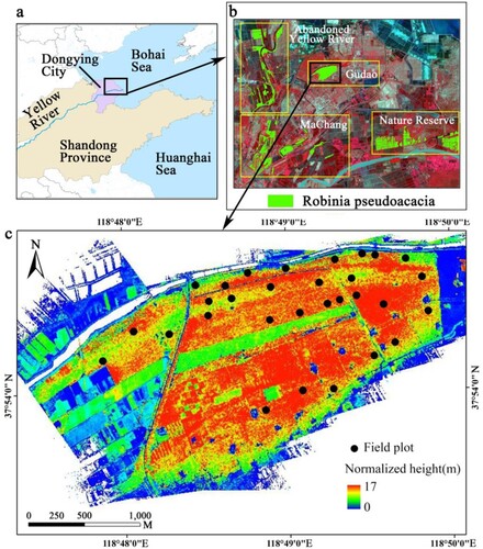
The YRD is located on the east coast of China (Figure 1a) and has a warm temperate subhumid continental monsoon climate. It has a shallow water table, low soil productivity, and widespread saline soil (Wu, Liu, and Huang 2016). Because of the characteristics of nitrogen fixation, the prevention of soil erosion, and salt tolerance, R.pseudoacacia trees have been planted as the main afforestation tree species in the YRD since the 1970s. However, since the 1990s, these trees have suffered from many diebacks and even deaths. Up to 2013, four R.pseudoacacia forests (Figure 1b) covered a total area of 27.94 km², of which 41.46% were healthy, 36.09% suffered from medium dieback and the remaining 22.45% from severe dieback or were completely dead (Wang et al. 2015). The Gudao forest, with a total area of 5 km², was selected as our study area (Figure 1c). The forests are mostly pure stands of mature stands with tree spacing ranging from 3 m to 4 m. The forest structure is simple, with herbaceous species in the understory.

Figure 1. Location of the study area. (a) The Yellow River Delta. (b) Four R.pseudoacacia forest areas shown in a Landsat 8 OLI image obtained in June 2017. (c) The Gudao forest with the background height from point cloud Lidar data obtained in June 2017.

2.2. Datasets

2.2.1. UAV-LiDAR data

The LiDAR point cloud data were acquired in June 2017 using the Li-Air airborne LiDAR System (GreenValley, China), which was equipped with a Riegl VUX-1 four-return laser scanner, an IMU (Novatel), and a dual frequency GPS (Novatel). An eight-rotor UAV platform was flying at 120 m above the ground with a ground speed of 4.8 m·s⁻¹ and a cruising radius of 2 km. The average point density was 70 m⁻² with a ranging accuracy of 10 mm, and the spot diameter was approximately 50 mm. The acquired data were georeferenced to the UTM coordinate system (geodatum: WGS84).

2.2.2. Field data

Similar to a previous two-level sampling design (Wang et al. 2015), samples were collected at two levels, namely, 30 m × 30 and 10 m × 10 m. In each 30 m × 30 m plot, five 10 m × 10 m subplots were arranged, deployed in the four corners and one at the center. The geographic coordinates of these plots were recorded with the GEOXT6000 GPS (Trimble Navigation Company) locator. In each subplot, we selected one standard tree and evaluated the five CVIs (Table 1) referring to the Crown Condition Classification Guide (Schomaker et al. 2007). The live crown ratio was measured by the ratio of live crown to tree height. The crown diameter was expressed by the ratio of the crown diameter to the healthy trees of the same species. Visually reconstruct damaged or missing crown outline by comparing crowns of healthy trees of the same species. Then determine the crown dieback by assessing what percentage of the outlined area is dieback. The crown density and foliar transparency were estimated based on the crown density-foliage transparency card that proposed by the USFS. The card provides a table of percentages for various combinations of density and transparency. For each plot, the indicators were obtained by averaging the five standard trees, and each indicator was classified as Class 1, 2, or 3 based on the thresholds. Finally, the CVG at the plot level was determined by specific rules (Table 2). Tables 1 and 2 refer to the previous studies (Wang et al. 2015). A total of 30 field plots (the black dots in Figure 1c) were investigated in June 2017, June 2019, and October 2019, including 14 healthy plots, 10 medium dieback plots, and 6 severe dieback plots. The stand conditions for 2017 and 2019 are the same, because the R.pseudoacacia forest in this study is mature forest, the growth of trees basically stopped.

Table 1. The canopy vigor indicators and classification thresholds.

Indicator	Class 1	Class 2	Class 3
Live crown ratio (%)	>40	20∼35	5∼15
Crown diameter (%)	>55	26∼54	1∼25
Crown density (%)	>55	25∼50	5∼20
Crown dieback (%)	0∼5	10∼25	>30
Foliar transparency (%)	0∼45	50∼70	>75

Table 2. Rules for determining the CVG based on canopy vigor indicator.

Grade	The number of the indicator classification
Healthy (h)	All indicators are Class 1, or only one Class 2 but not Class 3.
Medium dieback (m)	All indicators are Class 2, or only one Class 1, or only one Class 3.
Severe dieback (s)	All indicators are Class 3, or only one Class 2.

Height and DBH were measured for all trees in the above plot. Tree height was determined by Vertex IV and Vertex Laser Geo (Haglöf Sweden AB, Långsele, Sweden), and tree DBH was measured at 1.3 m above the ground with a tape measure. The plot-level forest AGB was derived from all trees, of which the trunk, branch, and leaf biomass were calculated using allometric Equations (1) – (3) for R.pseudoacacia forest (Lu et al. 2020). (1) ${\mathrm{W}}_{\mathrm{T}\mathrm{r}\mathrm{u}\mathrm{n}\mathrm{k}}=0.05527\times ({\mathrm{D}}^2\mathrm{H}{)}^{0.8576}$(1) (2) ${\mathrm{W}}_{\mathrm{B}\mathrm{r}\mathrm{a}\mathrm{n}\mathrm{c}\mathrm{h}}=0.02425\times ({\mathrm{D}}^2\mathrm{H}{)}^{0.7908}$(2) (3) ${\mathrm{W}}_{\mathrm{L}\mathrm{e}\mathrm{a}\mathrm{f}}=0.0545\times ({\mathrm{D}}^2\mathrm{H}{)}^{0.4574}$(3) where W_trunk, W_branch, and W_leaf are the trunk, branch, and leaf biomass, respectively, D is the DBH, and H is the tree height. Table 3 shows a summary of plot-level tree height (H), DBH, and AGB divided according to the three CVGs. The CVG and AGB obtained from the field were used to assess the effectiveness of our methodology.

Table 3. Summary of field-collected forest statistics in 30 field plots at three CVGs.

Variables	Healthy (n = 14)			Medium dieback (n = 10)			Severe dieback (n = 6)
	Range	Mean	SD	Range	Mean	SD	Range	Mean	SD
H (m)	3.7–16	10.1	2.0	4.3–16.3	9.8	2.3	3.1–16.3	10.7	2.7
DBH (cm)	5.2–40.1	15.9	5.6	6.1–38.7	17.3	5.4	7.2–37.6	18.2	5.0
AGB (t/ha)	29.9–93.1	57.3	15.1	22.3–92.9	57.4	19.7	35.8–65.8	47.7	10.0

2.3. Methods

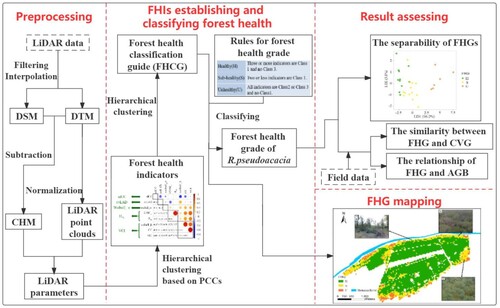
Figure 2 shows an overview of establishing the forest health indicators (FHIs) and classifying forest health in four steps. In the first step, the normalized LiDAR point cloud data were used to construct the canopy height model (CHM), from which the LiDAR parameters were then derived. In the second step, the FHIs were established via hierarchical clustering based on Pearson correlation coefficients (PCCs). Hierarchical clustering was also employed to construct the forest health classification guide (FHCG), which was used to determine the forest health grade (FHG) of R.pseudoacacia. In the third step, the FHG based on FHCG was assessed by field data. The last step is to map the FHG of R.pseudoacacia forest in the Gudao forest.

Figure 2. The workflow for the establishment of the FHIs.

2.3.1. Preprocessing and LiDAR parameters

The LiDAR data were preprocessed in LiDAR 360 3.1 software (Green Valley, Being, China). First, the LiDAR point clouds were denoised to remove outliers. Then, the clouds were filtered into ground points and vegetation points. The digital elevation model (DEM) and digital surface model (DSM) were generated by interpolation of ground points and the maximum number of vegetation points, respectively. The CHM was subsequently constructed by subtracting the DEM from the DSM with a pixel size of 1 m. The LiDAR point clouds were normalized against the DEM.

2.3.1.1. Vertical structure parameters

The vertical structural parameters were extracted from the normalized point clouds. To avoid outliers, the 99th percentile height (H₉₉) was used to represent the maximum tree height at the plot scale (Huesca et al. 2019). The extraction of the other four parameters required vertical stratification of the point clouds.

The canopy height profile (CHP) is represented by the ratio of the number of point clouds in a certain height layer to the total number of point clouds, which describes the vertical distribution of photosynthesis and nonphotosynthetic tissue (Zhao, Popescu, and Nelson 2009). The height percentiles, instead of the height layer, were used to simplify the CHP into 10 height layers in this study. The two-parameter Weibull density function was applied to fit the CHP, and the scale parameter (α) and shape parameter (β) were derived by the maximum likelihood estimation method (Equation (4(4) $\mathrm{f}\left(x\right)=\text{β}/\alpha (x/\alpha {)}^{\text{β}-1}\exp [-{\left(x/\alpha \right)}^{\text{β}}]$(4) )) (Tompalski et al. 2015; Zhang, Lin, and She 2017): (4) $\mathrm{f}\left(x\right)=\text{β}/\alpha (x/\alpha {)}^{\text{β}-1}\exp [-{\left(x/\alpha \right)}^{\text{β}}]$(4) where f(x) is the point cloud density, x is the height percentiles, and α and β refer to the scale and shape parameters of the Weibull density function, respectively.

Leaf area density (LAD) can describe the vertical structure distribution of photosynthetic tissues in forests, and its estimation depends on LAI (Detto et al. 2015). LAI is calculated based on the Beer–Lambert law (Richardson, Moskal, and Kim 2009). When derived from LiDAR data, it was calculated by dividing the gap fraction of the height layers by height Δz. LAD was defined according to the number of point clouds above and below the target height layer i (Detto et al. 2015). The calculation formulae are as follows: (5) $\mathrm{L}\mathrm{A}{\mathrm{D}}_{\mathrm{i}}=-\ln \left(\mathrm{G}{\mathrm{F}}_{\mathrm{i}}\right)/\kappa \mathrm{\Delta }\mathrm{z}$(5) (6) $\mathrm{G}{\mathrm{F}}_{\mathrm{i}}={\mathrm{n}}_{\mathrm{b}\mathrm{e}}/\left(n_{tot}-n_{ab}\right)$(6) where GF is the gap fraction, κ is the extinction coefficient (a value of 0.5 was adopted in this study), n_ab is the number of point clouds above the height layer, n_be is the number of point clouds below the height layer, and n_tot is the number of point clouds. The coefficient of variation (cvLAD) (Equation (7(7) $\mathrm{c}\mathrm{v}\mathrm{L}\mathrm{A}\mathrm{D}=\sqrt{1/H-1\sum _{\mathrm{h}=1}^{\mathrm{H}}{\left(\mathrm{L}\mathrm{A}{\mathrm{D}}_{\mathrm{h}}-\overline{\mathrm{L}\mathrm{A}\mathrm{D}}\right)}^2}/\overline{\mathrm{L}\mathrm{A}\mathrm{D}}$(7) )) (Carrasco et al. 2019) was used to quantify the vertical variation in leaves: (7) $\mathrm{c}\mathrm{v}\mathrm{L}\mathrm{A}\mathrm{D}=\sqrt{1/H-1\sum _{\mathrm{h}=1}^{\mathrm{H}}{\left(\mathrm{L}\mathrm{A}{\mathrm{D}}_{\mathrm{h}}-\overline{\mathrm{L}\mathrm{A}\mathrm{D}}\right)}^2}/\overline{\mathrm{L}\mathrm{A}\mathrm{D}}$(7) where H is the total number of height layers and $\overline{\mathrm{L}\mathrm{A}\mathrm{D}}$ is the mean LAD across all layers.

The vertical complexity index (VCI) (van Ewijk, Treitz, and Scott 2011) was used to quantify the vertical distribution of all aboveground vegetation, and it is calculated as: (8) $\mathrm{V}\mathrm{C}\mathrm{I}=-\sum _{\mathrm{i}=1}^{\mathrm{n}}\left[{\mathrm{P}}_{\mathrm{i}}\ast \mathrm{l}\mathrm{n}\left({\mathrm{P}}_{\mathrm{i}}\right)\right]/\mathrm{l}\mathrm{n}\left(\mathrm{n}\right)$(8) where n represents the total number of elevation levels divided vertically, and P_i represents the portion of points in each elevation level out of the total point cloud (%). A VCI value of one indicates that the canopy configuration is more evenly distributed than that of zero in the vertical direction.

2.3.1.2. Horizontal structure parameters

The horizontal structural parameters are divided into two parts. One part is extracted based on CHM, which is a surface model expressing the height of vegetation from the ground. The standard deviation of CHM (CHM_std) is a continuous parameter that represents vegetation heterogeneity based on canopy heights (Huesca et al. 2019). The other part is extracted based on point cloud. Canopy cover (CC) is defined as the vertical projection area of forest canopies divided by the total stand area, which can reflect the stand density (Lefsky et al. 2002). The horizontal change of canopy cover within a stand can be expressed by the standard deviation of canopy cover (sdCC) (Moran, Rowell, and Seielstad 2018). For a 30 m × 30 m plot, it was first split into 900 subplots of 1 m² each. The sdCC was derived by calculating the CC for each subplot and assigning the standard deviation of the subplot CCs to the plot. The definitions of all LiDAR parameters are summarized in Table 4. All the parameters were calculated by the lidR package and the raster package in R software and extracted with 30 m resolution, which matched the size of field plot.

Table 4. The summary of LiDAR parameters.

	LiDAR parameter	Description	Reference
Vertical structure parameters	H99	The percentiles of the height distributions (99th) of all points above 2 m.	(Huesca et al. 2019)
	Weibull_α	The scale parameter of the Weibull density function fitted to CHP.	(Tompalski et al. 2015)
	Weibull_β	The shape parameter of the Weibull density function fitted to CHP.	(Tompalski et al. 2015)
	cvLAD	The coefficient of variation of leaf area density.	(Carrasco et al. 2019)
	VCI	Vertical complexity index.	(van Ewijk, Treitz, and Scott 2011)
Horizontal structure parameters	CHMstd	The standard deviation of canopy height model with 1 m resolution.	(Huesca et al. 2019)
	CC	Canopy cover (the percentages of first returns above 2 m).	(Lefsky et al. 2002)
	sdCC	Standard deviation of canopy cover.	(Moran, Rowell, and Seielstad 2018)

2.3.2. Establishment of FHIs and FHCG

Cluster analysis is an exploratory classification technique in which samples that are closer together are classified into one category by calculating the distance between them, and those that are farther apart belong to different categories (Kaufman and Rousseeuw 2009; Thompson et al. 2016). Without prior knowledge, that is, training samples, a set of forest health indicators (FHIs) is directly explored and constructed from UAV LiDAR point cloud data by an unsupervised clustering method. The specific steps are as follows. First, the LiDAR parameters with a similar correlation were grouped into one category via hierarchical clustering analysis using the Pearson correlation coefficient (r) as the pairwise distance metric. According to the principle that the correlation coefficient within the category is the largest (representing all indicators of the category) and the correlation coefficient between the categories is the least (having the lowest correlation with indicators of other categories), only one parameter was selected from each category to constitute forest health indicators. Then, each indicator was divided into three classes by hierarchical clustering, corresponding to healthy, subhealthy, and unhealthy forest health grades, and used to established a forest health classification guide (FHCG). The above steps were realized by the corrplot function and hclust function in R software.

2.3.3. Classification and assessment

The FHG of 30 plots was defined according to the rules in Table 5, namely, healthy (H), subhealthy (S), and unhealthy (U). The method of grade determination is to see if a plot meets the healthy or unhealthy criteria. Plots that qualify for neither of these grades are assigned to the subhealthy grade.

Table 5. Rules for determining the FHG based on forest health indicator.

Grade	The number of the indicator classification
Healthy (H)	Three or more indicators are Class 1 and not Class 3.
Subhealthy (S)	Two or less indicators are Class 1.
Unhealthy (U)	All indicators are Class 2 or Class 3 and not Class 1.

The verification of the results was divided into two parts. The first part was the evaluation of classification results. Linear discriminate analysis (LDA) (Li and Yuan 2005) was applied to 30 field plots to visually determine the degree of separation between three FHGs. The nonparametric Kruskal–Wallis test (Breslow 1970) was used to determine differences in FHIs among the three health grades. The second part was to verify the rationality of the FHG, the CVG, and ABG of 30 field plots as test data. To judge whether the FHG based on LiDAR structural parameters can represent forest canopy vigor, the similarity between the FHG and the CVG was calculated by the indicator SIM (Han and Kamber 2007): (9) $\mathrm{S}\mathrm{I}\mathrm{M}={\mathrm{n}}_{\mathrm{s}\mathrm{a}\mathrm{m}\mathrm{e}}/{\mathrm{n}}_{\mathrm{t}\mathrm{o}\mathrm{t}}$(9) where n_same is the number of plots with the same discriminant results and n_tol is the total number of plots. It measures how similar two grades are, with a score of 0–1. Moreover, the relationship between FHG and AGB was measured by the Spearman rank correlation coefficient (r_s) (Spearman 1987) (Equation (10(10) $r_{\mathrm{s}}=1-6\sum _{\mathrm{i}=1}^{\mathrm{n}}{\mathrm{d}}_{\mathrm{i}}^2/\mathrm{n}\left({\mathrm{n}}^2-1\right)$(10) )): (10) $r_{\mathrm{s}}=1-6\sum _{\mathrm{i}=1}^{\mathrm{n}}{\mathrm{d}}_{\mathrm{i}}^2/\mathrm{n}\left({\mathrm{n}}^2-1\right)$(10) where n is the number of plots and d_i is the rank difference of FHG and AGB in each plot. The result can be positive correlation, negative correlation and no correlation. These steps were performed using the MASS package and ggplot2 package in R software.

2.3.4. FHG mapping

In order to generate the FHG map covering the entire study area, the study area was segmented, with a cell size of 30 m × 30 m corresponding to the field plot. Five FHIs were extracted from the cell. According to the FHCG obtained in the previous steps and combined with Table 5, the FHG map can be obtained. Finally, the different degraded forms of R.pseudoacacia were classified with the photos taken by field investigations.

3. Results

3.1. FHIs and FHCG

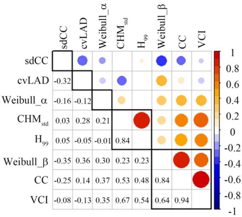
Five categories were grouped from the LiDAR parameters (Figure 3). The first category consisted of Weibull_β, CC, and VCI with a correlation coefficient of 0.64–0.94, and the second category contained CHM_std and H₉₉ (r = 0.84). sdCC, cvLAD, and Weibull_α were each grouped into separate categories (r < 0.5). According to the principle that the selected parameter should have the largest intraclass and the smallest interclass value, the parameters of Weibull_α, H₉₉, and VCI were selected in three categories. Therefore, the FHIs were composed of five parameters, i.e. Weibull_α, H₉₉, VCI, sdCC, and cvLAD.

Figure 3. The correlation matrix heatmap of LiDAR parameters. The circles represent the Pearson correlation coefficient (r) values. The red and blue colors represent the positive and negative values, respectively.

Table 6 and Table 7 showed the established FHCG, in which each indicator was recorded in three classes. Class 1 represents a healthy condition characterized by tall trees (H₉₉), flourishing canopies (Weibull_α, cvLAD), and evenly distributed vegetation both vertically (VCI) and horizontally (sdCC). In contrast, class 3 is unhealthy. The trees are short, and the canopy is not closed. Class 2 does not meet the criteria of either class 1 or 3.

Table 6. Forest health indicators and classification thresholds 1.

Indicator	Class 1	Class 2	Class 3
Weibull_α	>5.57	4.89∼5.57	<4.89
H99	>14.56	11.33∼14.56	<11.33
cvLAD	<0.51	0.51∼0.86	>0.86
VCI	>0.76	0.51∼0.76	<0.51

Table 7. Forest health indicators and classification thresholds 2.

Threshold		Class
VCI	sdCC
>0.76	<0.32	Class 1
	>0.32	Class 2
0.51∼0.76	<0.26	Class 1
	0.26∼0.32	Class 2
	>0.32	Class 3
<0.51	<0.26	Class 2
	>0.26	Class 3

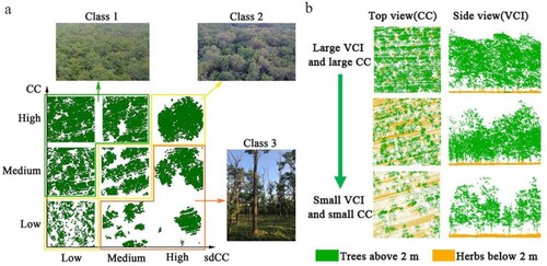
The classification of sdCC (Table 7) is different because it presents different distribution patterns in different CC classes (Figure 4a). Class 1 has a high CC and low sdCC, thereby suggesting the high uniformity of the canopy in the horizontal direction (red box in Figure 4a). The plot with a low CC but a high sdCC (blue box in Figure 4a) indicates that most of the tree canopies have dieback; however, there are trees that are still growing well (Class 3 in Figure 4a). In the FHI establishment step, VCI was selected. VCI and CC are highly correlated (r = 0.94), which can reflect the same stand status (Figure 4b). Therefore, VCI was selected to judge the class of sdCC instead of the CC in this study.

Figure 4. (a) The spatial configuration of canopy cover (CC) and standard deviation of canopy cover (sdCC). The green, yellow and orange boxes correspond to the three classes of sdCC. The pictures named Class 1, Class 2 and Class 3 were taken in the field. (b) The relationship between VCI and CC from two views.

3.2. Assessment on separability and similarity

The LDA on 30 field plots indicated that the FHGs can be separated explicitly in the two discriminate coefficient axes, except for one healthy and subhealthy plot that had a partial overlap (Figure 5a). The Kruskal–Wallis test result showed that all the selected indicators except cvLAD (p = 0.087) were significantly different (p < 0.05) among the three FHGs (Table 8). However, if the insignificant indicator cvLAD was removed, there was more overlap between healthy and subhealthy plots by using the remaining four indicators (Figure 5b).

Figure 5. The FHGs of R.pseudoacacia forest plotted against two discriminant axes. The FHGs were produced by using (a) all FHIs and (b) only four significant indicators, i.e. Weibull_α, H_99, VCI, and sdCC.

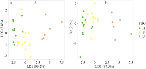
Table 8. Kruskal-Wallis test p values by FHIs.

Indicator	p value
weibull_α	<0.001
H99	0.010
cvLAD	0.087
VCI	<0.001
sdCC	<0.001

The calculated SIM value between the FHG and the CVG was 63.33%, indicating that the majority of the FHG had the same grade as the CVG. Moreover, the FHG was significantly correlated with the forest AGB (r_s = 0.51, p = 0.004), while CVG was not (r_s = 0.097, p = 0.61).

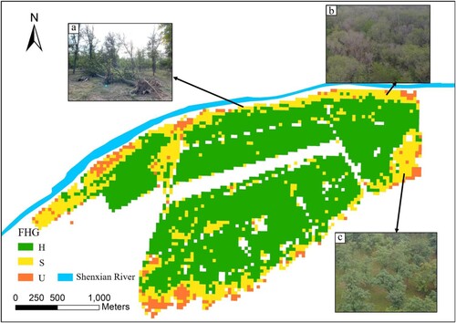
3.3. FHG map

Figure 6 is the FHG map covering the entire study area generated based on FHIs. Based on field surveys, the degraded R.pseudoacacia trees were distributed on the north and south sides of the study area, while trees growing in the middle are in good health. Windthrow (Figure 6a) and trees with severe canopy dieback (Figure 6b) were distributed along the river in the north. The trees in the south of the study area grew short and had large gaps between trees, but the leaves are green and without defoliation (Figure 6c).

Figure 6. FHG map and degradation of R.pseudoacacia in Gudao forest. (a) The windthrow caused by cyclonic storms. (b) The stand with severe dieback. (c) The stand with short trees and low canopy cover but low canopy dieback.

4. Discussion

4.1. Contribution and variability of FHIs

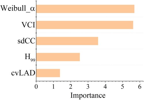
In order to explore the role of each indicator in forest health assessment, we used LDA to evaluate it from the modeling perspective, which was estimated by comparing the performance of all LDA models, removing one indicator each time. The result indicated that Weibull_α and VCI were the most important indicators, followed by sdCC and H₉₉, and cvLAD was relatively less important (Figure 7).

Figure 7. The importance rank of FHI based on LDA.

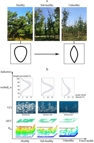
With the degradation of R.pseudoacacia, the shape of the canopy changed from obovate to spindle (Figure 8a); thus, the indicators reflecting the canopy three-dimensional structure changed obviously. Figure 8b shows the structural and morphological variability of the four indicators with the largest contribution in Figure 7 under different FHGs. The indicator Weibull_α was a good indicator of canopy shape with a higher value and a higher peak point (the percentile height of H₆₅) on the fitting curve at a healthy plot and a smaller value and a lower peak point (the percentile height of H₃₀) at an unhealthy plot (the first row of Figure 8b). The VCI described the vertical distribution of tree components such as leaves and branches. With the decline in tree health status, the point clouds were concentrated in the lower canopy and understory layers with a declining VCI value (the second row of Figure 8b). The trees in healthy plots were generally higher (the third row of Figure 8b). From the top view, indicator sdCC described the canopy horizontal distribution. In the healthy plots, the trees flourished with a large VCI, and the sdCC was small (the fourth row of Figure 8b), thereby indicating closed forest and little variability.

Figure 8. (a) R.pseudoacacia in different FHGs and the corresponding shape of the canopy vertical section. (b) The structural and morphological differences of indicators in three different FHGs.

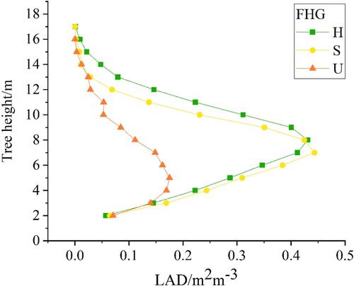
The cvLAD with poor contribution was less separable among three health grades than the other four FHIs. This is because the R.pseudoacacia plantation in the study area had a single stand and only grass with different degrees of light loving under the stand (Wang, Lu, and Pu 2016), resulting in a peak in the middle of the LAD profile in all three health status stands (Figure 9). The cvLAD is a minor indicator, however, it can be significant in specific cases, especially at the deciduous stands (Bouvier et al. 2015). At the same time, our result also showed that discrimination confusion would increase when this indicator was refused (Figure 5). Therefore, cvLAD was still included by FHIs. In our study, the distinction between healthy and unhealthy stands was confused because their canopy shape and stand structure were similar. Compared with the flourishing crowns in healthy stands, the subhealthy trees only had slight defoliation in the treetops and some lateral branches. As in previous studies, there was no clear boundary between the two (Wang et al. 2015). Better indicators and methods to accurately distinguish the subhealthy are our future work.

Figure 9. Vertical profiles of LAD plotted according to the mean values of LAD of the plots at different health grades.

4.2. FHIs vs CVIs

Because of the low terrain, the groundwater level in the study area is generally lower than 1.5 m, resulting in the widespread distribution of saline soil (Chen et al. 2019; Wu, Liu, and Huang 2016). The R.pseudoacacia forests have been in the later stage of degradation due to the long-term adverse water and salt conditions. To understand the difference between FHIs and CVIs, correlation analysis was performed. Table 9 showed that Weibull_ α and VCI were highly correlated with CVIs, which played an important role in identifying the dieback stand. For example, in the north part of the study area (Figure 6b), the trees have serious dieback and low canopy density. The low correlation with CVIs was the vertical structure indicator (H₉₉ and cvLAD) (Table 9), which is the advantage of FHI. Compared with CVIs reflecting canopy appearance, the structural parameters extracted from LiDAR can provide more detailed 3D structural heterogeneity information for forest health assessment (Bourgoin et al. 2020) and are more suitable for forests with obvious structural differentiation in late degradation. For example, in the southern part of the study area (Figure 6c), the growth of trees has been inhibited since planting with small height and DBH values due to long term and slow disturbance (Lu et al. 2020), so the trees are not healthy. Since there was no tree crown dieback, the tree was considered as healthy when discriminating by CVI, because only the indicator of crown diameter was in Class 2, and the other four indicators were in Class 1. However, when using FHI, the grade was corrected to subhealthy or even unhealthy because of the unqualified H₉₉, sdCC and cvLAD. Therefore, the advantage of FHIs is that the horizontal indicators play the same role as CVIs in characterizing tree canopy vigor, while the vertical indicators compensate for the deficiency in characterizing tree productivity.

Table 9. The Pearson correlation coefficient of FHIs and CVIs.

	Weibull_α	H99	cvLAD	VCI	sdCC
Live crown ratio	0.79	0.01	0.30	0.63	−0.34
Crown diameter	0.64	0.12	0.23	0.76	−0.45
Crown density	0.75	0.09	0.17	0.88	−0.57
Crown dieback	−0.82	0.05	0.28	−0.75	0.38
Foliar transparency	−0.68	0.02	0.34	−0.80	0.52

At the early stage of disturbance, leaf biochemical parameters such as chlorophyll and water content changed. However, LiDAR-based indictors lose effectiveness when the leaves are discolored but not dropped (Torres et al. 2021). At this time, optical and hyperspectral remote sensing image data can play a role (Huang, Anderegg, and Asner 2019). Therefore, the combination of LiDAR data and hyperspectral remote sensing imagery will be the future direction of forest health status identification and quantification, which can monitor the stage or degree of forest degradation to take corresponding management countermeasures. In addition, due to the disadvantages of expensive data acquisition and limited coverage area of LiDAR, canopy texture analysis based on very high spatial resolution (VHSR) optical imagery also provides an alternative indicator for forest structure assessment (Bourgoin et al. 2020; Dash et al. 2017). In the future, the correlation between canopy texture extracted from VHSR optical imagery with continuous coverage and forest structural parameters extracted from LiDAR covering local typical areas can be used to complete rapid assessment of forest health on a large scale.

5. Conclusions

In this study, a new set of FHIs was established by using UAV-LiDAR data and cluster analysis, which demonstrated the potential of LiDAR technology in forest health monitoring. The results showed that the FHIs, including Weibull_α, VCI, sdCC, H₉₉, and cvLAD, could clearly distinguish forest health status without prior classification information. The LDA identified Weibull_α and VCI as the dominant indicators, but the comprehensive use of five indicators can improve the accuracy of health status discrimination. FHIs could consider both canopy vigor and tree productivity when evaluating forest health, with a similarity between the FHG and the CVG of 63.33% and a significant positive correlation (r_s = 0.51, p = 0.004) with the forest AGB. With the decline of R.pseudoacacia health status, the canopy spatial structure changed: the shape of the canopy changed from obovate to spindle (Weibull_ α), the situation of canopy dieback intensified (cvLAD), and the structural variability of the vertical and horizontal directions increased (VCI, sdCC). In addition, the unhealthy R.pseudoacacia was generally shorter (H₉₉). FHIs can be easily obtained from LiDAR data, and the development and popularity of LiDAR technology enables rapid and effective monitoring of forest health with no or few field plots.

Data availability statement

The data that support the findings of this study are openly available in ‘Zenodo’ at https://doi.org/10.5281/zenodo.5724611.

Disclosure statement

No potential conflict of interest was reported by the author(s).

Additional information

Funding

This work was supported by National Natural Science Foundation of China: [Grant Number No. 41471419 and No. 31971579].

References

- Arnott, J. C., E. C. Osenga, J. L. Cundiff, and J. W. Katzenberger. 2015. “Engaging Stakeholders on Forest Health: A Model for Integrating Climatic, Ecological, and Societal Indicators at the Watershed Scale.” Journal of Forestry 113: 447–453.
- Asner, G. P., D. Nepstad, G. Cardinot, and D. Ray. 2004. “Drought Stress and Carbon Uptake in an Amazon Forest Measured with Spaceborne Imaging Spectroscopy.” Proceedings of the National Academy of Sciences of the United States of America 101: 6039–6044.
- Bourgoin, C., J. Betbeder, P. Couteron, L. Blanc, H. Dessard, J. Oszwald, R. Le Roux, et al. 2020. “UAV-based Canopy Textures Assess Changes in Forest Structure from Long-Term Degradation.” Ecological Indicators 115: 106386.
- Bouvier, M., S. Durrieu, R. A. Fournier, and J. Renaud. 2015. “Generalizing Predictive Models of Forest Inventory Attributes Using an Area-Based Approach with Airborne LiDAR Data.” Remote Sensing of Environment 156: 322–334.
- Breslow, Norman. 1970. “A Generalized KRUSKAL-WALLIS Test for Comparing K Samples Subject to Unequal Patterns of Censorship.” Biometrika 57: 579–594.
- Bussotti, F., and M. Pollastrini. 2017. “Traditional and Novel Indicators of Climate Change Impacts on European Forest Trees.” Forests 8: 137.
- Cammarano, D., F. Glenn, B. Bruno, O. Garry, and F. Costanza. 2015. “Use of the Canopy Chlorophyl Content Index (CCCI) for Remote Estimation of Wheat Nitrogen Content in Rainfed Environments.” Agronomy Journal 103: 1597–1603.
- Carrasco, L., X. Giam, M. Papeş, and K. Sheldon. 2019. “Metrics of Lidar-Derived 3D Vegetation Structure Reveal Contrasting Effects of Horizontal and Vertical Forest Heterogeneity on Bird Species Richness.” Remote Sensing 11: 743.
- Chen, X., and D. G. Brockway. 2017. “Height-diameter Relationships in Longleaf Pine and Four Swamp Tree Species.” Journal of Plant Studies 6: 94–101.
- Chen, H., G. Zhao, Y. Li, D. Wang, and Y. Ma. 2019. “Monitoring the Seasonal Dynamics of Soil Salinization in the Yellow River Delta of China Using Landsat Data.” Natural Hazards and Earth System Sciences 19: 1499–1508.
- Cherubini, P., G. Battipaglia, and J. L. Innes. 2021. “Tree Vitality and Forest Health: Can Tree-Ring Stable Isotopes Be Used as Indicators?” Current Forestry Reports 7: 69–80.
- Coops, N. C., A. Varhola, C. W. Bater, P. Teti, S. Boon, and N. M. Weiler. 2009. “Assessing Differences in Tree and Stand Structure Following Beetle Infestation Using Lidar Data.” Canadian Journal of Remote Sensing 35: 497–508.
- Dash, J. P., M. S. Watt, G. D. Pearse, M. Heaphy, and H. S. Dungey. 2017. “Assessing Very High Resolution UAV Imagery for Monitoring Forest Health During a Simulated Disease Outbreak.” Isprs Journal of Photogrammetry and Remote Sensing 131: 1–14.
- Detto, M., G. P. Asner, H. C. Muller-Landau, and O. Sonnentag. 2015. “Spatial Variability in Tropical Forest Leaf Area Density from Multireturn Lidar and Modeling.” Journal of Geophysical Research Biogeosciences 120: 294–309.
- Eitel, J. U. H., L. A. Vierling, M. E. Litvak, D. S. Long, U. Schulthess, A. A. Ager, D. J. Krofcheck, and L. Stoscheck. 2011. “Broadband, red-Edge Information from Satellites Improves Early Stress Detection in a New Mexico Conifer Woodland.” Remote Sensing of Environment 115: 3640–3646.
- FAO. 2020. Global Forest Resources Assessment 2020. Rome, Italy: Food and Agriculture Organization of the United Nations.
- Gao, T., M. Hedblom, T. Emilsson, and A. B. Nielsen. 2014. “The Role of Forest Stand Structure as Biodiversity Indicator.” Forest Ecology and Management 330: 82–93.
- Grulke, N., C. Bienz, K. Hrinkevich, J. Maxfield, and K. Uyeda. 2020. “Quantitative and Qualitative Approaches to Assess Tree Vigor and Stand Health in dry Pine Forests.” Forest Ecology and Management 465: 118085.
- Han, J., and M. Kamber. 2007. Data Mining: Concepts and Techniques. Beijing: China Machine Press.
- Hansen, M. C., P. V. Potapov, R. Moore, M. Hancher, S. A. Turubanova, A. Tyukavina, and D. Thau. 2013. “High-Resolution Global Maps of 21st-Century Forest Cover Change.” Science 342: 850–853.
- Huang, C., W. R. L. Anderegg, and G. P. Asner. 2019. “Remote Sensing of Forest die-off in the Anthropocene: From Plant Ecophysiology to Canopy Structure.” Remote Sensing of Environment 231: 111233.
- Huesca, M., K. L. Roth, M. García, and S. L. Ustin. 2019. “Discrimination of Canopy Structural Types in the Sierra Nevada Mountains in Central California.” Remote Sensing 11: 1100.
- Jiang, F., J. Zhu, and D. Zeng. 2003. Management for Protective Plantations. Beijing: China Forestry Publishing.
- Kaufman, L., and P. J. Rousseeuw. 2009. Finding Groups in Data: An Introduction to Cluster Analysis.
- Kramer, H. 1966. “Crown Development in Conifer Stands in Scotland as Influenced by Initial Spacing and Subsequent Thinning Treatment.” Forestry 39: 40–58.
- Lausch, A., S. Erasmi, D. King, P. Magdon, and M. Heurich. 2016. “Understanding Forest Health with Remote Sensing -Part I—A Review of Spectral Traits, Processes and Remote-Sensing Characteristics.” Remote Sensing 8: 1029.
- Lausch, A., S. Erasmi, D. King, P. Magdon, and M. Heurich. 2017. “Understanding Forest Health with Remote Sensing-Part II—A Review of Approaches and Data Models.” Remote Sensing 9: 129.
- Leeuwen, M. V., and M. Nieuwenhuis. 2010. “Retrieval of Forest Structural Parameters Using LiDAR Remote Sensing.” European Journal of Forest Research 129: 749–770.
- Lefsky, M. A., W. B. Cohen, G. G. Parker, and D. J. Harding. 2002. “Lidar Remote Sensing for Ecosystem Studies.” Bioscience 52: 19.
- Li, M., and B. Yuan. 2005. “2D-LDA: A Statistical Linear Discriminant Analysis for Image Matrix.” Pattern Recognition Letters 26: 527–532.
- Lu, J., H. Wang, S. Qin, L. Cao, R. Pu, G. Li, and J. Sun. 2020. “Estimation of Aboveground Biomass of Robinia Pseudoacacia Forest in the Yellow River Delta Based on UAV and Backpack LiDAR Point Clouds.” International Journal of Applied Earth Observation and Geoinformation 86: 102014.
- Marco, F. 1997. “Forest Health Assessment and Monitoring – Issues for Consideration.” Environmental Monitoring and Assessment 48: 45–72.
- Moran, C. J., E. M. Rowell, and C. A. Seielstad. 2018. “A Data-Driven Framework to Identify and Compare Forest Structure Classes Using LiDAR.” Remote Sensing of Environment 211: 154–166.
- Næsset, E. 2002. “Predicting Forest Stand Characteristics with Airborne Scanning Laser Using a Practical two-Stage Procedure and Field Data.” Remote Sensing of Environment 80: 88–99.
- Næsset, E., and T. Gobakken. 2008. “Estimation of Above- and Below-Ground Biomass Across Regions of the Boreal Forest Zone Using Airborne Laser.” Remote Sensing of Environment 112: 3079–3090.
- Pan, Y., R. A. Birdsey, J. Fang, R. Houghton, P. E. Kauppi, W. A. Kurz, O. L. Phillips, et al. 2011. “A Large and Persistent Carbon Sink in the World's Forests.” Science 333: 988–993.
- Pause, M., C. Schweitzer, M. Rosenthal, V. Keuck, J. Bumberger, P. Dietrich, M. Heurich, A. Jung, and A. Lausch. 2016. “In Situ/Remote Sensing Integration to Assess Forest Health—A Review.” Remote Sensing 8: 471.
- Potter, K. M., and B. L. Conkling. 2016. Forest health monitoring:national status, trends, and analysis 2015 199 pp.
- Richardson, J. J., L. M. Moskal, and S. Kim. 2009. “Modeling Approaches to Estimate Effective Leaf Area Index from Aerial Discrete-Return LIDAR.” Agricultural and Forest Meteorology 149: 1152–1160.
- Schomaker, M. E., S. J. Zarnoch, W. A. Bechtold, D. J. Latelle, and W. G. Burkman. 2007. “Crown-condition classification: a guide to data collection and analysis”.
- Silva, C. A., C. Klauberg, A. T. Hudak, L. A. Vierling, V. Liesenberg, and S. P. C. E. Carvalho. 2016. “A Principal Component Approach for Predicting the Stem Volume in Eucalyptus Plantations in Brazil Using Airborne LiDAR Data.” Forestry 89 (4): 422–433.
- Smigaj, M., R. Gaulton, J. C. Suárez, and S. L. Barr. 2019. “Combined use of Spectral and Structural Characteristics for Improved red Band Needle Blight Detection in Pine Plantation Stands.” Forest Ecology and Management 434: 213–223.
- Spearman, C. 1987. “The Proof and Measurement of Association Between two Things. By C. Spearman, 1904.” American Journal of Psychology 100: 441–471.
- Thompson, S. D., T. A. Nelson, I. Giesbrecht, G. Frazer, and S. C. Saunders. 2016. “Data-driven Regionalization of Forested and non-Forested Ecosystems in Coastal British Columbia with LiDAR and RapidEye Imagery.” Applied Geography 69: 35–50.
- Tompalski, P., N. Coops, J. White, and M. Wulder. 2015. “Enriching ALS-Derived Area-Based Estimates of Volume Through Tree-Level Downscaling.” Forests 6: 2608–2630.
- Torres, P., M. Rodes-Blanco, A. Viana-Soto, H. Nieto, and M. García. 2021. “The Role of Remote Sensing for the Assessment and Monitoring of Forest Health: A Systematic Evidence Synthesis.” Forests 12: 1134.
- Trumbore, S., P. Brando, and H. Hartmann. 2015. “Forest Health and Global Change.” Science 349: 814–818.
- van Ewijk, K. Y., P. M. Treitz, and N. A. Scott. 2011. “Characterizing Forest Succession in Central Ontario Using Lidar-Derived Indices.” Photogrammetric Engineering & Remote Sensing 77: 261–269.
- Wang, H., K. Lu, and R. Pu. 2016. “Mapping Robinia Pseudoacacia Forest Health in the Yellow River Delta by Using High-Resolution IKONOS Imagery and Object-Based Image Analysis.” Journal of Applied Remote Sensing 10: 045022.
- Wang, H., R. Pu, Q. Zhu, L. Ren, and Z. Zhang. 2015. “Mapping Health Levels of Robinia Pseudoacacia Forests in the Yellow River Delta, China, Using IKONOS and Landsat 8 OLI Imagery.” International Journal of Remote Sensing 36: 1114–1135.
- Woodall, C. W., M. C. Amacher, W. A. Bechtold, J. W. Coulston, S. Jovan, C. H. Perry, K. C. Randolph, et al. 2011. “Status and Future of the Forest Health Indicators Program of the USA.” Environmental Monitoring and Assessment 177: 419–436.
- Wu, C., G. Liu, and C. Huang. 2016. “Prediction of Soil Salinity in the Yellow River Delta Using Geographically Weighted Regression.” Archives of Agronomy and Soil Science 63: 928–941.
- Zarnoch, S. J., W. A. Bechtold, and K. W. Stolte. 2004. “Using Crown Condition Variables as Indicators of Forest Health.” Canadian Journal of Forest Research 34: 1057–1070.
- Zhang, Z., C. Lin, and G. She. 2017. “Estimating Forest Structural Parameters Using Canopy Metrics Derived from Airborne LiDAR Data in Subtropical Forests.” Remote Sensing 9: 940.
- Zhao, K., S. Popescu, and R. Nelson. 2009. “Lidar Remote Sensing of Forest Biomass: A Scale-Invariant Estimation Approach Using Airborne Lasers.” Remote Sensing of Environment 113: 182–196.
- Zhu, J., D. Zeng, H. Kang, X. Wu, and Z. Fan. 2005. Decline of pinus sylvestris var. mongolica plantations on sandy land. China Forestry Publishing. Beijing 264 pp.