Bathymetric mapping and estimation of water storage in a shallow lake using a remote sensing inversion method based on machine learning

ABSTRACT

Accurate lake depth mapping and estimation of changes in water level and water storage are fundamental significance for understanding the lake water resources on the Tibetan Plateau. In this study, combined with satellite images and bathymetric data, we comprehensively evaluate the accuracy of a multi-factor combined linear regression model (MLR) and machine learning models, create a depth distribution map and compare it with the spatial interpolation, and estimate the change of water level and water storage based on the inverted depth. The results indicated that the precision of the random forest (RF) was the highest with a coefficient of determination (R²) value (0.9311) and mean absolute error (MAE) values (1.13 m) in the test dataset and had high reliability in the overall depth distribution. The water level increased by 9.36 m at a rate of 0.47 m/y, and the water storage increased by 1.811 km³ from 1998 to 2018 based on inversion depth. The water level change was consistent with that of the Shuttle Radar Topography Mission (SRTM) method. Our work shows that this method may be employed to study the water depth distribution and its changes by combining with bathymetric data and satellite imagery in shallow lakes.

KEYWORDS:

• Remote sensing inversion
• lake bathymetry
• Sentinel-2
• machine learning (ML)
• random forest (RF)
• water storage

1. Introduction

The Tibetan Plateau (TP) contains the richest water resources with a large number of lakes that are important information carriers that reveal global climate change and are also extremely sensitive to regional and global climate fluctuations (Jiang et al. 2020). It is of great significance to realize high-precision water depth mapping and estimate the change in the water level and water storage of lakes for regional water cycles (Yang et al. 2014). At present, the overall water depth distribution of lakes is mainly simulated by the spatial interpolation method based on points or tracks that can be obtained from satellite altimetry data or in field survey measurements using depth gauges mounted on boats (Qiao et al. 2017; Yang et al. 2020). This method is time-consuming, labour intensive, and expensive in the field and produces some indefinite factors that affect the accuracy in further processing (Wechsler 2007; Becker et al. 2009; Costa, Battista, and Pittman 2009), and it is a lack of discussion on the accuracy of spatial interpolation where there is no measured depth value distribution. Studies of the changes in water level and storage are mainly estimated by a digital elevation model (DEM) or satellite altimetry data (ICESat, etc.) combined with remote sensing images (Phan, Lindenbergh, and Menenti 2012; Song, Huang, and Ke 2013, 2014; Zhang et al. 2013; Li et al. 2014). Affected by the quantity and location distribution of bathymetric data and the resolution of altimetry data, it is always important to obtain the high-precision water depth of each pixel to estimate water level and storage. Remote sensing (RS) serves a key role in hydroinformatics (Mynett and Vojinovic 2009), and the ability to derive lake bathymetry using RS techniques has been the subject of intense scholarly study; in particular, RS inversion, as a method to obtain water depth distribution, is a low-cost, fast, reliable and prevalent method for estimating shallow water depth (Eugenio, Marcello, and Martin 2015; Caballero and Stumpf 2019).

RS water depth inversion obtains the regional depth distribution by establishing the relationship between water depth (it is generally considered that the water depth needs to be less than 30 m) and image reflectivity, and highly accurate water depth inversion and mapping have become important research directions for remote sensing image applications. Previous researchers have developed many methods based on bathymetry data in the field and remote sensing images (Kutser et al. 2020; Li et al. 2021), mainly including statistical models, theoretical models, and semitheoretical and semiempirical models (Brando et al. 2009; Roy et al. 2014; Hedley et al. 2016; Chénier, Faucher, and Ahola 2018). The statistical model is widely used in remote sensing inversion water depth studies (Liu 2013). The parametric regression model and a nonparametric regression model are two forms of the statistical model. Since the water environment is heterogeneous and complex, traditional parametric statistical models, such as the band ratio model (Stumpf) proposed by Stumpf et al., multiband linear model (Lyzenga) proposed by Lyzenga et al., improved Stumpf model (log-linear relationships), and multiple linear regression, may not be correctly modelled (Lyzenga 1978; Stumpf, Holderied, and Sinclair 2003; Su, Liu, and Heyman 2008); therefore, the nonparametric models using machine learning (ML) have good application prospects in remote sensing water depth inversion. Some researchers have attempted to apply ML approaches that were found to be more accurate for relating remote sensing images to bathymetry data to improve retrieval precision in recent years. Wan and Ma (2021) documented a deep belief network with a data perturbation (DBN-DP) algorithm based on a back-propagation neural network (BP) structure for nearshore bathymetry from a high-resolution multispectral image of Xinji Island, which showed 12.8% MRE and 1.2 m MAE. Mateo-Pérez et al. (2020) used the support vector machine (SVM) model and Sentinel-2 images to experiment in two different ports that are highly polluted, turbid and have depths less than 12 m. The results showed that the RMSE was less than 0.5 m. Yunus et al. (2019) compared an empirical approach and a random forest (RF) model based on Sentinel-2 and Landsat-8 images, the RF model with an RMSE between 1.13 and 1.95 m demonstrated that the RF model is suitable and effective in coastal and lake environments. At the top of the highest hierarchy are ML water depth inversion algorithms, which use self-adaptation, self-learning, and self-organization, especially nonlinear dynamic processing, which can provide more precise results than traditional statistical models (Sandidge and Holyer 1998; Mas and Flores 2008; Liu et al. 2018).

To the best of our knowledge, in remote sensing water depth inversion, past studies mainly compared various traditional statistical regression models or examined the ability of a single machine learning model, study sites were mainly located on islands, ports, reservoirs, estuaries, and coastal areas because they had relatively spatially extensive, sediment uniform (Hodúl et al. 2018). There have been no detailed studies comparing the accuracy of BP, SVM and RF models in lake water depth inversion under the same experimental conditions in inland shallow lake. In particular, on the TP, many shallow lakes are located in extreme locations, bathymetry requires considerable manpower and material resources. In addition, in the study of the change of lake level and storage, there have been no studies on estimating water level, water storage, and its change based on remote sensing inversion depth.

In this study, based on Sentinel-2 satellite imagery data and bathymetry data of QiXiang Co on the TP, we proposed to combine the classical band reflectance logarithm and logarithm ratio factor to construct a multi-factor combined linear regression (MLR) model and three common machine learning models (BP, SVM and RF), comprehensively compared the performance of them, analyzed the effect of inversion mapping of each model. Importantly, the depth of the bathymetric inversion method and spatial interpolation method was compared in places where there was no measured value. Combined with the boundary data from 1998 to 2018, we also assessed the accuracy of the change of water level and water storage obtained from the remote sensing inversion method, DEM method, and spatial interpolation method, which can be used to provide dependable-precision, high-speed and low-cost data for later use in numerical models in lake research and provide a reference in studying remote sensing depth retrieval and estimating water storage in shallow lakes.

This paper is organized as follows. The next section introduces the type and preprocessing of the data used in this study. Section 3 describes the methods in detail, including the model used in remote sensing depth inversion, the method of model accuracy evaluation and the method of water change estimation. Section 4 presents the results of the model inversion accuracy, provides the water depth distribution map and estimates the water storage and its change based on the inversion results. The effect of segmented depth inversion and model defects are discussed in Section 5. Finally, the conclusion and future improvements are elaborated in Section 6.

2. Data and preprocessing

2.1. Study sites

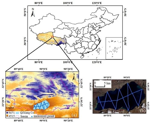
QiXiang Co, as shown in Figure 1, is located in the northwestern of Naqu County on the Tibetan Plateau, which is located in the Shuanghu special area at 32°11′-32°41′N and 89°38′-90°17′ E. It is located in the lake basin belt of the Qiangtang Plateau, with flat mountains and open grasslands. The terrain is high in the north and low in the south, containing mostly arid and semidesert grassland, with an average altitude of 4800 m. There are many lakes, among which QiXiang Co is one. This lake is elliptical in surface distribution, with its axis oriented northeast-southwest and with a maximum width of approximately 20 km. The annual average area and depth of the lake are approximately 180 km² and 14 m, respectively. It enters the freezing period in late November and thaws in early April of the following year. Since there is only one lake in the basin and it is far from the glacier, the water supply is mainly from precipitation.

Figure 1. The location of the study area on the Tibetan Plateau and the measured points. (a) Topographic map. (b) The measured points of QiXiang Co.

2.2. Bathymetry data

Bathymetric data were surveyed in situ in July 2019 using a Lowrance HDS5 bathymetric device installed on a ship and has a vertical accuracy of 0.01 m. The data were recorded once per second, and every measurement point had a corresponding longitude and latitude. The measured route on the QiXiang Co is shown in Figure 1. Affected by the ship’s draft and its environment, the total number of measured points was 16557, which covered the main region, with 0.97 m being the shallowest bathymetric point and 27.60 m being the deepest. Since the ML model is used to invert the water depth, the number of measured sample points largely influences the accuracy of the model training and testing datasets. There may be multiple points in a Sentinel-2 image pixel, and a fishing net with a size of 10 m × 10 m must be established using ArcGIS 10.5 to obtain an average value as the water depth characteristic value is obtained as the experimental data. A total number of 9775 was obtained, as shown in Table 1. When training the model, we set the training dataset to randomly account for 75% of all data.

Table 1. Detailed information on the bathymetry data in QiXiang Co.

Name	Measured plots	Characterization plots	Max depth (m)	Min depth (m)	Mean depth (m)	Training dataset	Testing dataset
QiXiang Co	16557	9775	27.60	0.97	13.96	7332	2443

2.3. Satellite imagery data

Sentinel-2 was launched in June 2015 from French Guiana, designed by Airbus Defence and Space for the European Space Agency (ESA), and is a high-resolution multispectral imaging satellite carrying a Multispectral Imager (MSI) from a height of 786 km (European Space Agency 2021a, 2021b). This sensor has 13 bands from visible to shortwave infrared with resolutions of 10, 20, and 60 m. The revisit period of one satellite is 10 days and that of two complementary satellites (Sentinel-2A/B) is 5 days. The Sentinel-2 images were obtained from the United States Geological Survey (https://earthexplorer.usgs.gov/). To obtain a reliable correlation relationship between the reflectance of the band and measured water depth, images close to the measured data time from July to October in 2018, 2019, and 2020 were obtained on the premise that there were no clouds over the lake. We preliminarily analysed the correlation between the reflectance of the b1, b2, b3, and b4 bands and the measured water depth. Finally, an image on 9 July 2018, with the best correlation (as shown in Table 2) was selected and used in the experiment.

Table 2. The correlation coefficient of different bands and water depths.

Band	Correlation coefficient (R)	Band	Correlation coefficient (R)	Band ratio	Correlation coefficient (R)
b1	−0.7630	lnb1	−0.7722	lnb1/lnb2	0.7134
b2	−0.7791	lnb2	−0.7856	lnb1/lnb3	0.8239
b3	−0.8047	lnb3	−0.8178	lnb1/lnb4	0.8105
b4	−0.7469	lnb4	−0.8021	lnb2/lnb1	−0.7130
b5	−0.0816			lnb2/lnb3	0.8408
b6	−0.1054			lnb2/lnb4	0.7855
b7	−0.0474			lnb3/lnb1	−0.8232
b8	−0.4492			lnb3/lnb2	−0.8402
b8a	−0.1241			lnb3/lnb4	0.6942
b9	−0.3650			lnb4/lnb1	−0.6917
b10	−0.4755			lnb4/lnb2	−0.7795
b11	−0.0567			lnb4/lnb3	−0.8055
b12	−0.0435

Due to the late launch of the Sentinel-2 satellite, this paper also needed to obtain the area boundary data of QiXiang Co from 1998 to 2018 based on Landsat images utilizing the Google Earth Engine (GEE). In addition, we also used used Shuttle Radar Topography Mission (SRTM) in 2000 data (30 m resolution). Sen2cor was used for radiometric calibration and atmospheric correction of the Sentinel-2 image, and ESA snap software was used to resample the image at a 10 m resolution. The image mosaic was completed in ArcGIS10.5, and the coordinate system was converted to a WGS-84 geographic coordinate system. The correlation coefficient (R) between the reflectivity of each band and the measured water depth value is shown in Table 2. We noticed that the bands with a high correlation with water depth were b1, b2, b3, and b4, and logarithmic change could improve the correlation. According to the numerical grade of R (|R|≥0.8 high correlation, 0.5<|R|<0.8 moderate correlation, 0.3<|R|<0.5 low correlation, and |R|<0.3 correlation is very weak), b1, b2, b3, and b4 were selected for the experiment, further considering that the linear model proposed by Lyzenga, as shown in Equation (1), could avoid the influence of the distinctive in sediments (Lyzenga 1985). Therefore, the R values between the logarithm of reflectance in the four bands and the measured water depth values were calculated first. Stumpf proposed a ratio model, as shown in Equation (2), which has a deeper range, better stability, and robustness (Stumpf, Holderied, and Sinclair 2003; Dierssen et al. 2013). We analysed the R between the logarithm ratio of reflectance in four bands and the measured depth value (see Table 2), and four band ratio factors were also selected. Finally, we utilized eight factors, lnb1, lnb2, lnb3, lnb4, lnb1/lnb2, lnb1/lnb3, lnb2/lnb3, and lnb4/lnb3, with strong correlations as modelling factors. (1) $h={\alpha }_0+{\alpha }_i\sum _{i=1}^n\ln [L({\lambda }_i)-L_{\mathrm{\infty }}({\lambda }_i)].$(1) (2) $h={\alpha }_0+{\alpha }_1{\displaystyle \frac{\ln (nL({\lambda }_i))}{\ln (nL({\lambda }_j))}.}$(2) where $h$ is the water depth, ${\alpha }_i$ and ${\alpha }_0$ represent coefficients, $n$ is a fixed constant whose role is to ensure that the ratio is positive and $L({\lambda }_i)$, and $L({\lambda }_j)$ is the reflectance of the ith and jth bands, respectively.

3. Methodology

In remote sensing water depth inversion, the choice of model directly affects the inversion accuracy. Especially with little research on the remote sensing water depth inversion of lakes on the TP, the applicable models needed to be examined. In this research, didferent models were compared, and a relatively optimal model was obtained for further study the change of water depth and water storage. All models were implemented using scikit-learn Library in Python 3.8. Scikit-learn Library had integrated and implemented many mainstream machine learning algorithms, including BP, SVM, RF and so on.

3.1. Back propagation neural network model

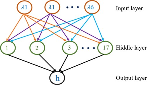
Neural networks utilize intelligent computation combining a computer network system to replicate the biological neural network, which performs a famous superiority in solving large-scale computing and nonlinear problems. It is a very mature network and has been widely used in many research fields (Khoshnevisan, Rafiee, and Omid 2013) and has strong nonlinear mapping ability. The BP named the forward spread of the data stream and the reverse spread of the error signal is a multilayer feedforward network, and it consists of an input layer, hidden layers, and output layer (Mukherjee et al. 2020). The layers are connected by weights, and each layer is composed of neurons. The neurons in each layer can only affect the neurons in the next layer; therefore, when the signal propagates forward, the signal from the input layer to the output layer propagates through the layer-by-layer calculation of the hidden layer. In contrast, when the signal propagates back, the error is calculated as the signal from the output layer through the hidden layer by layer and then propagates to the input layer. In addition, for the number of hidden layers in the BP model, it is generally believed that increasing the number of hidden layers can reduce network errors and improve accuracy, but at the same time, it will also complicate the network (Ma and Liu 2016), and the selection of network structure is too large, the efficiency in training is not high, and there may be over fitting phenomenon.

For the number of hidden layer neurons, we used the trial and error method from n/2 to 3n, where n is the number of hidden layers. Finally, it was determined that the optimal number of hidden layer nodes was 16. It was finally determined that the learning rate of the training models was 0.01, the maximum number of training times was 3000, and the convergence error was 0.001 for the convenience of comparison. The activation function used between the input layer and the hidden layer is the most commonly used sigmoid () function, and the purelin () function is used between the hidden layer and output layer. The structure of the BP model is shown in Figure 2.

Figure 2. The structure diagram of the BP.

3.2. Support vector machine model

Support vector machine (SVM) model is an important nonlinear regression technique (Clarke, Griebsch, and Simpson 2005). This method improves the generalization ability of the learning machine by seeking ways to minimize structured risks and realizes the minimization of empirical risks and confidence ranges so that a good statistical law can be obtained even with a small statistical sample size. Regression is used in the learning task applied here, where the task requires the prediction of real values associated with input data points. It is based on a kernel-based algorithm; if the inputs are correctly selected, its classification precision is relatively higher because using a nonlinear kernel function maps the training set into a higher dimensional space. Its new input estimations were influenced by the kernel function of a subcategory of things in a training stage. The aim of using this method is to identify a function to minimize Equation (3)’s final error (Ebtehaj and Bonakdari 2016). (3) $y(x)=w^t\times \phi (x)+b$(3) where $y(x)$ is the predicted value, $b$ represents the value of the bias, and $\phi (x)$maintains the feature space transformation.

In regression-based SVM (SVR), a reasonable parameter setting has a significant impact on its performance. In this study, we imported the support vector machine regressor by the scikit-learn Library in Python3.8, the Gaussian radial basis function (RBF) was used because it showed suitable performance in various areas (Mateo-Pérez et al. 2020; Wang et al. 2019; Misra et al. 2018; Zhou, Wang, and Yang 2017), for this kernel function, we only need to tune the penalty coefficient (C) and insensitive coefficient (gamma), we used the classical ‘grid search’ optimization method (GridSearchCV) to determine C and gamma (C = 10 and gamma = 1.0). The RBF function (Kranjcic et al. 2019) is as follows: (4) $k(x_i,x)=e^{-{\displaystyle \frac{||x_i-x|{|}^2}{2{\sigma }^2}}}$(4) where$x_i$and$x_j$are two vectors in the input space (training or testing), $2{\sigma }^2$ and $\sigma$ is the Gaussian noise level.

3.3. Random forest model

Random forest (RF) model is a kind of ensemble learning method that improves classification and regression trees (CART) by integrating a large number of decision trees, where each tree voting on the class are assigned to a given sample, with the most frequent answer winning the vote (Sun and Schulz 2015). Although it will be over fitted in some noisy classification or regression problems, the RF algorithm is relatively resistant to overfitting and has proven to handle high dimensional data (Breiman 2001), which affects the sample classification and limits interactions between features. An advantageous characteristic of RF modelling is that it is not subject to overfitting (Han et al. 2016), and the most important parameter of RF is the number of trees.

In random forest regression, the introduced random forest algorithm automatically creates a random decision tree group by selecting a set of random variables from the training dataset, using random sampling with replacement to construct each tree (Mutanga, Adam, and Cho 2012), and finally through the analysis of all tree equalizations to calculate the predicted value of the observed value. RF is very robust to missing data and unbalanced data and can predict well the results of up to thousands of explanatory variables (Iverson et al. 2008). We imported the random forest regressor from scikit-learn Library to construct random forest regression model and used the ‘grid search’ to determine the parameters ‘n_estimators’ = 141, ‘max_depth = 19, ‘max_features’= 0.2, ‘min_samples_split’= 60.

3.4. Multi-factor combined linear regression model

To facilitate the comparison with the ML model and highlight the superiority of the ML model in the inversion of lake bathymetry on the TP, this paper uses 8 modelling factors in the ML model to establish a multi-factor combined linear regression model (MLR) that is usually used to study the relationship between a dependent variable and multiple independent variables. If the relationship between the two can be described in linear form, it can be established for analysis. For lakes with an unevenly distributed substrate, this method integrates multiple aspects of water depth data, which is helpful in improving the inversion accuracy. Combined with the measured depth values, the model coefficient can be determined and then used for water depth inversion (Geladi and Kowalski 1986; Wolter et al. 2008). The model formula is as follows: (5) $h=a_0+a_1\ln (b1)+a_2\ln (b2)+a_3\ln (b3)+a_4\ln (b4)+a_5{\displaystyle \frac{\ln (b1)}{\ln (b2)}+a_6{\displaystyle \frac{\ln (b1)}{\ln (b3)}+a_7{\displaystyle \frac{\ln (b2)}{\ln (b3)}+a_8{\displaystyle \frac{\ln (b4)}{\ln (b3)}}}}}$(5) where$h$is the water depth, $b_i$is the reflectivity of band $i$, and $a_i$ is the regression coefficient.

3.5. Precision evaluation

The coefficient of determination (R²), root mean square error (RMSE), mean absolute error (MAE), and mean relative error (MRE) were employed to evaluate model performance, which is expressed as follows. The higher the R² values are, the smaller the RMSE, MRE, and MAE are to 0, and the higher the model precision, accuracy, and stability. Their formulas are calculated as follows (Getirana, Jung, and Tseng 2018): (6) $R^2={\displaystyle \frac{{\sum }_{i=1}^n{({\hat{h}}_i-\overline{h})}^2}{{\sum }_{i=1}^n{(h_i-\overline{h})}^2}}$(6) (7) $MAE={\displaystyle \frac{1}{n}\sum |h_i-{\hat{h}}_i|}$(7) (8) $RMSE=\sqrt{{\displaystyle \frac{{\sum }_{i=1}^n{(h_i-{\hat{h}}_i)}^2}{n}}}$(8) (9) $MRE={\displaystyle \frac{1}{n}\sum [{\displaystyle \frac{{\widehat{|h}}_i-h_i|}{h_i}]\ast 100\text{\%}}}$(9) where $n$ are the plots of the dataset, ${\hat{h}}_i$ and $h_i$represent the predicted depth and measured depth, respectively, and ${\overline{h}}_i$ represents the mean value of the measured depth.

3.6. Surface area extraction and storage estimation

3.6.1. Boundary extraction and area estimation

The waterbody index method was employed to extract water areas from remote sensing imagery. The waterbody index method obtains the weakest reflection band and the strongest reflection band to obtain a ratio-enhanced image by a ratio operation between them by analysing the spectral characteristics of the waterbody to increase the difference between adjacent pixels and weaken the influence of the external environment. In this process, other surface features are inhibited, achieving the purpose of extracting water. Since the 1998–2018 period may not have suitable images in July for each year to extract the area, the GEE platform was used to identify the waterbody in the region from 1998 to 2018. To obtain a more accurate area similar to that in July, we considered the area covered only by water in a year to be the maximum area, and the area covered by the waterbody in the whole year was regarded as the minimum area of the lake in each year. Two lake boundary datasets of the lake were obtained through the maximum and minimum areas of each year, and they were used to extract the water depth as the change in water level. Many waterbody indices are currently available, and the lake water was extracted by using the normalized difference water index (NDWI) method, which used the bands in the near-infrared band (NIR) and the green band. The equation is as follows (Lacaux et al. 2007; Qiao et al. 2019): (10) $NDWI={\displaystyle \frac{(Green-NIR)}{(Green+NIR)}}$(10) After extracting the waterbody of QiXiang Co from 1998 to 2018, the area was calculated, and the boundary shapefile data of the QiXiang Co boundary were obtained by using ArcGIS10.5.

3.6.2. Estimating water storage

We selected the best model for QiXiang Co by evaluating the R², MAE, and RMSE values between the training and testing datasets, and this model was used to calculate the depth of each pixel in the lake. The estimation formula of the change of water level is as follows: (11) $\mathrm{\Delta }{\overline{h}}_i={\displaystyle \frac{{\sum }_1^n{h}_m}{n}}$(11) where $n$ is the total number of pixels passed by the boundary in a certain year, $h_m$is the pixel depth, $\mathrm{\Delta }{\overline{h}}_i$ is the change in a certain year relative to the average water depth in 2018.

The water storage in 2018 can be calculated by Equation (12): (12) $V_{2018}=100\times N\times {\overline{h}}_{2018}.$(12) where $N$ is the number of Sentinel-2 pixels and ${\overline{h}}_{2018}$ is the average depth of the whole lake retrieved by the optimal model. The other annual water storage is estimated by Equation (13). (13) $V_i={\overline{S}}_i\times ({\overline{h}}_{2018}-\mathrm{\Delta }{\overline{h}}_i).$(13) where $V_i$ is the water storage in$i$ year, ${\overline{S}}_i$ represents the average of the maximum area and minimum area each year, ${\overline{h}}_{2018}$ is the average water depth in 2018, and $\mathrm{\Delta }{\overline{h}}_i$ is the decreased average water level relative to 2018.

4. Results

4.1. Analysis of the accuracy of the four models

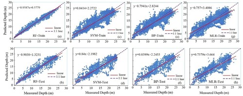
The accuracy of water depth inversion directly affects the final water level and storage change in the lake. With the four water depth inversion methods, the RF, SVM, BP, and MLR methods, the results of bathymetry inversions are described as follows. A comparison was made of the depth that four model inversions based on the Sentinel-2 satellite data made possible and what the in situ measurements provided for QiXiang Co. We used the R², MAE, RMSE, and MRE values to analyse the error and determine the ability to predict and generalize the models. Because the ML model randomly divides the training dataset and test dataset, each training and testing dataset is different. Therefore, we repeated the training and testing for the RF, SVM, and BP models 10 times and took their mean value as the result, which is shown in Table 3 and Figure 3.

Figure 3. Accuracy statistics of the bathymetry models.

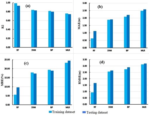
Table 3. Error statistics obtained by comparing the measured value and predicted value from the training and testing datasets.

Model	Training dataset				Testing dataset
	R^2	MAE (m)	RMSE (m)	MRE	R^2	MAE (m)	RMSE (m)	MRE
RF	0.9862	0.63	0.93	5.63%	0.9311	1.13	1.67	9.65%
SVM	0.8372	1.89	2.56	17.89%	0.8247	1.91	2.65	17.3%
BP	0.8134	2.09	2.74	19.4%	0.7977	2.21	2.90	18.9%
MLR	0.759	2.49	3.12	23.3%	0.7418	2.58	3.19	24.5%

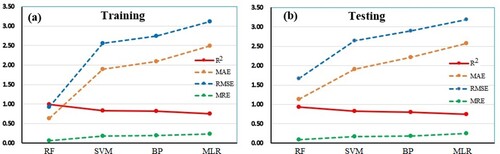
It can be seen that the R² values for RF (R² = 0.9862), SVM (R² = 0.8372), BP (R² = 0.8134), and MLR (R² = 0.7590) that were obtained from the training dataset were always higher than those from the testing dataset. The MAE, RMSE, and MRE values were contrary, which shows that the overall correlation and the accuracy of the fitting data are reasonable. The determination coefficients (R²) of the three machine learning models were higher than those of the MLR model, which indicated a stronger correlation between the water depth simulated values by the machine learning model and the measured water depth values. For the training dataset, the MAE, MRE and RMSE values gradually increased for RF (MAE = 0.63 m, MRE = 5.63% and RMSE = 0.93 m), SVM (MAE = 1.89 m, MRE = 17.89% and RMSE = 2.56 m), and BP (MAE = 2.09 m, MRE = 19.4% and RMSE = 2.74 m), but R² values decreased gradually. In addition, the training dataset showed that the R² values of the four models were slightly higher than those of the testing dataset, but MAE, RMSE, and MRE values were slightly lower than those of the testing dataset. The model’s analysis results for the training and testing dates were consistent. In addition, the R² coefficients for RF were always very close to 1, which was the highest, and MAE, RMSE and MRE values were always the lowest. In Figure 4, there is a very obvious progressive trend in which R² values from the RF, SVM, BP, and MLR models gradually decrease; correspondingly, MAE, RMSE, and MRE values gradually increase.

Figure 4. The trends of R², MAE, RMSE, and MRE values of the training and testing datasets.

Scatterplots of the four model predicted depths from the Sentinel-2 images and the measured depths from the training dataset and testing dataset for QiXiang Co are shown in Figure 5. When the measured data corresponded to the predicted data in the training and testing datasets, collectively, they were located on the y = x line (1:1 line), but the difference appeared in the convergence to the 1:1 line, and the point dispersion was divergent, which indicates that the prediction ability of each model was not the same. For the training dataset, it was obvious that the points of the RF model were the closest to the 1:1 line, and the performance was significantly better than that of the other three models. In addition, for the SVM, BP, and MLR models, we referenced the 1:1 line and the fit line and found that the predicted depth value was higher than the measured depth value in 0–10 m, whereas in 20–28 m, the results were reversed, and in 15–20 m, some points had large errors. For the points that were closer to the 1:1 line, the correlation was higher for the models. In this case, both the training dataset and testing dataset of the RF model were the closest to the 1:1 line, and the plots in the testing set were similar to those in the training set; however, the false degree seemed to be larger in the plots in the testing set than in the training set, which indicates that the RF model was the best model for depth inversion in this study.

Figure 5. Scatterplots of the inversion depth and measured depth from the training and testing datasets with four different models.

The more accurately the depth is inverted, the more accurately the water storage will be estimated for the lake. Therefore, the RF model has acceptable accuracy for analysing the water depth distribution of the lake and can be used further to estimate the change in the water level and storage of the lake.

4.2. Bathymetry maps of the different methods

As shown in Figure 6, we obtained the water depth distribution from different inversion methods. In addition, to compare the effect of the water depth distribution map, spatial interpolation (Topo to Raster) in ArcGIS 10.5 was used to obtain the depth of the lake with grid units of 10 m × 10 m based on bathymetric data. For the spatial interpolation method, we used two methods: one was not to specify the boundary value as level 0 (hereafter referred to as SL), and the other was that the water level at the lakeshore was set as the 0-level by incorporating the outline of the lake as a break line polygon. In the interpolation process, each point along the lakeshore was interpreted as a 0 value (hereafter referred to as SL0). A smoothing filter was applied to the mapping results for visual comparison. Through all of the mapped results, it can be seen that four inversion results basically displayed the overall water depth of the lake; they showed coherent spatial distribution patterns: relatively shallow regions (0–10 m) were located in the near-shore areas, whereas the centre regions had depths more than 10 m. In addition, from the smoothing results of the two kinds of spatial interpolation, we can find obvious divergence: when the boundary value is not set, the interpolation results will be significantly higher where no measured value exists than the actual value; however, when the boundary value is set to 0, the results will be significantly shallower.

Figure 6. Bathymetric maps of QiXiang Co. (a) Derived bathymetry from the RF method. (b) Derived bathymetry from the SVM method. (c) Derived bathymetry from the BP method. (d) Derived bathymetry from the MLR method. (e) Topo to Raster (not set to a 0 value). (f) Topo to Raster (set to a 0 value).

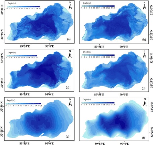
As observed, the depth increased gradually from the northeast and southwest directions to the centre of the lake. The depth of most areas was less than 20 m, and the deepest part was in the centre of the lake. Significant differences occurred in areas with depths of more than 20 m (Figure 6). The four algorithms underestimated the depth values, and for depths deeper than 5 m, the opposite occurred. It is clear that the results of spatial interpolation were the smoothest, followed by the results of the SVM and BP models, while the details of the results from the RF model were the most abundant. Figure 6(a)–(f) and the accuracy analysis of the RF model in Section 3.1 show that RF model-derived bathymetry had an edge over others and produced a good representation of bottom topography and was more accurate.

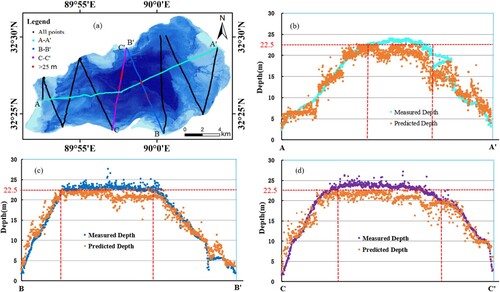
4.3. Analysis of the difference in water depth distribution

To more intuitively reflect the accuracy of the RF model, as shown in Figure 7, the measured depth and the predicted depth of three water depth tracks (A-A’ bright green, B-B’ blue, and C-C’ purple) were compared. From the distribution of measured points, it can be seen that the slope of the A-A’ direction was gentler than that of the B-B’ and C-C’ directions, which is consistent with the shape of the lake. This indicates that the slope gradient was gentle from the A-A’ direction and lower than the B-B’ and C-C’ directions. The difference between the measured depth values and predicted depth values was small and close, and the depth changed slightly from 0 to 22.5 m. The predicted values fluctuated around the measured values, which showed a small error, whereas after a depth of more than 22.5 m, the changes were very gentle, and they had a common phenomenon: the simulated depth was slightly less than the measured depth. In general, the water depth distribution predicted by the RF model was accurate and credible.

Figure 7. Comparison of measured depth and inversion depth from three lines. (a) RF model inversion results and three measured tracks, (b) measured depth vs. predicted depth on A-A’, (c) measured depth vs. predicted depth on B-B’, and (d) measured depth vs. predicted depth on C-C’.

To further compare the accuracy of RF model inversion and spatial interpolation in obtaining water depth where there was no measured value, we removed part of the measured value for the experiment. As shown in Figures 8 and 9, we constructed the RF model and used the spatial interpolation method again to obtain the water depth distribution after removing all measured points in CC’ and B’F. In Figure 6(a) and Figure 8(a), we find that after removing part of the measured values (CC’ and B’F), the bathymetry map of the RF model had almost no change, but compared with Figure 6(e) and Figure 8(b), it was found that the interpolation smoothing results became much higher where there were no measured values from the EF to B’C’ directions, whereas in Figure 6(f) and Figure 9(b), we found that this part of the water depth became shallower. More specifically, the depth values of all measured values and predicted values of CE and EC’ were extracted, as shown in Figure 8(c), Figure 8(d), Figure 9(c), and Figure 9(d), where blue represents the measured depth values (DEPTH), orange represents the inversion depth values of the RF model (RF), and bright green represents the spatial interpolation depth values (SL and SL0). In the CE segment, the depth values obtained by the inversion method and the SL method were in good agreement with the measured values, whereas in EC’ segment, the closer to the lake shore, the larger the error. However, the depth values obtained by the SL method was much lower. These phenomena also intuitively reflects the higher phenomenon than the truth values with no measured points. At the same time, observing the distribution of the three values also reflects the strength and reliability of the RF model inversion in the area without measured values.

Figure 8. The measured values and predicted values of CE and EC’ lines from the RF method and SL method (SL).

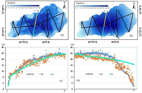
Figure 9. The measured values and predicted values of CE and EC’ lines from the RF method and spatial interpolation method (SL0).

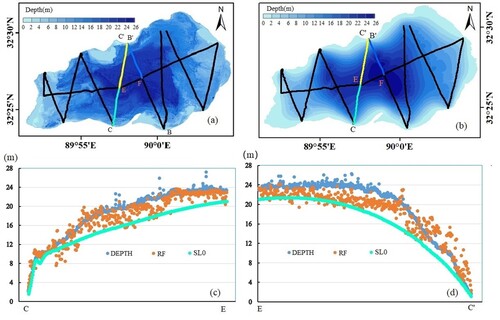
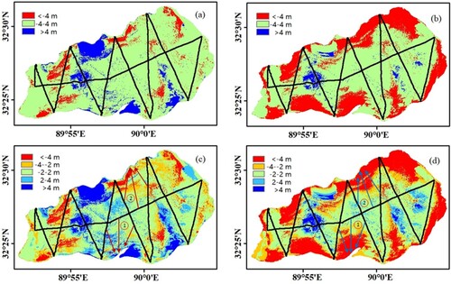
From the above analysis, we know that the overall results of RF model inversion are reliable, while those of the SL method are too large; naturally, those of the SL0 method are too small where and are far from the measured values. To confirm this situation, we took the water depth distribution results from SL and SL0 minus the RF model, and the results are shown in Figure 10. In Figure 10(a) and (b), it can be seen that the difference in most areas was from −4 m to 4 m and was mainly distributed around the measured tracks. Figure 10(b) is more obvious than Figure 10(a), while a larger difference occurred in the edge part where there were no measured values. Moreover, as shown in Figure 10(c) and (d), we further subdivided the difference and found that a range of −2 to 2 m was mainly distributed near the measured points, which could clearly be found in areas 1 and 2. The difference from the measured track to the lake shore direction gradually increased, as shown by the arrow line in Figure 10. In total, we know that the results of the RF model are as reliable as those of spatial interpolation near the measured points, whereas those of the RF model are more accurate than the spatial interpolation results far from the measured values. This indicates that the inversion of water depth by the RF model had a satisfactory accuracy, and it was more accurate than the spatial interpolation method where there were no measured values.

Figure 10. Difference in water depth distribution between spatial interpolation and the RF model. (a) and (c) Distribution of the difference in the water depth between the SL and RF models, (b) and (d) distribution of the difference in the water depth between the SL0 and RF models.

4.4. Dynamic changes in QiXiang Co from 1998 to 2018

4.4.1. Area changes

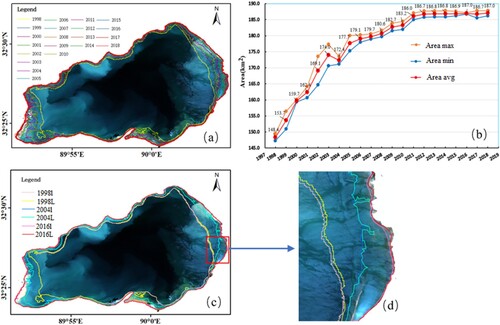
Figure 11(a) shows the minimum boundary of each year from 1998 to 2018, and the horizontal expansion distance of QiXiang Co was calculated based on the minimum boundary. The results showed that the maximum horizontal expansion distance of the lake was 1714.8 m, the average horizontal expansion distance of the lake was 555.3 m, and the average annual horizontal expansion distance of the lake was approximately 27.8 m from 1998 to 2018, which was greater than the pixel resolution of the Sentinel-2 image (10 m × 10 m). Therefore, most boundaries in two consecutive years were located in different pixels. The annual boundary could be converted into discrete points to extract the water depth at the corresponding position as the water level change of the point, and then the mean value of all discrete points could be calculated to represent the average water level change relative to 2018. To be more intuitive, Figure 11(c) demonstrates the maximum boundary and minimum boundary in 2000, 2004, and 2016, and Figure 11(d) is a detailed diagram. It can be clearly seen that the minimum boundary was almost on the inside of the maximum boundary. To improve the representativeness of the average water level change, the maximum boundary and minimum boundary were used to extract the water depth, and then the average value was calculated as the water depth change value. The changes in the maximum area (Area max), minimum area (Area min), and average area (Area avg) are shown in Figure 11(b). The changing trend of the area calculated by the two different boundaries was consistent, and the area calculated by the maximum boundary was always larger than the area calculated by the minimum boundary. From the analysis of the average value of the two, from 1998 to 2018, the area of QiXiang Co continued to expand, from 148.4 km² in 1998 to 187.0 km² in 2018, with a total increase of 38.6 km² and an average annual expansion of 1.93 km². However, there were differences in the growth rate. From 1998 to 2003, the expansion rate was fast, with an average annual expansion of 5.12 km². From 2005 to 2013, the expansion rate decreased slightly, with an annual expansion area of approximately 1.38 km². After 2013, the expansion was slow and entered a stable stage.

Figure 11. Lake shoreline and area change of QiXiang Co. (a) Lake shoreline from 1998 to 2018, (b) area change of QiXiang Co, (c) lake shoreline in three different periods (1999, 2004, and 2016), and (d) partial display.

4.4.2. Water level and storage change analysis from three different methods

According to the analysis in Section 4.4.1, it is feasible to use the lake boundary to extract the water depth as the water level change. Therefore, the maximum boundary and minimum boundary of QiXiang Co from 1998 to 2018 were used to extract the water depth by using the results of RF model inversion and spatial interpolation. In addition, combining the acquired area and the Shuttle Radar Topography Mission (SRTM) DEM (30 m) in 2000, water level and storage changes were estimated separately, and the calculation process was detailed as described in Qiao, Zhu, and Yang (2019). For QiXiang Co, we obtained a linear relationship between the lake surface area and SRTM DEM to estimate the change in elevation value with the change in QiXiang Co’s area from 1998 to 2018, as shown in Equation (13). (13) $y=0.0018\ast x^2-0.4164x+4636.4$(13) where $x$ represents the area, and $y$ represents the corresponding SRTM value.

Figure 12 demonstrates the detailed water level changes of the four methods (RF, SL, SL0, and SRTM) by combining the maximum and minimum boundaries. Table 4 records the average of the water levels obtained from the two boundaries and the water storage changes estimated based on the RF model. The water depth in 2018 was obtained by RF model inversion, and the water level change was regarded as relative to 2018 (the changing value in 2018 was 0), which was obtained by boundary extraction of inversion results. In general, the change in water level obtained by the maximum boundary was always lower, and most pixels had smaller water depths than those obtained by the minimum boundary. The water depth variation values of the four methods (RF, SL, SL0, and SRTM) were 9.36, 8.37, 2.88 and 6.87 m, respectively. From the above analysis, we consider that RF and SL values may have been higher than the actual values, while SL0 values were opposite from 1998 to 2018, but we note that the changes in RF and SRTM values were 7.21 and 6.87 m from 1998 to 2017, respectively, which indicates that the annual average water level changes obtained by the two methods are similar and confirms the reliability of this method. However, for 2017–2018, see Section A of Part V for the causes of high water level changes. In addition, from 1998 to 2003, the variation in water level obtained from RF model inversion was 0.00–3.47 m, with an increased rate of 0.61 m/y. From 2005 to 2013, the variation in the water level was 3.15 m, with an increased rate of 0.39 m/y. After 2013, the water level fluctuated between 2.70 and 2.90 m, indicating that the water level tended to be stable during this period, but the value was relatively high. The reason for this was that RF inversion could lead to a high water depth value in the shallow part. Compared with the variation in water level obtained from spatial interpolation, it was similar to the trend in the area change. Therefore, the water level change obtained by the RF model was used to estimate the water storage change (Figure 13). Water storage had a continuously increasing trend except for 2004, and the water storage increased by 1.811 km³ from 1998 to 2018.

Figure 12. Water level and water storage change from 1998 to 2018 in QiXiang Co. (a) RF, (b) spatial interpolation, (c) SRTM, and (d) average.

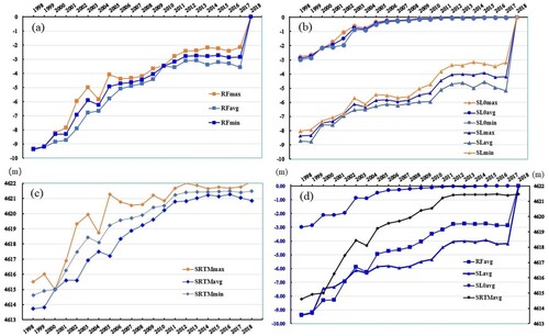
Figure 13. Water storage changes in QiXiang Co.

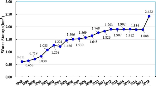
Table 4. Water level and storage change of QiXiang Co in 1998–2018.

Data	RLavg (m)	SLavg (m)	SL0avg (m)	SRTMavg (m)	Volume change (km^3)
1998	−9.36	−8.37	−2.88	4614.61	0.611
1999	−9.18	−8.35	−2.76	4614.92	0.653
2000	−8.31	−7.45	−2.17	4615.00	0.719
2001	−8.29	−7.33	−1.93	4616.25	0.830
2002	−6.95	−6.87	−1.51	4617.46	1.083
2003	−5.89	−6.13	−0.76	4618.43	1.268
2004	−6.26	−6.33	−0.83	4618.11	1.221
2005	−4.94	−5.86	−0.41	4619.23	1.466
2006	−4.74	−5.82	−0.27	4619.56	1.506
2007	−4.63	−5.95	−0.24	4619.71	1.530
2008	−4.46	−5.85	−0.21	4619.91	1.569
2009	−4.05	−5.51	−0.12	4620.41	1.648
2010	−3.47	−5.35	−0.10	4620.53	1.768
2011	−3.18	−4.47	−0.06	4621.23	1.826
2012	−2.77	−4.04	−0.035	4621.41	1.903
2013	−2.75	−4.01	−0.048	4621.43	1.907
2014	−2.78	−4.07	−0.041	4621.43	1.902
2015	−2.72	−3.93	−0.0065	4621.44	1.912
2016	−2.86	−4.21	−0.0065	4621.47	1.884
2017	−2.15	−4.19	−0.0088	4621.40	1.888
2018	0	0	0	4621.48	2.422

5. Discussion

5.1. Accuracy of different depth segments

We analysed the predicted and measured water depth values of the model in deeper and shallower parts and the results then showed that compared with the measured values, the predicted values were larger in shallow areas and smaller in deep areas. To better discuss this phenomenon, the 0–28 m depth of this lake was divided into five different water depth segments. The number of measured points of each segment is shown in Table 5. The water depth (>20 m) was analysed as a segment because of a few points at 25–28 m, and the R², RMSE, MAE, and MRE values for each depth segment were calculated. As shown in Figure 14, the scatterplots of the RF model were mapped with the predicted depth and measured depth, and the results suggested that the RF model had good accuracy in different water depth segments. The R² value was higher than 0.9, and the RMSE value was less than 0.4 m. However, with increasing depth, the RMSE value gradually increased, and the accuracy of the model slightly decreased. Comparing the regression fitting line with the 1:1 line, we clearly found that regardless of the water depth segments, in general, the predicted water depth value of the larger part was slightly less than the measured value, while the predicted value of the smaller part was slightly greater than the measured value, which was similar to the results obtained in Section 3.1. Therefore, if 0–28 m data were used for inversion modelling, the accuracy at 5–20 m was very reliable, which also confirmed that in the shallower part, the inversion value was too high, causing a large change in water level and storage in 2018 compared with 2017 (Figure 12).

Figure 14. Scatter diagrams of the predicted depth vs. the measured depth from different sections.

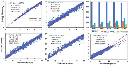
Table 5. The number of different depth segments.

Segment (m)	Mean depth (m)	Number
0–5	3.43	556
5–10	7.80	2947
10–15	12.55	2248
15–20	17.95	1452
20–25	22.49	2552
25–28	25.89	19

5.2. Modelled accuracy analysis

Multispectral remote sensing is mainly based on the transmission of light to water to detect water depth. The value of the visible light attenuation coefficient determines the measurable depth of multispectral remote sensing; the smaller the attenuation coefficient of visible light is, the better the penetration of water. The transmission of visible light in water is mainly limited to 0.4–0.7 μm; when the wavelength range is 0.4–0.6 μm, approximately 50% of the incident radiation can be transmitted, whereas in a wavelength range of 0.6–0.7 μm, it is less than 10%. Once the turbidity of the waterbody increases, the backscattering component of water will soon be greater than the reflection component from the bottom. When the turbidity of the waterbody is more uniform, the backscattering component of water has a good positive correlation with the depth of the waterbody, which can also estimate water depth. Regardless of pure water, ocean water, or coastal water, the minimum value of the visible light attenuation coefficient appears in the blue–green band, and the penetration of the blue and green bands in the water is the best (Xia et al. 2020). Table 2 shows that the correlation coefficients of water depth and band reflectance are higher in the coastal aerosol (b1), blue (b2), green (b3), and red (b4) bands, and the wavelengths range from 0.4 to 0.7 μm. When the water becomes turbid, the minimum value of the attenuation coefficient will move to the side of wavelength, and the highest correlation coefficient is in the green (b3) band, which is consistent with the complex composition of lake water and unclear water.

Furthermore, in this research, the logarithm and logarithm ratio of band reflectivity were used as modelling factors, which takes into account the complexity of lake sediment changes and the great change in clarity. The multiband linear combination was proposed by Lyzenga using two or more different bands, which can drastically avoid the lack of optical characteristics of the water, assumes a constant reflectivity at the bottom of the waterbody, and ignores the distinctiveness of the sediments (Lyzenga 1985). The two-band ratio was established by Stumpf for shallow water depth information. The formulas of the Lyzenga model and Stumpf model are shown in Equations (1) and (2). To prove that this special combination can effectively improve the inversion accuracy, three models were compared, and the results are shown in Table 6. This confirmed the rationality of the factor combination.

Table 6. Error statistics of the MLR, Stumpf and Lyzenga models.

	R^2	MAE	RMSE	MRE
Stumpf	0.707	2.73	3.44	25.60%
Lyzenga	0.7243	2.66	3.33	24.80%
MLR	0.7574	2.49	3.12	23.30%

In addition, the optimization of model parameters is helpful in improving the accuracy of water depth inversion. The three machine learning models were realized by utilizing the library in Python 3.8, and there were deficiencies in the setting and optimization of the parameters. For instance, the number of middle layers in the BP model, the number of neurons and the kernel function in the SVM model, the number of decision trees in the RF model, the maximum tree depth, the maximum penalty coefficient, etc., have a vital role in the accuracy of each model. Limited by the measured data, this experiment only carried out an inversion experiment on one lake and did not carry out inversion research on the water depth of other lakes with the same water quality and sediment. Therefore, the fitting model will be used to carry out an inversion test in other study areas to verify the universality of the inversion method in the estimation of lake water level and water volume on the Tibetan Plateau.

6. Conclusion

In the study of water resources on the TP, it is very important to obtain high-precision water depth and water level data of lakes, and in water depth inversion, the prediction performance of different inversion models is different in specific areas. In this study, we used the logarithm of band reflectance and its ratio as model input to evaluate the performance of three machine learning models (RF, SVM, and BP) and MLR models in lake water depth prediction and acquired the change in water level and storage based on satellite imagery and bathymetric data of QiXiang Co. The model clearly showed different estimates of water depth, the accuracy of the three machine learning models was higher than that of the MLR model, and the RF model had the most powerful water depth simulation ability among these models. In the bathymetric maps, different models demonstrated a consistent trend of water depth distribution, the water depth distribution results were more abundant and detailed using the RF model, and the inversion of the overall water depth of the lake using the RF model had the best accuracy and performance. In particular, where there was no measured value distribution, and the prediction results of the RF model were more accurate than those of spatial interpolation. Moreover, the water level increased by approximately 9.36 m (0.47 m/y) based on the RF model inversion depth.

In summary, ML models have good performance in lake water depth inversion, and remote sensing water depth inversion has an acceptable accuracy compared with the water level and storage estimates made by the spatial interpolation and DEM methods. In future work, the water depth estimation accuracy can be improved through adjusted model inputs and parameter models and segmented inversion of water depth, and more lake bathymetric data are needed to verify the universality of the models and the accuracy of estimating the water level and water storage of shallow lakes based on the inversion water depth.

Acknowledgments

This work is supported by the Second Tibetan Plateau Scientific Expedition and Research (STEP) (2019QZKK0202), NSFC project (41831177, 41901078), 2020 Science and technology project of innovation ecosystem construction, National Supercomputing Zhengzhou center-Research on Key Technologies of intelligent fine prediction based on big data analysis (201400210800), CAS Strategic Priority Research Program (XDA19020303, XDA20020100), the Ministry of Science and Technology of China Project (2018YFB05050000), and the CAS Alliance of Field Observation Stations (KFJ-SW-YW038).

Data availability statement

The data that support the findings of this study are openly available in ‘figshare’ at http://doi.org/10.6084/m9.figshare.17348660.

Disclosure statement

No potential conflict of interest was reported by the author(s).

Additional information

Funding

This work was supported by 2020 Science and technology project of innovation ecosystem construction, National Supercomputing Zhengzhou center-Research on Key Technologies of intelligent fine prediction based on big data analysis [grant number: 201400210800]; Second Tibetan Plateau Scientific Expedition and Research (STEP) [grant number: 2019QZKK0202]; the CAS Alliance of Field Observation Stations [grant number: KFJ-SW-YW038]; CAS Strategic Priority Research Program: [Grant Number XDA19020303, XDA20020100]; the Ministry of Science and Technology of China Project [grant number: 2018YFB05050000]; National Natural Science Foundation of China project [grant number: 41831177, 41901078].

References

- Becker, J. J., D. T. Sandwell, W. H. F. Smith, J. Braud, B. Binder, J. Depner, D. Fabre, et al. 2009. “Global Bathymetry and Elevation at 30 Arc Seconds Resolution: SRTM30_PLUS.” Marine Geodesy 32 (4): 355–371. doi:10.1080/01490410903297766.
- Brando, V. E., J. M. Anstee, M. Wettle, A. G. Dekker, S. R. Phinn, and C. Roelfsema. 2009. “A Physics Based Retrieval and Quality Assessment of Bathymetry from Suboptimal Hyper Spectral Data.” Remote Sensing of Environment 113 (4): 755–770. doi:10.1016/j.rse.2008.12.003.
- Breiman, L. 2001. “Random Forests.” Machine Learning 45: 5–32. doi:10.1023/A:1010933404324.
- Caballero, I., and R. P. Stumpf. 2019. “Retrieval of Nearshore Bathymetry from Sentinel-2A and 2B Satellites in South Florida Coastal Waters.” Estuarine, Coastal and Shelf Science 226: 106277. doi:10.1016/j.ecss.2019.106277.
- Chénier, R., M. A. Faucher, and R. Ahola. 2018. “Satellite-Derived Bathymetry for Improving Canadian Hydrographic Service Charts.” ISPRS International Journal of Geo-Information 7 (8): 306–321. doi:10.3390/ijgi7080306.
- Clarke, S. M., J. H. Griebsch, and T. W. Simpson. 2005. “Analysis of Support Vector Regression for Approximation of Complex Engineering Analyses.” Journal of Mechanical Design 127: 1077–1087. doi:10.1115/1.1897403.
- Costa, B. M., T. A. Battista, and S. J. Pittman. 2009. “Comparative Evaluation of Airborne LiDAR and Ship-Based Multibeam SoNAR Bathymetry and Intensity for Mapping Coral Reef Ecosystems.” Remote Sensing of Environment 113: 1082–1100. doi:10.1016/j.rse.2009.01.015.
- Dierssen, H. M., R. C. Zimmerman, R. A. Leathers, T. V. Downes, and C. O. Davis. 2013. “Ocean Color Remote Sensing of Seagrass and Bathymetry in the Bahamas Banks by High-Resolution Airborne Imagery.” Limnology and Oceanography 48 (1): 444–455. doi:10.4319/lo.20033.48.1_part_2.0444.
- Ebtehaj, I., and H. Bonakdari. 2016. “A Support Vector Regression-Firefly Algorithm-Based Model for Limiting Velocity Prediction in Sewer Pipes.” Water Science and Technology 73 (9): 2244–2250. doi:10.2166/wst.2016.064.
- Eugenio, F., J. Marcello, and J. Martin. 2015. “High-Resolution Maps of Bathymetry and Benthic Habitats in Shallow-Water Environments Using Multispectral Remote Sensing Imagery.” IEEE Transactions on Geoscience and Remote Sensing 53: 3539–3549. doi:10.1109/TGRS.2014.2377300.
- European Space Agency. 2021a. “ESA Sentinel 2 Orbit Description.” Accessed September 2, 2021. https://sentinel.esa.int/web/sentinel/missions/sentinel-2/satellite-description/orbit.
- European Space Agency. 2021b. “Sentinel-2 MSI Technical Guide.” Accessed September 2, 2021. https://earth.esa. int/web/sentinel/technical-guides/sentinel-2-msi.
- Geladi, P., and B. R. Kowalski. 1986. “Partial Least-Squares Regression: A Tutorial.” Analytica Chimica Acta 185: 1–17. doi:10.1016/0003-2670(86)80028-9.
- Getirana, A., H. C. Jung, and K. Tseng. 2018. “Deriving Three Dimensionals Reservoir Bathymetry from Satellite Datasets.” Remote Sensing of Environment 217: 366–374. doi:10.1016/j.rse.2018.08.030.
- Han, Z., X. Zhu, X. Fang, Z. Wang, L. Wang, G. Zhao, and Y. Jiang. 2016. “Hyperspectral Estimation of Spple Tree Canopy LAI Based on SVM and RF Regression.” Spectrosc Spectr Anal 36 (3): 800–805. doi:10.3964/j.issn.1000-0593(2016)03-0800-06.
- Hedley, J. D., C. Roelfsema, I. Chollett, A. Harborne, S. Heron, S. Weeks, et al. 2016. “Remote Sensing of Coral Reefs for Monitoring and Management: A Review.” Remote Sensing 8 (2): 118. doi:10.3390/rs8020118.
- Hodúl, M., S. Bird, A. Knudby, and R. Chénier. 2018. “Satellite Derived Photogrammetric Bathymetry.” ISPRS Journal of Photogrammetry and Remote Sensing 142: 268–277. doi:10.1016/j.isprsjprs.2018.06.015.
- Iverson, L. R., A. M. Prasad, S. N. Matthews, and M. Peters. 2008. “Estimating Potential Habitat for 134 Eastern US Tree Species Under Six Climate Scenarios.” Forest Ecology and Management 254 (3): 390–406. doi:10.1016/j.foreco.2007.07.023.
- Jiang, L., K. Nielsen, O. B. Andersen, and P. Bauer-Gottwein. 2020. “A Bigger Picture of How the Tibetan Lakes Have Changed Over the Past Decade Revealed by CryoSat-2 Altimetry.” Journal of Geophysical Research: Atmospheres 125 (23). doi:10.1029/2020JD033161.
- Khoshnevisan, B., S. Rafiee, and M. Omid. 2013. “Prognostication of Environmental Indices in Potato Production Using Artificial Neural Networks.” Journal of Cleaner Production 52: 402–409. doi:10.1016/j.jclepro.2013.03.028.
- Kranjcic, N., D. Medak, R. Zupan, and M. Rezo. 2019. “Support Vector Machine Accuracy Assessment for Extracting Green Urban Areas in Towns.” Remote Sensing 11 (6): 655. doi:10.3390/rs11060655.
- Kutser, T., J. Hedley, C. Giardino, C. Roelfsema, and V. E. Brando. 2020. “Remote Sensing of Shallow Waters – A 50 Year Retrospective and Future Directions.” Remote Sensing of Environment 240: 111619. doi:10.1016/j.rse.2019.111619.
- Lacaux, J. P., Y. M. Tourre, C. Vignolles, J. A. Ndione, and M. Lafaye. 2007. “Classification of Ponds from High-Spatial Resolution Remote Sensing: Application to Rift Valley Fever Epidemics in Senegal.” Remote Sensing of Environment 106 (1): 66–74. doi:10.1016/j.rse.2006.07.012.
- Li, J. W., D. Knapp, M. Lyons, C. Roelfsema, S. Phinn, S. Schill, et al. 2021. “Automated Global Shallow Water Bathymetry Mapping Using Google Earth Engine.” Remote Sensing 13 (8): 1469. doi:10.3390/rs13081469.
- Li, Y., J. Liao, H. Guo, Z. Liu, and G. Shen. 2014. “Patterns and Potential Drivers of Dramatic Changes in Tibetan Lakes, 1972–2010.” PloS One 9 (11): e111890. doi:10.1371/journal.pone.0111890.
- Liu, Z. 2013. “Bathymetry and Bottom Albedo Retrieval Using Hyperion: A Case Study of Thitu Island and Reef.” Chinese Journal of Oceanology and Limnology 31: 1350–1355. doi:10.1007/s00343-013-2287-8.
- Liu, S., L. Wang, H. Liu, H. Su, X. Li, and W. Zheng. 2018. “Deriving Bathymetry from Optical Images With a Localized Neural Network Algorithm.” IEEE Transactions on Geoscience and Remote Sensing 56 (9): 5334–5342. doi:10.1109/TGRS.2018.2814012.
- Lyzenga, D. R. 1978. "Passive Remote Sensing Techniques for Mapping Water Depth and Bottom Features." Applied Optics 17 (3): 379–383. doi: 10.1364/AO.17.000379.
- Lyzenga, D. R. 1985. “Shallow-Water Bathymetry Using Combined Lidar and Passive Multispectral Scanner Data.” International Journal of Remote Sensing 6: 115–125. doi:10.1080/01431168508948428.
- Ma, H., and S. Liu. 2016. “The Potential Evaluation of Multisource Remote Sensing Data for Extracting Soil Moisture Based on the Method of BP Neural Network.” Canadian Journal of Remote Sensing 42 (2): 117–124. doi:10.1080/07038992.2016.1160773.
- Mas, J. F., and J. J. Flores. 2008. “The Application of Artificial Neural Networks to the Analysis of Remotely Sensed Data.” International Journal of Remote Sensing 29 (3): 617–663. doi:10.1080/01431160701352154.
- Mateo-Pérez, V., M. Corral-Bobadilla, F. Ortega-Fernández, and E. P. Vergara-González. 2020. “Port Bathymetry Mapping Using Support Vector Machine Technique and Sentinel-2 Satellite Imagery.” Remote Sensing 12 (13): 2069. doi:10.3390/rs12132069.
- Misra A., Z. Vojinovic, B. Ramakrishnan, A. Luijendijk, and R. Ranasinghe. 2018. "Shallow Water Bathymetry Mapping using Support Vector Machine (SVM) Technique and Multispectral Imagery.” International Journal of Remote Sensing 39 (13): 4431-4450. doi: 10.1080/01431161.2017.1421796.
- Mukherjee, L., P. Zhai, M. Gao, Y. X. Hu, B. A. Franz, and J. P. Werdell. 2020. “Neural Network Reflectance Prediction Model for Both Open Ocean and Coastal Waters.” Remote Sensing 12 (9): 1421. doi:10.3390/rs12091421.
- Mutanga, O., E. Adam, and M. A. Cho. 2012. “High Density Biomass Estimation for Wetland Vegetation Using WorldView-2 Imagery and Random Forest Regression Algorithm.” International Journal of Applied Earth Observation and Geoinformation 18 (1): 399–406. doi:10.1016/j.jag.2012.03.012.
- Mynett, A. E., and Z. Vojinovic. 2009. “Hydroinformatics in Multi-Colours—Part Red: Urban Flood and Disaster Management.” Journal of Hydroinformatics 11 (3–4): 166–180. doi:10.2166/hydro.2009.027.
- Phan, V. H., R. Lindenbergh, and M. Menenti. 2012. “ICESat Derived Elevation Changes of Tibetan Lakes Between 2003 and 2009.” International Journal of Applied Earth Observation and Geoinformation 17: 12–22. doi:10.1016/j.jag.2011.09.015.
- Qiao, B. J., L. P. Zhu, J. B. Wan, J. J. Ju, Q. F. Ma, L. Huang, et al. 2019. “Estimation of Lake Water Storage and Changes Based on Bathymetric Data and Altimetry Data and the Association With Climate Change in the Central Tibetan Plateau.” Journal of Hydrology 578: 124052. doi:10.1016/j.jhydrol.-2019.124052.
- Qiao, B. J., L. P. Zhu, J. B. Wan, J. T. Ju, Q. F. Ma, and C. Liu. 2017. “Estimation of Lakes Water Storage and Their Changes on the Northwestern Tibetan Plateau Based on Bathymetric and Landsat Data and Driving Force Analyses.” Quaternary International 454: 56–67. doi:10.1016/j.quaint.2017.08.005.
- Qiao, B., L. Zhu, and R. Yang. 2019. “Temporal-Spatial Differences in Lake Water Storage Changes and Their Links to Climate Change Throughout the Tibetan Plateau.” Remote Sensing of Environment 222: 232–243. doi:10.1016/j.rse.2018.12.037.
- Roy, D. P., M. A. Wulder, T. R. Loveland, C. E. Woodcock, R. G. Allen, M. C. Anderson, et al. 2014. “Landsat-8: Science and Product Vision for Terrestrial Global Change Research.” Remote Sensing of Environment 145: 154–172. doi:10.1016/j.rse.2014.02.001.
- Sandidge, J. C., and R. J. Holyer. 1998. “Coastal Bathymetry from Hyperspectral Observations of Water Radiance.” Remote Sensing of Environment 65 (3): 341–352. doi:10.1016/S00344257(98)00043-1.
- Song, C., B. Huang, and L. Ke. 2013. “Modeling and Analysis of Lake Water Storage Changes on the Tibetan Plateau Using Multi-Mission Satellite Data.” Remote Sensing of Environment 135: 25–35. doi:10.1016/j.rse.2013.03.013.
- Song, C., B. Huang, L. Ke, and K. S. Richards. 2014. “Seasonal and Abrupt Changes in the Water Level of Closed Lakes on the Tibetan Plateau and Implications for Climate Impacts.” Journal of Hydrology 514: 131–144. doi:10.1016/j.jhydrol.2014.04.018.
- Stumpf, R. P., K. Holderied, and M. Sinclair. 2003. “Determination of Water Depth with High-Resolution Satellite Imagery Over Variable Bottom Types.” Limnology and Oceanography 48 (1): 547–556. doi:10.4319/lo.2003.48.1_part_2.0547.
- Su, H., H. Liu, and W. D. Heyman. 2008. “Automated Derivation of Bathymetric Information from Multi-Spectral Satellite Imagery Using a Non-Linear Inversion Model.” Marine Geodesy 31 (4): 281–298. doi:10.1080/01490410802466652.
- Sun, L., and K. Schulz. 2015. “The Improvement of Land Cover Classification by Thermal Remote Sensing.” Remote Sensing 7: 8368–8390. doi:10.3390/rs70708368.
- Wan, J., and Y. Ma. 2021. “Shallow Water Bathymetry Mapping of Xinji Island Based on Multispectral Satellite Image Using Deep Learning.” Journal of the Indian Society of Remote Sensing 49 (9): 2019–2032. doi:10.1007/s12524-020-01255-9.
- Wang L., H. X. Liu, H. X. B. Su, and J. Wang. 2019. “Bathymetry Retrieval from Optical images with Spatially Distributed Support Vector Machines.” GIScience and Remote Sensing 56 (3): 323-337. doi: 10.1080/15481603.2018.1538620.
- Wechsler, S. 2007. “Uncertainties Associated With Digital Elevation Models for Hydrologic Applications: A Review.” Hydrology and Earth System Sciences 11 (4): 1481–1500. doi:10.5194/hess-11-1481-2007.
- Wolter, P. T., P. A. Townsend, B. R. Sturtevant, and C. C. Kingdon. 2008. “Remote Sensing of the Distribution and Abundance of Host Species for Spruce Budworm in Northern Minnesota and Ontario.” Remote Sensing of Environment 112 (10): 3971–3982. doi:10.1016/j.rse.2008.07.005.
- Xia, H. Y., X. R. Li, H. G. Zhang, J. Wang, X. L. Lou, K. G. Fan, et al. 2020. "A Bathymetry Mapping Approach Combining logratio and Semianalytical Models using four-band Multispectral Imagery without Ground Data." IEEE Transactions on Geoscience and Remote Sensing 58 (4): 2695-2709. doi:10.1109/TGRS.2019.2953381.
- Yang, N., J. H. Li, W. B. Mo, W. J. Luo, D. Wu, W. C. Gao, and C. M. Sun. 2020. “Water Depth Retrieval Models of East Dongting Lake, China, Using GF-1 Multi-Spectral Remote Sensing Images.” Global Ecology and Conservation 22: e1004. doi:10.1016/j.gecco.2020.e01004.
- Yang, K., H. Wu, J. Qin, C. Lin, W. Tang, and Y. Chen. 2014. “Recent Climate Changes Over the Tibetan Plateau and Their Impacts on Energy and Water Cycle: A Review.” Global and Planetary Change 112: 79–91. doi:10.1016/j.gloplacha.2013.12.001.
- Yunus, A. P., J. Dou, X. Song, and R. Avtar. 2019. “Improved Bathymetric Mapping of Coastal and Lake Environments Using Sentinel-2 and Landsat-8 Images.” Sensors 19 (12): 2788. doi:10.3390/s19122788.
- Zhang, G., H. Xie, T. Yao, and S. Kang. 2013. “Water Balance Estimates of Ten Greatest Lakes in China Using ICESat and Landsat Data.” Chinese Science Bulletin 58 (31): 3815–3829. doi:10.1007/s11434-013-5818-y.
- Zhou T., F. Wang, and Z. Yang. 2017. “Comparative Analysis of ANN and SVM Models Combined with Wavelet Preprocess for Groundwater Depth Prediction.” Water 9 (10): 781. doi: 10.3390/w9100781.