A real 3D scene rendering optimization method based on region of interest and viewing frustum prediction in virtual reality

ABSTRACT

As an important technology of digital construction, real 3D models can improve the immersion and realism of virtual reality (VR) scenes. The large amount of data for real 3D scenes requires more effective rendering methods, but the current rendering optimization methods have some defects and cannot render real 3D scenes in virtual reality. In this study, the location of the viewing frustum is predicted by a Kalman filter, and eye-tracking equipment is used to recognize the region of interest (ROI) in the scene. Finally, the real 3D model of interest in the predicted frustum is rendered first. The experimental results show that the method of this study can predict the frustrum location approximately 200 ms in advance, the prediction accuracy is approximately 87%, the scene rendering efficiency is improved by 8.3%, and the motion sickness is reduced by approximately 54.5%. These studies help promote the use of real 3D models in virtual reality and ROI recognition methods. In future work, we will further improve the prediction accuracy of viewing frustums in virtual reality and the application of eye tracking in virtual geographic scenes.

KEYWORDS:

• Real 3D scene
• virtual reality
• Kalman filter
• region of interest
• viewing frustum

1 Introduction

Real 3D models are widely used in urban planning, 3D navigation, training, scientific research and other fields (Verhoeven 2011; Lin, Li, and Zhou 2020; Zhang et al. 2020). Real 3D models have the characteristics of better realism, rich details and convenient data acquisition (Li et al. 2018a; Wang et al. 2020), and they are the key technical support of three-dimensional expressions in the construction of digital earth. An increasing number of 3D scenes have begun to use real 3D models instead of other modeling methods, especially in virtual reality (VR) scenes. VR technology is one of the tools to study virtual geographic environments (Lin, Chen, and Lu 2013; Chen et al. 2013), and with the characteristics of immersion, interaction and imagination, it can provide users with visual, auditory and perceptual virtual experiences. Compared with traditional manual modeling scenes, real 3D scenes can provide a more realistic environment for VR and greatly improve visual immersion (Lin et al. 2015; Tibaldi et al. 2020; Cai et al. 2021), which is the foundation and core of VR technology (Checa and Bustillo 2020).

As unmanned aerial vehicle (UAV) oblique photography technology has progressed, the acquisition of real 3D model data has become more efficient and convenient (Lingua et al. 2017), and the model resolution and texture resolution have been greatly improved (Zhou et al. 2021; Xu et al. 2021). More sophisticated models also bring a larger amount of data (Yijing and Yuning 2018), and the amount of real 3D data is thousands of times that of manual modeling data, which puts forward higher requirements for binocular parallel rendering in VR (Patney et al. 2016; Konrad, Angelopoulos, and Wetzstein 2020).

At present, to optimize real 3D scene rendering in virtual reality, more attention is given to how to make computers draw finer or wider scenes with limited hardware resources, and the visual characteristics of human eyes and the characteristics of the virtual reality observation mode are not considered. In practice, when users observe a virtual scene, their eyes will preferentially search for and locate a more general region of interest (ROI) (Purucker et al. 2013; Ho 2014; Sun et al. 2020). Especially in virtual reality, the movement of a helmet-mounted display (HMD) determines the user's observation region and the ROI range of their eyes. Although some studies have also tried to use eye tracking to optimize the rendering of virtual geographic scenes, these methods are not suitable for real 3D scenes. Therefore, how to optimize real 3D scene rendering by using special interaction methods such as virtual reality and human visual characteristics has become an important research topic.

To solve the above problems, this study proposes an ROI recognition method based on eye tracking in VR and uses a Kalman filter to predict a user’s viewing frustum. Finally, we constructed a VR prototype system and conducted experiments to verify the method.

2 Background

Virtual reality is a kind of Extended Reality (X-Reality, XR) technology. XR technology refers to the human–computer interaction environment that integrates the real and virtual environments through computer hardware and wearable technology (Alizadehsalehi, Hadavi, and Huang 2020). XR includes VR, AR (Augmented reality) and MR (Mixed reality). XR technology is the basic support and carrier of metaverses, which can provide more convenience and possibilities in work, education, entertainment and so on. In particular, VR technology has become the most mature and widely used technology in XR due to its lower system and technical complexity (Li et al. 2018b). However, the binocular rendering method of virtual reality requires that scenes be rendered from two angles at the same time (Huang, Chen, and Zhou 2020). This rendering pressure is approximately twice that of a traditional computer screen. Furthermore, VR's stronger sense of immersion causes motion sickness, especially for virtual scenes that need to render a large amount of geographic data (Billen et al. 2008). Motion sickness has become an important factor that hinders users from exploring and interacting with virtual geographic scenes (Kim et al. 2018). Enhancing the rendering efficiency of virtual scenes is an effective means to reduce the occurrence of motion sickness and improve the user experience (Chang, Kim, and Yoo 2020).

Generally, there are two ways to improve the rendering efficiency of virtual scenes:

1. The 3D model in the scene can be optimized to reduce the number of vertices rendered by the computer (Asgharian and Ebrahimnezhad 2020). Delaunay triangulation is the most commonly used terrain data model (Sibson 1978). Early studies focused on expressing more accurate terrain with fewer triangles, including the divide and conquer approach (Dwyer 1987), iterative method (Lee and Schachter 1980), sweep line algorithm (Fortune 1987), minimum-weight triangulation method (Lingas 1986), and bagging-based algorithm (Su and Drysdale 1997). These methods are very mature and widely used. However, with the development of 3D visualization technology, 3D data models have become the main expression of terrain and geographic features. Researchers have begun studying the optimization method of 3D geographic data models. Examples include the hierarchical shape analysis and iterative edge algorithm (Van, Shi, and Zhang 2004), the white optimization algorithm (Liang, He, and Zeng 2020), the evolutionary multi-objective algorithm (Campomanes-Álvarez, Cordon, and Damas 2013), and parallel computing to quickly simplify the model (Cabiddu and Attene 2015; Konrad, Angelopoulos, and Wetzstein 2020). These algorithms simplify the 3D model by preserving visual features and finally improve the efficiency of geographic scene rendering. However, simplifying the 3D model inevitably leads to a decline in the visual effect, which is a trade-off between the visual effect and rendering performance.

2. The rendering strategy of the 3D geographic scene can be optimized to maximize the rendering efficiency of the computer. For example, the rendering strategy is changed according to the characteristics of computer hardware. Zhang used the hybrid rendering method of servers and clients to improve the rendering efficiency of large-scale building scenes (Zhang et al. 2014). Hu used small tile data to improve the rendering effect of flood scenes according to the characteristics of mobile virtual reality (Hu et al. 2018). Dang and Zhang use graphics processing units (GPUs) to render large-scale terrain and disaster scenes (Zhang et al. 2019; Zhang et al. 2021; Dang et al. 2021). This kind of method improves the scene rendering effect by further improving the use efficiency of computer hardware, but the performance of computer hardware is limited, which leads to the limited improvement of the final scene rendering effect. In addition, according to the virtual scene rendering strategy of human eye characteristics, Duchowski used a foveated continuous gaze approach to optimize the scene rendering effect (Duchowski and Çöltekin 2007), and Fu reduced the rendering effect of non-concerned flood regions through tunnel vision (Fu et al. 2021). This kind of method began to consider the visual characteristics of human eyes and achieved a certain optimization effect. However, their optimization area is static, and the human eye attention area is not read in real time, which leads to the difference between the actual human eye attention area and their optimization area. Although the efficiency of scene rendering has been improved, the actual visual quality of users has not been improved.

Using eye tracking to render virtual scenes in real time is a more reasonable method. The response of eye-tracking equipment has a delay of 15–52 ms (Stein et al. 2021), and Albert believes that the rendering delay of eye movement and attention should be kept within 50–70 ms, which is acceptable to users (Albert et al. 2017). In ordinary virtual scenes, the rendering delay of the ROI is acceptable (Lee et al. 2020; Meng, Du, and Varshney 2020), and good optimization results are achieved. However, in a real 3D virtual scene, due to the large amount of fine data, rendering the real 3D models directly according to an eye-tracking device will make users uncomfortable and reduce the user experience. Therefore, how to apply the eye-tracking method to render real 3D scenes in virtual reality has become a problem to be studied.

3 Methodology

3.1 Research framework overview

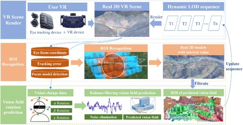
First, we obtain a user's observation region of a scene through a VR eye-tracking device and calculate the user’s interest value in each region. These values of interest are classified using cluster analysis and cumulative recorded in the corresponding real 3D models. During observation, a Kalman filter is used to predict the rotation of the user’s VR helmet, and the viewing frustum of the user at the next time is obtained. Finally, the real 3D model in the predictive viewing frustum is loaded into memory in advance and rendered in turn according to the interest value (Figure 1).

Figure 1. Overview of the research framework.

3.2 ROI recognition in real 3D scenes based on eye tracking

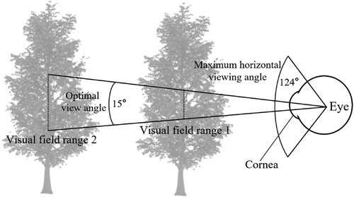
Humans have a variety of perceptual modalities, among which visual perception accounts for approximately 70% of overall perception, so vision is decisive for immersion in VR (Stein et al. 1996; Vignais et al. 2015). The horizontal visual field extent of both eyes in humans is approximately 220°, the vertical visual field is approximately 135°, and the coincident visual field is approximately 124° in both eyes (Atchison and Thibos 2016). Information can be correctly identified within approximately 15° of the effective viewing region of the human eye, so the effective viewing region of the human eye can be regarded as the ROI (Clay, König, and Koenig 2019). As the viewing distance grows, the ROI gradually becomes larger, as shown in Figure 2.

Figure 2. Human visual characteristics.

When viewing a real 3D scene in VR, different viewing distances and viewing times will lead to different cognitive effects, meaning different levels of interest. With increasing viewing distance, the viewing range will increase, while the cognitive effects of the objects in the range will decrease. With increasing viewing time, the cognitive effects will improve, although the improvement is limited. This means that at a distance, where the observer's eye is looking is not necessarily an ROI. When the eyes locate an ROI, they will observe these regions discretely, which is called saccade (Deubel and Schneider 1996; Findlay 1997), Saccade is often irregular and difficult to predict because the average time of saccade is 20–40 ms and the speed can reach 600°/s (Baloh et al. 1975; Wooding 2002). Therefore, this study predicts the viewing frustum instead of the ROI and then uses the ROI of the previous observer as the priority rendering region of the observer this time.

To measure whether a region in a real 3D scene is an ROI, a VR eye-tracking device can be used to measure whether the human eye is interested in a region through Formula 1. (1) $\mathrm{\partial }={\displaystyle \frac{D_t(\mathrm{Ma}{\mathrm{x}}_d-\mathrm{Mi}{\mathrm{n}}_d)}{D_d(\mathrm{Ma}{\mathrm{x}}_t-\mathrm{Mi}{\mathrm{n}}_t)}}$(1) where $\mathrm{\partial }$ represents the degree of interest, $D_t$ represents the time to observe a region, and $D_d$ represents the distance when the region is observed. $\mathrm{Ma}{\mathrm{x}}_d$ and $\mathrm{Mi}{\mathrm{n}}_d$ indicate the maximum and minimum distances between the observer and the real 3D model, respectively, during the entire observation period. $\mathrm{Ma}{\mathrm{x}}_t$ and $\mathrm{Mi}{\mathrm{n}}_t$ indicate the longest and shortest times, respectively, for the observer to observe a certain region during the observation period. Formula 1 can only reflect the ratio of time to distance. However, under the condition of a certain model resolution, observation distances that are too close or too far will cause deviations when using Formula 1, which will affect the division of the ROI. In this situation, this study combines the human visual characteristics and the imaging principle of VR equipment and corrects it using Formula 2. (2) $\begin{array}{c}\{\begin{array}{c}{D}_d>{\displaystyle \frac{w\alpha R}{2Fov\cdot \tan \left({\displaystyle \frac{\alpha }{2}}\right)},\mathrm{\partial }=0}\\ D_d<{\displaystyle \frac{R}{2\tan \left({\displaystyle \frac{\alpha }{2}}\right)},\mathrm{\partial }=0}\end{array}\end{array}$(2) where $w$ is the resolution of the VR device, $\alpha$ is the effective observation angle of the human eye, generally taken as 15°, $R$ is the spatial resolution of the real 3D model of the observation region, and $Fov$ is the maximum field of view of the VR device. When the distance is too far and the region of each pixel in the observer's best view is smaller than the real 3D model resolution, the observation is considered invalid. When the distance is too close, the region of all pixel points in the observer’s view is equal to the terrain resolution, so the observation is considered invalid and the $\mathrm{\partial }$ value is guaranteed to be within a certain and reasonable range using Formula 2.

Real 3D model data are often irregular. To better detect the eye movement observation region and divide the ROI, this study uses a 3D grid with an edge length of L to divide the real 3D scene. Each 3D grid has ϵ, and the initial value is 0. The value of L is determined by the spatial resolution and empirical value of the real 3D model. The value of L can be larger when the model is rough and smaller when the resolution is higher. A smaller L means that the scene is divided more finely, requires more memory, and is less efficient to retrieve. Therefore, the minimum value of L should be greater than or equal to the minimum outer enclosure side length of the real 3D model in the scene. Too small an L value is meaningless for scene partitioning and will only increase the performance overhead (Figure 3).

Figure 3. ROI recognition of a real 3D scene.

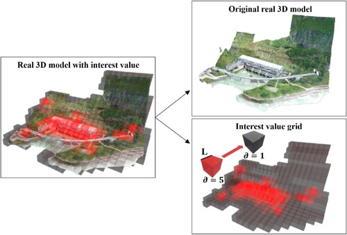
When the focus range of the observer's eyes intersects with the 3D grid, the time and observation distance when the focus region overlaps with the 3D grid are recorded. After the observation, the $\mathrm{\partial }$ value is calculated according to Formulas 1 and 2 and $\mathrm{\partial }$ accumulates to the corresponding ϵ.

The model rendering order of the current scene is calculated using the cumulative value of interest of all previous users. Different users may have the same interest in a region, but different users have different $\mathrm{\partial }$ values in the region. If the $\mathrm{\partial }$ value is directly accumulated to ϵ, ϵ cannot correctly reflect the degree of interest. Therefore, it is necessary to standardize the value of interest of each user in each region. To standardize the interest values of different users, this study uses the Jenks natural breaks clustering method to divide each user's interest values in different regions into K categories.

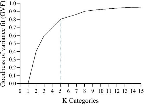
The Jenks natural breaks method calculates the sum of variances for each class, compares the classifications with the sum of variances, and the minimum value of the sum of variances is the optimal result. The K value needs to be determined before classification. If the K value is too large, it will enhance an individual's impact on the whole. If the K value is too small, the difference of interest values in different regions will be too small. Both of these situations will affect the accuracy of ϵ. Therefore, the goodness of variance fit (GVF) method is used to determine the K value. The calculation formula is as follows: $SDCM=\sum _{i=1}^k{\displaystyle \frac{1}{N_i}\sum _{i=1}^{N_i}(z_{ij}-{\overline{z}}_j{)}^2}$ (3) $\begin{array}{c}\mathrm{SDAM}={\displaystyle \frac{1}{N}\sum _{i=1}^N{(z_i-\overline{z})}^2}\end{array}$(3) $\mathrm{GVF}=1-{\displaystyle \frac{\mathrm{SDCM}}{\mathrm{SDAM}}}$

The sum of squared deviations from the array mean (SDAM) is the variance of the original data. The sum of squared deviations about class mean (SDCM) is the sum of the variances of each class. When the GVF value is closer to 1, the classification effect is better. By plotting the relationship between K and the GVF, it can be found that when K = 5, there will be a better classification effect, so ∂ is divided into five categories, as shown in Figure 4.

After all values are classified into five categories, these categories are ranked from high to low according to the average value, and each category corresponds to values of 5, 4, 3, 2 or 1. Finally, these values are added to the corresponding ϵ. As the number of scene observations increases, ϵ will more accurately reflect the interest values of different real 3D models in the scene. When the scene needs to load the model of a region, the program first retrieves the 3D grid intersecting with the viewing frustum in the scene and then renders the real 3D models where these 3D grids are located according to the distance.

Figure 4. Relationship between K and the GVF.

3.3 Viewing the frustum prediction method of virtual reality based on the Kalman filter

When the human eye observes a scene in VR, the observation region is determined by head movement and eye attention. Eye movement is discrete and jumping, which leads to difficulty and inaccuracy in eye prediction (Buettner et al. 2018). Through the method in Section 3.2, the eye observation region can be filtered, and the region with a high interest value can be loaded first. However, this loading needs to be based on the premise of predicting the user's viewing frustum in advance. It only takes approximately 200 ms for the human eye to scan the display range of a VR helmet, but it takes longer to load and draw the entire real 3D model (Albert et al. 2017).

The helmet rotation is a continuous process, so, the prediction of helmet rotation is possible and has good accuracy. This study predicts the position of the viewing frustum at the next time through the rotation data of the VR helmet in the previous period. Using the predicted viewing frustum to determine which real 3D models need to be rendered, the ROI value of these models determines the rendering order.

The continuous and relatively slow-moving speed of the head means that the next rotation of the VR helmet can be predicted. The movement of the VR helmet is determined by the position (x, y, z) and the angle (α, β, γ) in the virtual scene, where α is the angle of rotation around the x-axis, β is the angle of rotation around the y-axis, and $\gamma$ is the angle of rotation around the z-axis, and the position of the visual frustum is determined from these three angles, as shown in Figure 5.

Figure 5. Virtual reality viewing frustum.

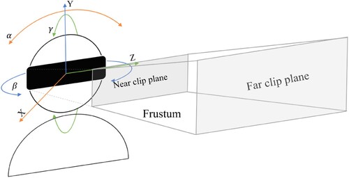
The problem of predicting the VR viewing frustum can be simplified to predict the state of the next time according to the past state through extrapolation. Extrapolation methods mainly include Lagrange interpolation, the Hermite interpolation method, and a Kalman filter. The Lagrange method is a polynomial-based method, which has less computation and is suitable for smooth motion trajectory prediction. However, when the interpolation times are high, the Runge phenomenon will appear, resulting in a large deviation of the interpolation results. Hermite interpolation is an optimization of the Lagrange interpolation method, but it requires the same derivative value at the viewpoint and has great restrictions on use, so it is not suitable for viewing frustum prediction. A Kalman filter is a linear optimal filtering algorithm (Meinhold and Singpurwalla 1983) that uses the mean square error and the criterion of the minimum mean square error to predict the rotation of the VR helmet. It has high accuracy and no requirements for the movement of the viewing frustum (Gómez and Maravall 1994). In VR, to prevent the occurrence of dizziness, teleportation movement mode is mostly used. This movement mode is discontinuous and cannot realize position prediction through extrapolation. Therefore, it is more reasonable to extrapolate and predict the rotation of the VR helmet using a Kalman filter (Zhang and Zhang 2010).

In the process of user use, the current state of the camera is recorded at a certain frame interval $f_{inr}$. Assuming that the rotation angle of the camera about the x-axe, y-axe, and z-axe at time t is $({\alpha }_t,{\beta }_t,{\gamma }_t)$, the angular velocity in the three directions is $({\omega }_{xt},{\omega }_{yt},{\omega }_{zt})$, and the state of the camera is (4) $\begin{array}{c}{x}_t={\left[\begin{array}{cccccc}{\alpha }_t& {\beta }_t& {\gamma }_t& {\omega }_{xt}& {\omega }_{yt}& {\omega }_{zt}\end{array}\right]}^T\end{array}$(4) The motion formula of the VR helmet is ${\alpha }_{t+1}={\alpha }_t+{\omega }_{xt}{f}_{inr}$ (5) $\begin{array}{c}{\beta }_{t+1}={\beta }_t+{\omega }_{yt}{f}_{inr}\end{array}$(5) ${\gamma }_{t+1}={\gamma }_t+{\omega }_{zt}{f}_{inr}$

The process noise is regarded as white noise, the value is 0, and the Kalman filter state transition matrix is (6) $\begin{array}{c}A(K|K-1)=\left[\begin{array}{cc}1& f_{inr}\\ 0& 1\end{array}\right]\end{array}$(6) To modify the VR helmet rotation state parameters, the following equation is constructed using the helmet rotation angle in the virtual scene: ${\alpha }_t=\left[\begin{array}{cc}1& 0\end{array}\right]\left[\begin{array}{c}{\alpha }_t\\ {\omega }_{xt}\end{array}\right]+U_k$ (7) $\begin{array}{c}{\beta }_t=\left[\begin{array}{cc}1& 0\end{array}\right]\left[\begin{array}{c}{\beta }_t\\ {\omega }_{yt}\end{array}\right]+U_k\end{array}$(7) ${\gamma }_t=\left[\begin{array}{cc}1& 0\end{array}\right]\left[\begin{array}{c}{\gamma }_t\\ {\omega }_{zt}\end{array}\right]+U_k$$U_k$ is the observation noise, since the observation value is obtained by reading the real-time parameters of the helmet in the scene, $U_k=0$. When $t=t_0$, the initial angle and covariance initial value of the helmet in the scene are set; when $t=t_k$, the state prediction formula of the system is (8) $\begin{array}{c}\hat{x}(k|k-1)=A(k|k-1)\hat{x}(k|k-1)\end{array}$(8) The covariance prediction formula is (9) $\begin{array}{c}P(k|k-1)=A(k|k-1)\hat{x}(k-1|k-1)+Q_t\end{array}$(9) The filter gain coefficient matrix $K_k$ is (10) $\begin{array}{c}{K}_k=P(k|k-1)H_K^T{(H_{k}P(k|k-1)H_k^T+R_k)}^{-1}\end{array}$(10) Optimal estimation of state vector (11) $\begin{array}{c}\hat{x}(k|k)=\hat{x}(k|k-1)+K_k(Z_k-H_k)\hat{x}(k-1|k-1)\end{array}$(11) The covariance updating formula of state vector is (12) $\begin{array}{c}P(k|k)=(I-K_k{H}_k)p(k|k-1)\end{array}$(12) The angle of the helmet after the current frame interval is predicted according to the state prediction formula of the system, and the angle variation range of the camera is set to 0° to 360°. When the predicted angle of the helmet is obtained, the range of the viewing frustum is calculated according to the predicted angle and other parameters of the helmet, and the real 3D model outside the viewing frustum is culled. Since the size of the real 3D model is not constant, the model that intersects with the visual frustum is taken as the model to be rendered. After the model to be rendered is obtained, the model to be rendered preferentially is determined according to the ϵ value of the ROI within the visual frustum. For data calls of different levels of detail, the method of selecting calls according to distance is adopted, as shown in Formula 13. (13) $\begin{array}{c}\{\begin{array}{c}\begin{array}{c}Lo{d}_1,0<d\le D_1\\ Lo{d}_2,D_1<d\le D_2\\ \dots \end{array}\\ Lo{d}_n,D_{n-1}<d\le D_n\end{array}\end{array}$(13) where $Lo{d}_n$ is the nth level of the model, $d$is the distance from the camera to the center point of the model at this time, and $D_n$ is the distance range.

4 Experiment and analysis

4.1 Experimental design and case region

This study selected a case region for the experiment and evaluated the correctness of the research method from the perspectives of scene rendering efficiency and user experience. 46 testers were invited to participate in the experiment, ranging in age from 22 to 31, including undergraduate, graduate and doctoral students with GIS professional backgrounds. The participants were randomly divided into two groups, an experimental group and a control group, with 23 people in each group. The experimental group used the method proposed in this study to collect their ROIs and predict the rotation of the VR helmet, while the control group used the normal scene rendering method. Before the experiment, training was conducted on the use of the VR equipment to avoid deviation caused by different proficiency in the use of the equipment. The experiment lasted approximately 151 s, and a virtual avatar of the tester moved along a preset route with a speed of 10 m/s in the scene, with a distance of approximately 1500 m. To avoid dizziness caused by fast moving speed, the height of the virtual avatar was set to 10–20 m from the ground, and participants could freely rotate their heads during the process. During the test, the ROIs of the experimental group were collected through VR eye-tracking equipment.

An area of 4.2 km² of UAV oblique photographic data in Luding County, Sichuan Province, China was selected as the topographic experimental area. The total size of the real 3D model data is 233.9 GB (Gigabyte), and each real 3D model has five levels of detail, including buildings, rivers, hills and other elements in the area. The data size of the mountainous area is approximately 108.4 GB, and the data size of the building area is approximately 125.5 GB These data are stored in folders in the form of files, but their index data are stored in the MySQL database (Figure 6). The proportion of levels of detail (LODs) is shown in Table 1.

Figure 6. Experimental region.

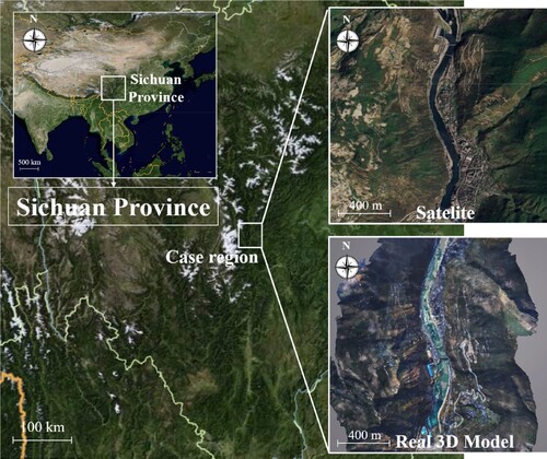
Table 1. Data size and distribution.

	LOD0	LOD1	LOD2	LOD3	LOD4	Total
Building area	3.9%	10.1%	18.8%	27.3%	39.8%	100% (125.5GB)
Mountain area	4.1%	11.8%	18.4%	26.3%	39.4%	100% (108.4GB)

The equipment used in the experiment is shown in Table 2.

Table 2. System development environment configuration.

Equipment and software	Environment configuration	Detailed information
Hardware	Central processing unit(CPU)	Intel i7-10870
	Memory	32 GB
	GPU	NVIDIA RTX 3080
	Video memory	16 GB
	VR equipment	HTC VIVE
	Eye tracking accessory	Droolon F1
Software	System	Windows 10
	Software	Unity 3D 2020.3.8 Steam VR Visual Studio 2019

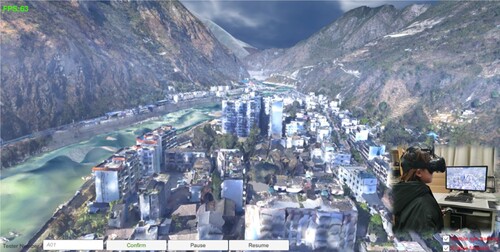
Using the above data and equipment, we developed a prototype system for testing, as shown in Figure 7.

Figure 7. Main interface of the prototype system.

4.2 Experimental results and analysis

4.2.1 Scene rendering efficiency results and analysis

Scene rendering efficiency can be measured by the rendering frame rate and the user ROI accuracy rate. The rendering frame rate directly determines the experience of users in a VR scene. When a user browses a scene, the system records the current VR scene rendering frame rate and the number of triangles rendered in the scene per second and then calculates the average frame rate of all people at each moment. The experimental result is shown in Figure 8.

Figure 8. Average rendered frame rate and number of triangles in the scene.

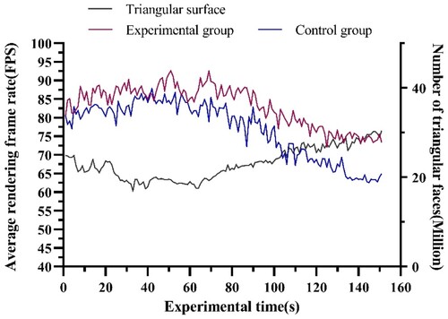
The average frame rate of the experimental group during the whole test was 83.16 frames per second (FPS) and that of the control group was 76.82 FPS. Compared with that of the control group, the rendering efficiency of the experimental group increased by approximately 8.2%. We used Mann–Whitney U test to compare whether there were differences between the two groups ($\alpha =0.05$). The difference of frame rate between the experimental group and the control group was statistically significant (p = 0.00**). In addition, the standard deviation of the experimental group was 5.43 and that of the control group was 7.59, showing that the frame rate stability of the experimental group was better than that of the control group. The view prediction allows the computer to spend less time retrieving and loading data, thus achieving an increase in frame rate. When the viewing frustum moves to the predicted position, the real 3D model that has been loaded into main memory and video memory can be quickly rendered.

Different from the mountain data in the early part of the experiment, the latter part of the data was mainly buildings, which had more vertices and triangles in the same region, resulting in a decrease in rendering frame rate for both the experimental and control groups after 70 s. However, this downward trend was more moderate in the experimental group because the rendering method of the experimental group makes the utilization of the CPU and GPU more balanced. According to the Pearson correlation coefficient calculation method, the correlation coefficient $R^2$between the frame rate and the number of triangles in the experimental group was −0.89 (p < 0.01) and that in the control group was −0.91 (p < 0.01), which shows that the rendering frame rate is negatively correlated with the number of triangles, and the GPU of the experimental group can work more efficiently.

To show the ROI recognition accuracy of the experimental group, the interest value ${\epsilon }_n$ of each real 3D model was recorded before the test, and the interest degree ${\epsilon }_n^{{}^{\mathrm{\prime }}}$ of each real 3D model was recorded during the experiment according to the method in Section 2.2, where n represents the nth real 3D model. After the test, Formula 14 was used to calculate the sum $\rho$ of the difference in the interest between an individual and the group for each real 3D model. (14) $\begin{array}{c}\rho =\sum _1^n\left|{\displaystyle \frac{{\epsilon }_n}{{\sum }_n^{\epsilon }}-{\displaystyle \frac{{{\epsilon }^{\mathrm{\prime }}}_n}{{\sum }_n^{{\epsilon }^{\mathrm{\prime }}}}}}\right|\end{array}$(14) Although the observation path of different testers was the same, and they were not allowed to move freely, the observation preference of different testers may lead to a situation where some regions are not observed, which will lead to the incomparability of $\rho$ values. In view of this situation, this study selected a real 3D model observed by all the testers for analysis and comparison. The experimental group results are shown in Figure 9.

Figure 9. Relationship between the number of testers and the ρ value.

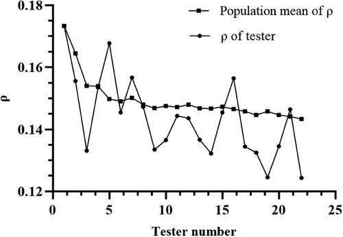
The results show that as the number of testers increases, the accuracy of the ROI gradually increases. When ρ is equal to approximately 0.145, the increase in the number of testers no longer improves the accuracy significantly, which means that the ROIs of the testers in the scene are mostly the same. Therefore, it is feasible to improve the visual experience of testers by prioritizing the rendering of ROIs. The accuracy of the viewing frustum prediction based on the Kalman filter remains at approximately 87%. By analyzing user behavior data in the virtual scene, it can be found that the reason for this phenomenon is users’ sudden turn of the helmet, which is difficult to predict. This sudden turn is random, and it is difficult to predict and avoid. With the increase in frame rate and the decrease in Kalman filter calculation interval, the prediction accuracy can be further improved. In addition, we compared the speed of eye tracking while directly rendering the real 3D model with that of frustum preloading. The initial position and angle of the HMD in the virtual scene of the two groups remain the same. The most detailed model is rendered in the ROI, and the rendering methods of other regions are based on Formula 13. There were 26 participants in the experiment, 13 in each group. Due to the randomness of users’ observation habits, we added graphical symbols to guide users to observe the specified area. The data size of the test area is approximately 381 MB (MByte) (Figure 10).

Figure 10. Direction guide symbol and test region.

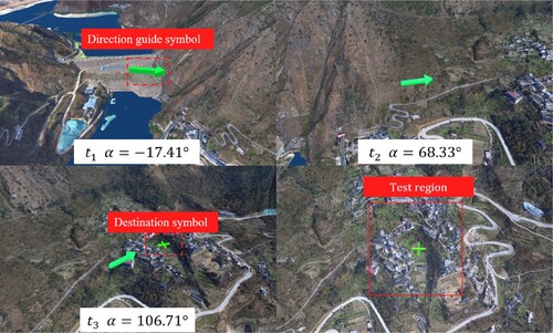
The initial angle of the HMD in the x–z plane is approximately −17.41°, and the test region can be observed only after rotating approximately 120°, which takes approximately 3–5 s. In the experimental group, when the tester moves the HMD, the time it takes from the intersection of the predicted frustum and the test region to the completion of the real 3D model rendering of the test region (Group A) was recorded, as well as the time it takes from the intersection of the tester's eye attention region and the test region to the completion of model rendering (Group B). In the control group, the time it takes from the intersection of the eye focus region of the tester with the test region to the completion of the rendering of the real 3D model was recorded (Group C). We used the Kolmogorov–Smirnov test to test the normality of these groups, and the results are shown in Table 3.

Table 3. Tests of normality.

	Kolmogorov–Smirnov test
	Statistic	df	Sig.
Group A	0.172	13	.200*
Group B	0.093	13	.200*
Group C	0.143	13	.200*

The time consumption of Group A was 338.92 ± 15.06 ms, and that of Group C was 339.77 ± 15.17 ms. There was no significant difference between the two groups (P > 0.05). This occurred because no matter which method was adopted, the computer took the same time to load the data. There is a significant difference (p = 0.00**) between Group B (113.23 ± 13.27 ms) and Group C. Compared with Group C, Group B takes 67% less time, which means that this method can predict the user frustum location approximately 200 ms before Group C. Note that times of Group B and Group C are the actual waiting times of users in virtual reality, so the two groups of data are comparable.

4.2.2 User experience results and analysis

The users filled out a questionnaire immediately after the test. For the experience in VR scenes, the commonly used evaluation indicators include the effectiveness, efficiency and satisfaction (Fu et al. 2021). Effectiveness refers to whether the adopted visualization methods will bring differences in visual perception. Therefore, to verify the effectiveness of the method proposed in this study combined with the characteristics of real 3D scenes, this study designed three questions to evaluate user experience during browsing. The questionnaire as shown in Table 4, then the reliability and validity of the questionnaire are tested (Li et al. 2021).

Table 4. Questions on the questionnaire.

No.	Scoring items	Score
Q1	Did you feel motion sickness during the experiment?	1. No 2. Mildly 3. Moderately 4. Strongly 5. Intensely
Q2	Do you feel stuck or delayed when switching real 3D models with different level of details?	1. No 2. Feel a little 3. Occasionally feel 4. Feel distinctly 5. Strongly
Q3	Did you feel smooth browsing in the VR 3D scene?	1. Very smooth 2. Smooth 3. Neutral 4. Rough 5. Very rough

As shown in the Table 4, five options were set for each question, representing 1–5 points. The total score of the three scoring items was the total score of each tester. The lower the overall score is, the better the experience effect is, and the higher the score is, the worse the experience effect is.

Whether it is to improve the rendering frame rate or to predict the ROI more accurately, the ultimate purpose is to provide VR users with a better visual experience, so users’ feelings can directly reflect whether the method in this study is effective. Both the experimental group and the control group received questionnaires after the test, and a total of 46 valid data points were received, 23 for each group. After verification, there were 23 valid questionnaires in the experimental group and 22 valid questionnaires in the control group. The invalid questionnaire was due to conflicting scores for different questions. The valid questionnaire results are shown in Table 5 and Table 6.

Table 5. Reliability and validity test results.

		Bartlett’s test
Cronbach’s $\alpha$ value	KMO value	Approx. chi-square	df	Sig.
0.969	0.871	168.803	15	0.000**

Table 6. Questionnaire results.

Question	Group	Mean	P
Q1	Experimental group	1.87 ± 0.76	0.0457
	Control group	2.50 ± 1.01
Q2	Experimental group	1.96 ± 0.71	0.0013
	Control group	2.86 ± 1.04
Q3	Experimental group	1.73 ± 0.69	0.0343
	Control group	2. 27 ± 0.94

The distribution of the questionnaire results is shown in Figure 11.

Figure 11. Distribution of testers’ scores.

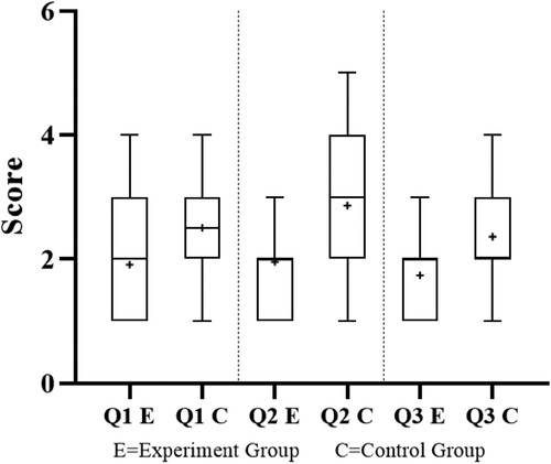
Overall, the average scores of the three questions in the experimental group were lower than those in the control group. The Q1, Q2, and Q3 scores decreased by approximately 25.2%, 31.5% and 23.8%, respectively. In particular, the testers’ feelings of switching between different LOD of real 3D models decreased.

As seen from the Q1 results, the incidence probability of motion sickness in the experimental group is significantly lower than that in the control group, and dizziness has lower likelihood of occurrence when the VR scene has a higher frame rate. Sometimes motion sickness still occurs when the average frame rate is high. This is because in VR, especially in scenes with high triangular density, the computer cannot render the moving images quickly due to the sudden movement or turning of the user, resulting in frames becoming stuck or tearing, which is called frame loss. In this study, the turns of the testers in the experimental group were predicted, which made the rendering region and rendering order deterministic and reduced the computational pressure on the GPU and CPU caused by the turning of the helmet. This also enabled the images to be rendered more quickly after turning, thereby avoiding the dizziness caused by frame loss and improving the experience of the VR users. In this experiment, it can be observed that the increase in frame rate is 8.2%, and the probability of motion sickness is obviously reduced by 54.5% in the experimental group (Q2 Score > 2), which further verifies that the frame loss reduction is helpful to improve the experience of VR users.

For Q2, the result of the experimental group was significantly better than that of the control group (p = 0.0013) due to the prediction of the tester's viewing frustum and the rendering of the real 3D model of interest within the viewing frustum in advance. Meanwhile, we also observed that when the change in the tester's view field was small, the tester had a strong feeling of LOD switching. This is because when the change of view field is small, the predicted result is the same as that of the previous time, which cannot bring the preload effect to the tester and inevitably brings the feeling of LOD switching. For Q3, the fluency felt by the experimental group was better than that of the control group, and the difference was statistically significant (p = 0.0343). The improvement of the frame rate and stability together bring about the improvement in fluency, thus comprehensively improving the experience of the testers.

5. Discussion

5.1 General discussion

Real 3D model is an important technology in building digital earth. At the same time, using real 3D scene in virtual reality is an effective method to effectively improve the immersion and realism of virtual reality. Especially with the development of UAV technology, the data volume and precision of real three-dimensional model are gradually improved. The existing scene optimization methods can not render and use these data efficiently in virtual reality. Because these methods pay more attention to how to optimize the computer hardware, and do not take into account the special interaction methods of virtual reality and the characteristics of human eyes when observing the scene. Moreover, the response speed of the existing eye tracking rendering methods can not satisfy the efficient rendering of the real 3D model in virtual reality, resulting in the reduction of VR user experience and limiting the reference of the real 3D model in virtual reality. Our method obtains the ROI of each user through eye tracking equipment, and gives rendering priority to each real 3D model. Then, the rotation angle of HMD is predicted by Kalman filter to obtain viewing frustum, which is preloaded and rendered according to the priority of the real three-dimensional model in viewing frustum. Finally, we verify our method by constructing a prototype system. Kalman filter can predict the visual cone with an accuracy of about 87%, and the frame rate of real 3D scene in virtual reality can be improved by 8.3%.

5.2 Practical implication

In recent years, great progress has been made in the acquisition and processing technology of real 3D models (Liénard et al. 2016; Ji and Luo 2019), but their application is more difficult due to the large amount of data and complex data structure of real 3D models. Especially in virtual reality, researchers rarely build virtual geographic scenes through real three-dimensional models, and they use DEM data instead (Fu et al. 2021). The key problem is that virtual reality has higher requirements for scene rendering, and there is a trade-off between performance and visual quality. Our research aims to improve this problem through eye-tracking equipment because people's regions of interest in the same scene are often similar (Cheng, Chu, and Wu 2005). Through the enhancement in the rendering of the area observed by human eyes, we can effectively reduce the dependence on hardware and make the use of hardware resources more reasonable. With the same computing performance, virtual reality scenes can provide users with a better visual experience, greatly reduce the occurrence of motion sickness, expand the application scope and platform of real three-dimensional models, and have positive significance for the construction of digital earth.

6 Conclusion and future work

This research adopts the method of combining ROI recognition and viewing frustum prediction to optimize the rendering of real 3D scene in virtual reality, and analyzes the effectiveness of this method through experiments. According to our results, the rendering order of the real 3D model determined according to the ROI is helpful to improve the user experience. Under the same computer performance, the user's visual fluency of the virtual scene is improved. Kalman filtering can predict the motion trajectory of virtual reality HMD, which is very important for preloading the real three-dimensional model contained in viewing frustum at the next time. Led to VR scenes rarely exhibit picture stutter and tear, and greatly reduced the user's motion sickness. Although the above research has made some progress, there are still some shortcomings. For example, in our research, the rendering order of the real 3D model is based on the previous user’s regions of interest. The premise of this method is that the user has similar regions of interest. In future work, we may try to use the current user's behavior data to amend the regions of interest in real time. Moreover, Kalman filtering is not good at predicting the sudden turn of an HMD. In fact, the current algorithm has difficulty identifying this behavior because this behavior is accidental, and there are great differences between individuals. Perhaps the use of neural networks and a large number of training samples can improve this situation.

Author contributions

Conceptualization, Jun Zhu; Methodology, Pei Dang; Resources, Jigang You, Yiqun Shi and Yuhang Gong; Software, Pei Dang and Jianlin Wu; Validation, Jun Zhu, Weilian Li; Writing – original draft, Pei Dang; Writing – review & editing, Jun Zhu and Lin Fu. All authors have read and agreed to the published version of the manuscript.

Disclosure statement

No potential conflict of interest was reported by the author(s).

Data availability statement

The data that support the findings of this study are available from the corresponding author, Zhu, upon reasonable request.

Additional information

Funding

This research was supported by the National Natural Science Foundation of China (grant numbers U2034202; 41871289; 42171397), the Sichuan Science and Technology Program (grant number 2020JDTD0003).

References

- Albert, R., A. Patney, D. Luebke, and J. Kim. 2017. “Latency Requirements for Foveated Rendering in Virtual Reality.” ACM Transactions on Applied Perception (TAP) 14 (4): 1–13. doi:10.1145/3127589.
- Alizadehsalehi, S., A. Hadavi, and J. C. Huang. 2020. “From BIM to Extended Reality in AEC Industry.” Automation in Construction 116: 103254. doi:10.1016/fj.autcon.2020.103254
- Asgharian, L., and H. Ebrahimnezhad. 2020. “How Many Sample Points are Sufficient for 3D Model Surface Representation and Accurate Mesh Simplification?” Multimedia Tools and Applications 79 (39): 29595–29620. doi:10.1007/s11042-020-09395-3.
- Atchison, D. A., and L. N. Thibos. 2016. “Optical Models of the Human eye.” Clinical and Experimental Optometry 99 (2): 99–106. doi:10.1111/cxo.12352.
- Baloh, R. W., H. R. Konrad, A. W. Sills, and V. Honrubia. 1975. “The Saccade Velocity Test.” Neurology 25 (11): 1071–1071. doi:10.1212/wnl.
- Billen, M. I., O. Kreylos, B. Hamann, M. A. Jadamec, L. H. Kellogg, O. Staadt, and D. Y. Sumner. 2008. “A Geoscience Perspective on Immersive 3D Gridded Data Visualization.” Computers & Geosciences 34 (9): 1056–1072. doi:10.1016/j.cageo.2007.11.009.
- Cabiddu, D., and M. Attene. 2015. “Large Mesh Simplification for Distributed Environments.” Computers & Graphics 51: 81–89. doi:10.1016/j.cag.2015.05.015.
- Buettner, R., S. Sauer, C. Maier, and A. Eckhardt. 2018. “Real-time Prediction of User Performance Based on Pupillary Assessment via Eye Tracking.” AIS Transactions on Human-Computer Interaction 10 (1): 26–56. doi:10.17705/1thci.00103.
- Cai, Z., C. Fang, Q. Zhang, and F. Chen. 2021. “Joint Development of Cultural Heritage Protection and Tourism: The Case of Mount Lushan Cultural Landscape Heritage Site.” Heritage Science 9 (1): 1–16. doi:10.1186/s40494-021-00558-5.
- Campomanes-Álvarez, B. R., O. Cordon, and S. Damas. 2013. “Evolutionary Multi-objective Optimization for Mesh Simplification of 3D Open Models.” Integrated Computer-Aided Engineering 20 (4): 375–390. doi:10.3233/ICA-130443.
- Chang, E., H. T. Kim, and B. Yoo. 2020. “Virtual Reality Sickness: A Review of Causes and Measurements.” International Journal of Human–Computer Interaction 36 (17): 1658–1682. doi:10.1080/10447318.2020.1778351.
- Checa, D., and A. Bustillo. 2020. “A Review of Immersive Virtual Reality Serious Games to Enhance Learning and Training.” Multimedia Tools and Applications 79 (9): 5501–5527. doi:10.1007/s11042-019-08348-9.
- Chen, M., H. Lin, M. Hu, L. He, and C. Zhang. 2013. “Real-geographic-scenario-based Virtual Social Environments: Integrating Geography with Social Research.” Environment and Planning B: Planning and Design 40 (6): 1103–1121. doi:10.1068/b38160.
- Cheng, W. H., W. T. Chu, and J. L. Wu. 2005. “A Visual Attention Based Region-of-Interest Determination Framework for Video Sequences.” IEICE Transactions on Information and Systems 88 (7): 1578–1586. doi:10.1093/ietisy/e88-d.7.1578.
- Clay, V., P. König, and S. Koenig. 2019. “Eye Tracking in Virtual Reality.” Journal of Eye Movement Research 12: 1. doi:10.16910/jemr.12.1.3.
- Dang, P., J. Zhu, S. Pirasteh, W. Li, J. You, B. Xu, and C. Liang. 2021. “A Chain Navigation Grid Based on Cellular Automata for Large-scale Crowd Evacuation in Virtual Reality.” International Journal of Applied Earth Observation and Geoinformation 103: 102507. doi:10.1016/j.jag.2021.102507.
- Deubel, H., and W. X. Schneider. 1996. “Saccade Target Selection and Object Recognition: Evidence for a Common Attentional Mechanism.” Vision Research 36 (12): 1827–1837. doi:10.1016/0042-6989(95)00294-4.
- Duchowski, A. T., and A. Çöltekin. 2007. “Foveated Gaze-Contingent Displays for Peripheral LOD Management, 3D Visualization, and Stereo Imaging.” ACM Transactions on Multimedia Computing, Communications, and Applications (TOMM) 3 (4): 1–18. doi:10.1145/1314303.1314309.
- Dwyer, R. A. 1987. “A Faster Divide-and-Conquer Algorithm for Constructing Delaunay Triangulations.” Algorithmica 2 (1): 137–151. doi:10.1007/BF01840356.
- Findlay, J. M. 1997. “Saccade Target Selection During Visual Search.” Vision Research 37 (5): 617–631. doi:10.1016/S0042-6989(96)00218-0.
- Fortune, S. 1987. “A Sweepline Algorithm for Voronoi Diagrams.” Algorithmica 2 (1): 153–174. doi:10.1007/BF01840357.
- Fu, L., J. Zhu, W. Li, Q. Zhu, B. Xu, Y. Xie, Y. Zhang, et al. 2021. “Tunnel Vision Optimization Method for VR Flood Scenes Based on Gaussian Blur.” International Journal of Digital Earth 14 (7): 821–835. doi:10.1080/17538947.2021.1886359.
- Gómez, V., and A. Maravall. 1994. “Estimation, Prediction, and Interpolation for Nonstationary Series with the Kalman Filter.” Journal of the American Statistical Association 89 (426): 611–624. doi:10.1080/01621459.1994.10476786.
- Ho, H. F. 2014. “The Effects of Controlling Visual Attention to Handbags for Women in Online Shops: Evidence from Eye Movements.” Computers in Human Behavior 30: 146–152. doi:10.1016/j.chb.2013.08.006.
- Hu, Y., J. Zhu, W. Li, Y. Zhang, Q. Zhu, H. Qi, H. Zhang, Z. Cao, W. Yang, and P. Zhang. 2018. “Construction and Optimization of Three-dimensional Disaster Scenes Within Mobile Virtual Reality.” ISPRS International Journal of Geo-Information 7 (6): 215. doi:10.3390/ijgi7060215.
- Huang, W., J. Chen, and M. Zhou. 2020. “A Binocular Parallel Rendering Method for VR Globes.” International Journal of Digital Earth 13 (9): 998–1016. doi:10.1080/17538947.2019.1620883.
- Ji, H., and X. Luo. 2019. “3D Scene Reconstruction of Landslide Topography Based on Data Fusion Between Laser Point Cloud and UAV Image.” Environmental Earth Sciences 78 (17): 1–12. doi:10.1007/s12665-019-8516-5.
- Kim, H. K., J. Park, Y. Choi, and M. Choe. 2018. “Virtual Reality Sickness Questionnaire (VRSQ): Motion Sickness Measurement Index in a Virtual Reality Environment.” Applied Ergonomics 69: 66–73. doi:10.1016/j.apergo.2017.12.016.
- Konrad, R., A. Angelopoulos, and G. Wetzstein. 2020. “Gaze-contingent Ocular Parallax Rendering for Virtual Reality.” ACM Transactions on Graphics (TOG) 39 (2): 1–12. doi:10.1145/3361330.
- Lee, D. T., and B. J. Schachter. 1980. “Two Algorithms for Constructing a Delaunay Triangulation.” International Journal of Computer & Information Sciences 9 (3): 219–242. doi:10.1007/BF00977785.
- Lee, J. H., I. Yanusik, Y. Choi, B. Kang, C. Hwang, J. Park, D. Nam, and S. Hong. 2020. “Automotive Augmented Reality 3D Head-up Display Based on Light-Field Rendering with Eye-Tracking.” Optics Express 28 (20): 29788–29804. doi:10.1364/OE.404318.
- Li, J., Y. Yao, P. Duan, Y. Chen, S. Li, and C. Zhang. 2018a. “Studies on Three-Dimensional (3D) Modeling of UAV Oblique Imagery with the Aid of Loop-Shooting.” ISPRS International Journal of Geo-Information 7 (9): 356. doi:10.3390/ijgi7090356.
- Li, X., W. Yi, H. L. Chi, X. Wang, and A. P. Chan. 2018b. “A Critical Review of Virtual and Augmented Reality (VR/AR) Applications in Construction Safety.” Automation in Construction 86: 150–162. doi:10.1016/j.autcon.2017.11.003.
- Li, W., J. Zhu, L. Fu, Q. Zhu, Y. Xie, and Y. Hu. 2021. “An Augmented Representation Method of Debris Flow Scenes to Improve Public Perception.” International Journal of Geographical Information Science 35 (8): 1521–1544. doi:10.1080/13658816.2020.1833016.
- Liang, Y., F. He, and X. Zeng. 2020. “3D Mesh Simplification with Feature Preservation Based on Whale Optimization Algorithm and Differential Evolution.” Integrated Computer-Aided Engineering 27 (4): 417–435. doi:10.3233/ICA-200641.
- Liénard, J., A. Vogs, D. Gatziolis, and N. Strigul. 2016. “Embedded, Real-time UAV Control for Improved, Image-based 3D Scene Reconstruction.” Measurement 81: 264–269. doi:10.1016/j.measurement.2015.12.014.
- Lin, H., M. Chen, and G. Lu. 2013. “Virtual Geographic Environment: A Workspace for Computer-Aided Geographic Experiments.” Annals of the Association of American Geographers 103 (3): 465–482. doi:10.1080/00045608.2012.689234.
- Lin, Y., M. Jiang, Y. Yao, L. Zhang, and J. Lin. 2015. “Use of UAV Oblique Imaging for the Detection of Individual Trees in Residential Environments.” Urban Forestry & Urban Greening 14 (2): 404–412. doi:10.1016/j.ufug.2015.03.003.
- Lin, M., F. Y. Li, and H. Zhou. 2020. “A Research on the Combination of Oblique Photography and Mobile Applications Based on the Sustainable Development of Tourism.” Sustainability 12 (9): 3501. doi:10.3390/su12093501.
- Lingas, A. 1986. “The Greedy and Delauney Triangulations are not Bad in the Average Case.” Information Processing Letters 22 (1): 25–31. doi:10.1016/0020-0190(86)90038-4.
- Lingua, A., F. Noardo, A. Spanò, S. Sanna, and F. Matrone. 2017. “3D Model Generation Using Oblique Images Acquired by UAV.” The International Archives of the Photogrammetry, Remote Sensing and Spatial Information Sciences 42 (4): 107–115. doi:10.5194/isprs-archives-XLII-4-W2-107-2017.
- Meinhold, R. J., and N. D. Singpurwalla. 1983. “Understanding the Kalman Filter.” The American Statistician 37 (2): 123–127. doi:10.1080/00031305.1983.10482723.
- Meng, X., R. Du, and A. Varshney. 2020. “Eye-dominance-guided Foveated Rendering.” IEEE Transactions on Visualization and Computer Graphics 26 (5): 1972–1980. doi:10.1109/TVCG.2020.2973442.
- Patney, A., M. Salvi, J. Kim, A. Kaplanyan, C. Wyman, N. Benty, D. Luebke, and A. Lefohn. 2016. “Towards Foveated Rendering for Gaze-Tracked Virtual Reality.” ACM Transactions on Graphics (TOG) 35 (6): 1–12. doi:10.1145/2980179.2980246.
- Purucker, C., J. R. Landwehr, D. E. Sprott, and A. Herrmann. 2013. “Clustered Insights: Improving Eye Tracking Data Analysis Using Scan Statistics.” International Journal of Market Research 55 (1): 105–130. doi:10.2501/IJMR-2013-009.
- Sibson, R. 1978. “Locally Equiangular Triangulations.” The Computer Journal 21 (3): 243–245. doi:10.1093/comjnl/21.3.243.
- Stein, B. E., N. London, L. K. Wilkinson, and D. D. Price. 1996. “Enhancement of Perceived Visual Intensity by Auditory Stimuli: A Psychophysical Analysis.” Journal of Cognitive Neuroscience 8 (6): 497–506. doi:10.1162/jocn.1996.8.6.497.
- Stein, N., D. C. Niehorster, T. Watson, F. Steinicke, K. Rifai, S. Wahl, and M. Lappe. 2021. “A Comparison of eye Tracking Latencies among Several Commercial Head-Mounted Displays.” i-Perception 12 (1): 2041669520983338. doi:10.1177/2041669520983338.
- Su, P., and R. L. S. Drysdale. 1997. “A Comparison of Sequential Delaunay Triangulation Algorithms.” Computational Geometry 7 (5-6): 361–385. doi:10.1016/S0925-7721(96)00025-9.
- Sun, G., J. Zhang, K. Zheng, and X. Fu. 2020. “Eye Tracking and Roi Detection Within a Computer Screen Using a Monocular Camera.” Journal of Web Engineering 19 (7-8): 1117–1146. doi:10.13052/jwe1540-9589.19789.
- Tibaldi, A., F. L. Bonali, F. Vitello, E. Delage, P. Nomikou, V. Antoniou, U. Becciani, B. Van Wyk de Vries, M. Krokos, and M. and Whitworth. 2020. “Real World–Based Immersive Virtual Reality for Research, Teaching and Communication in Volcanology.” Bulletin of Volcanology 82 (5): 1–12. doi:10.1007/s00445-020-01376-6.
- Van, J., P. Shi, and D. Zhang. 2004. “Mesh Simplification with Hierarchical Shape Analysis and Iterative Edge Contraction.” IEEE Transactions on Visualization and Computer Graphics 10 (2): 142–151. doi:10.1109/TVCG.2004.1260766.
- Verhoeven, G. 2011. “Taking Computer Vision Aloft–Archaeological Three-dimensional Reconstructions from Aerial Photographs with Photoscan.” Archaeological Prospection 18 (1): 67–73. doi:10.1002/arp.399.
- Vignais, N., R. Kulpa, S. Brault, D. Presse, and B. Bideau. 2015. “Which Technology to Investigate Visual Perception in Sport: Video vs. Virtual Reality.” Human Movement Science 39: 12–26. doi:10.1016/j.humov.2014.10.006.
- Wang, J., L. Wang, M. Jia, Z. He, and L. Bi. 2020. “Construction and Optimization Method of the Open-pit Mine DEM Based on the Oblique Photogrammetry Generated DSM.” Measurement 152: 107322. doi:10.1016/j.measurement.2019.107322.
- Wooding, D. S. 2002. “Eye Movements of Large Populations: II. Deriving Regions of Interest, Coverage, and Similarity Using Fixation Maps.” Behavior Research Methods, Instruments, & Computers 34 (4): 518–528. doi:10.3758/BF03195481.
- Xu, Y., J. Zhang, H. Zhao, C. Chen, and W. Mao. 2021. “Research on Quality Framework of Real Scene 3d Model Based on Oblique Photogrammetry.” The International Archives of Photogrammetry, Remote Sensing and Spatial Information Sciences 43: 791–796. doi:10.5194/isprs-archives-XLIII-B3-2021-791-2021.
- Yijing, W., and C. Yuning. 2018. “Construction and Analysis of 3D Scene Model of Landscape Space Based on UAV Oblique Photography and 3D Laser Scanner.” Journal of Digital Landscape Architecture 3: 283–290. doi:10.14627/537642030.
- Zhang, L., C. Han, L. Zhang, X. Zhang, and J. Li. 2014. “Web-based Visualization of Large 3D Urban Building Models.” International Journal of Digital Earth 7 (1): 53–67. doi:10.1080/17538947.2012.667159.
- Zhang, R., H. Li, K. Duan, S. You, K. Liu, F. Wang, and Y. Hu. 2020. “Automatic Detection of Earthquake-Damaged Buildings by Integrating UAV Oblique Photography and Infrared Thermal Imaging.” Remote Sensing 12 (16): 2621–2648. doi:10.3390/rs12162621.
- Zhang, L., J. She, J. Tan, B. Wang, and Y. Sun. 2019. “A Multilevel Terrain Rendering Method Based on Dynamic Stitching Strips.” ISPRS International Journal of Geo-Information 8 (6): 255–277. doi:10.3390/ijgi8060255.
- Zhang, L., P. Wang, C. Huang, B. Ai, and W. Feng. 2021. “A Method of Optimizing Terrain Rendering Using Digital Terrain Analysis.” ISPRS International Journal of Geo-Information 10 (10): 666. doi:10.3390/ijgi10100666.
- Zhang, Z., and J. Zhang. 2010. “A new Real-Time eye Tracking Based on Nonlinear Unscented Kalman Filter for Monitoring Driver Fatigue.” Journal of Control Theory and Applications 8 (2): 181–188. doi:10.1007/s11768-010-8043-0.
- Zhou, T., L. Lv, J. Liu, and J. Wan. 2021. “Application of Uav Oblique Photography in Real Scene 3d Modeling.” The International Archives of Photogrammetry, Remote Sensing and Spatial Information Sciences 43: 413–418. doi:10.5194/isprs-archives-XLIII-B2-2021-413-2021.