Landform classification based on landform geospatial structure – a case study on Loess Plateau of China

ABSTRACT

Landform classification, which is a key topic of geography, is of great significance to a wide range of fields including human construction, geological structure research, environmental governance, etc. Previous studies of landform classification generally paid attention to the topographic or texture information, whilst the watershed spatial structure has not been used. This study developed a new landform classification method based on watershed geospatial structure. Via abstracting the landform into the internal and marginal structure, we adopted the gully weighted complex network (GWCN) and watershed boundary profile (WBP) to simulate the watershed geospatial structure. Introducing various indices to quantitatively depict the watershed geospatial structure, we conducted the landform classification on the Northern Shaanxi of Loess Plateau with a watershed-based strategy and established the classification map. The classified landform distribution has significant spatial aggregation and clear regional boundaries. Classification accuracy reached 89% and the kappa coefficient reached 0.87%. Besides, the proposed method has a positive response to some similar and complex landforms. In general, the present study first utilized the watershed geospatial structure to conduct landform classification and is an efficient landform classification method with well accuracy and universality, offering additional insights for landform classification and mapping.

KEYWORDS:

• DEM
• landform classification
• geomorphological mapping
• watershed geospatial structure
• complex network

1. Introduction

Landform, as one of the most important components of the physical geography environment (Summerfield 2014), is the core content of geographical research (Xiong et al. 2021). Each landform implies a great deal of geoinformation about the natural environment, ecological resources, and human activities (Du et al. 2019). Diverse landform types formed the earth's surface under inner forces including hydrological, geological, and ecological forces (Evans 2012; Kilic Gul 2018; Moreno et al. 2004). Landform classification, which identifies and divides the earth's surface into different landform types, forms the basis and is the first step in the geomorphological mapping (Mokarram and Sathyamoorthy 2018). It is of great importance for understanding the geomorphological forming process (Hiller and Smith 2008), revealing the landform evolution mechanism (Li et al. 2020b), establishing ecological modeling (Xiong et al. 2018), and accelerating the advance of various related geoscience fields including hydrology (Lee et al. 2009), biology (O'Neill et al. 1997), geology (Du et al. 2019; Zhou et al. 2010), etc. Landform classification, therefore, has become a significant theme and attracted worldwide attention for decades in the geoscience field and earth-related disciplines (Saadat et al. 2008; Schillaci and Braun 2015; Tang et al. 2021).

Traditional landform classification and mapping mainly adopted field investigation combing with the manual interpretation of topographic maps and aerophoto (Hammond 1964; Prima et al. 2006; Saadat et al. 2008), which depends heavily on the qualitative and subjective expert experience (Mokarram and Sathyamoorthy 2018). Besides, field investigations and manual recognition unavoidably bring onerous work that is time-consuming and labor-intensive (Strahler 1956). Simultaneously, for the topographic maps or aerial photographs, the limited terrain information and morphological information fail to classify the actual complex landforms accurately (Kramm et al. 2017). In recent years, benefiting from the acquisition of different data sources such as the digital elevation model (DEM), traditional methods have been gradually substituted by different automated methodologies, especially the digital landform classification techniques (Drăguţ and Eisank 2012). With the development of DEM data acquisition, landform classification using DEM become a main technique and hotpoint in landform classification since its high accuracy and reasonable classification scheme (Xiong et al. 2018).

So far, there are two main categories of DEM-based landform classification approaches in existing research: object and pix-based approaches (Li et al. 2020b). The pixel-based approach primarily uses terrain derivatives based on pix units to quantify the terrain features, thereby revealing regional differences between different landforms (MacMillan, Jones, and McNabb 2004). Nevertheless, for the complex landforms with non-uniform surfaces, the pixel-based approach generally showed unsatisfactory performance (Saha, Wells, and Munro-Stasiuk 2011). Additionally, the pixel-based approach does not fully consider the neighborhood of pixels and the integrity of geomorphology as a region-scale unit (Jasiewicz and Stepinski 2013; Lin, Chen, and He 2021). The object-based approach (OBA) uses the growing methods of the adjacent region to generate different vague spatial entities (Blaschke 2010; Blaschke et al. 2014; Hay and Castilla 2006), accordingly constructing different landform types with terrain indices or texture features (Drăguţ and Eisank 2011; Verhagen and Drăguţ 2012). However, for the spatial entities, i.e. polygon units, its edge segmentation has unclear geographical meaning, thereby making the classified regions differ from the actual landform regions (Xiong et al. 2018).

The watershed is a basic landform unit. As a snapshot of landform evolution (Cao et al. 2013), it is a logical landform object in hydrology (Singh et al. 2014), geomorphology (Xiong et al. 2018), and ecology (Fu et al. 2011). Relevant research has proved that landform classification performance based on watershed landform units is better than traditional object-based landform classification (Zhao et al. 2017). Since a watershed is a basic landform unit with clear geographical significance and specific geomorphologic features (Strahler 1957), watershed-object classification fully shows its potential and scientific value. On this basis, watershed object-based (WOB) landform classification has become a hot spot in the field of landform classification, which attracted great attention from scholars (Cao et al. 2020; Caratti, Nesser, and Maynard 2004; Huang and Ferng 1990; Lin, Chen, and He 2021; Monteiro and Campilho 2008; Rong and Pan 2012; Wang, Zhou, and Li 2019; Xiong et al. 2018, 2021; Zhao et al. 2017; Zuecco et al. 2019).

From DEM, quantification of landform object features is core content in the process of landform classification. Scholars generally use texture indices or terrain indices to reveal the geomorphic attributes in object-based landform classification (Mokarram and Sathyamoorthy 2018). These indices quantify the overall features of the regional object and focus on revealing the terrain or morphological attributes via statistical methods. However, for the landform classification with the watershed unit, corresponding studies immutably use these indices, which brings certain gaps and limitations. E.g. watershed objects with the same terrain derivatives or texture indices, such as mean slope, may be different (Chen et al. 2007; Tang et al. 2008). Meanwhile, some derivatives are often single or repetitive in the description of terrain features, which inevitably produces ‘noise’ in the feature description (Cao et al. 2020) and may not have good adaptability in the WOB landform classification.

The geomorphological spatial structure constituted by various topographic components is the structural imagery of the watershed landform unit (Lin, Chen, and He 2021), which characterizes the structural geoinformation of the watershed. In this case, scholars have studied the watershed spatial structure from a series of theoretical aspects such as watershed evolution (McDonnell et al. 2007), watershed spatial analysis (Whitman et al. 2011), and land cover change (Wu et al. 2012), etc. However, the watershed spatial structure has not been applied to landform classification though it has shown potential in recognizing different landforms (Lin, Chen, and He 2021).

For a specific landform unit, the internal structure can be described via the complex network. The complex network refers to a network structure composed of independent nodes connected by edges. Through this simple and universal definition, different natural phenomena in the real world can be regarded as an open complex network (Strogatz 2001). Therefore, the complex network has developed rapidly as a method in geospatial simulation, which is widely utilized in a wide range of different fields, including earthquake (Abe and Suzuki 2006), transportation (Kaluza et al. 2010; Yu et al. 2016), internet (Gan et al. 2014), climate (Donges et al. 2009), clinical science (Hofmann, Curtiss, and McNally 2016; Li and Dong 2011), etc. In the field of geoscience, it has also been fully investigated (Halverson and Fleming 2015; Sivakumar, Puente, and Maskey 2018; Strogatz 2001). Although the complex network has been widely accepted as an efficient approach to simulating the internal structure of natural objects (Halverson and Fleming 2015; Sivakumar, Puente, and Maskey 2018; Strogatz 2001), it is generally limited to being used in the quantitative analysis of geography or geomorphology. Beisdes, it has not been applied to relevant research on landform classification.

However, the gully network only reveals the internal compositions and structure of the watershed, lacking the description of the watershed margin. The watershed boundary constitutes the marginal structure of the watershed and has rich terrain features (Condon et al. 2020; Li et al. 2017; Taufik, Putra, and Hayati 2015). As the peripheral section in the watershed, it classifies the watershed from the external parts of the terrain and is closely related to the watershed development. Scholars generally used watershed boundary profile (WBP) to quantitatively delineate the attribute of watershed boundary (Xiong et al. 2017). WBP is formed by extending the longitudinal section of the watershed boundary to the plane with the watershed outlet as the demarcation point (Na et al. 2021). As the peripheral morphology, it represents the marginal structure of geomorphology and can effectively describe the spatial pattern of terrain (Tang et al. 2009). It shows strong relationships to a series of geographical phenomena such as tectonic movement, soil erosion deposition, and other geographical phenomena (Ferguson 2003; Tang et al. 2009). In the area of the same landform types, WBP at a specific scale has stable morphological and structural characteristics. Based on its unique geo-meanings, Li et al proposed a method based on the boundary profile to conduct pix-based landform classification, which fully confirms its great potential in quantitatively analyzing landforms at a macro level (Li et al. 2017).

This work offered a new WOB landform classification method based on the watershed geospatial structure. In terms of complex network theory, we used the gully weighted complex network (GWCN) to simulate the internal spatial structure of the watershed. Then, DEM-based methods from the hydrological analysis are used to extract the watershed boundary profile to simulate the marginal spatial structure of the watershed. Through these two spatial structures, we quantitatively described the overall geospatial structure of the watershed by introducing a variety of quantitative indices. Extreme Gradient Boosting algorithm (XGBoost) was utilized to construct the optimum classification frame via grid search based on fivefold cross verification. Finally, with a watershed-based strategy, we conducted the landform classification in a core loess area of China and obtained its landform classification map. Through the evaluation of classification results and comparison with the traditional method, we verified the effectiveness of our method and proved it achieved comparable performance on landform classification to previous studies.

2. Study area and landforms

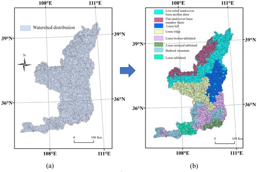
The Loess Plateau of China is the most extensive loess-covered area in the world with its unique geographical conditions, typical loess natural environment, and serious soil erosion phenomenon. As the core loess area in the Loess Plateau, Northern Shaanxi covers all the typical landform types of the Loess Plateau and has thus been the main area of loess geomorphology research (Tang et al. 2015) that attracted worldwide attention (Xiong et al. 2017). For this, it is herein selected as the study area to conduct the landform classification. Eight typical loess landform types existed in Northern Shaanxi (Tang et al. 2008) including low-relief sand-covered loess aeolian dunes (T1), flat sand-covered loess meadow basin (T2), loess hills (T3), loess ridges (T4), loess broken tablelands (T5), loess terraced tablelands (T6), bedrock mountains (T7), and loess tablelands (T8) distributed among the Northern Shaanxi (see Figure 1). These landforms with complex morphologies involve all the typical geomorphic combinations and landscape forms of the Loess Plateau (Zhou et al. 2010). Table 1 gives their morphology attributes from different aspects.

Figure 1. The Locations of the Northern Shaanxi, Loess Plateau, and eight typical landform types.

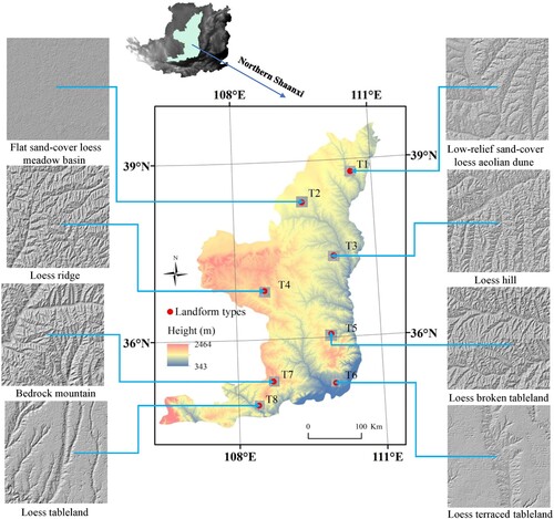
Table 1. Attributes of landform morphology in eight landforms on Loess Plateau (Xiong et al. 2018; Xiong, Tang, Strobl, & Zhu, in press).

	Mean height (m)	Mean slope density (°)	Drainage density (km/km2)	Drainage depth (m)	Terrain texture
T1	1061–1307	9.17–18.10	2.54–3.06	102–197	0.97–1.29
T2	1161–1294	0.68–2.74	0.29–0.61	13–85	1.01–1.44
T3	986–1177	20.19–24.61	2.60–3.01	133–178	2.28–2.34
T4	1415–1624	21.07–25.41	2.50–3.01	211–255	2.69–2.75
T5	843–1335	10.88–19.68	2.13–2.66	206–365	0.80–1.45
T6	417–916	0.77–7.61	0.9–1.48	60–197	0.36–0.57
T7	1309–2115	20.02–30.90	2.13–2.65	210–557	0.58–0.88
T8	926–1359	8.51–19.30	1.09–1.76	202–447	0.62–1.41

3. Materials and methodology

3.1. Materials

DEM of Loess Plateau used herein is version 2 of ASTER GDEM which was released to the public in January 2011. Version 2 of ASTER GDEM with a 30 m*30 m grid resolution is derived from an international project from NASA and METI, which has been widely accepted as a basic data source in different academic fields (Frey and Paul 2012), especially in geoscience (Florinsky, Skrypitsyna, and Luschikova 2018; Frey and Paul 2012; Xiao et al. 2018).

3.2. Methodology

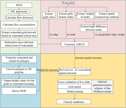
Figure 2 shows the technical route of landform classification. The proposed WOB-based landform classification scheme can be divided into four steps:(1) Dividing the whole study area with a watershed strategy (2) Establishing GWCN for each divided watershed to describe the watershed internal structure (3) Deriving WBP to quantitatively delineate watershed marginal structure (4) Training optimum landform classification model based on grid search of XGBoost (5) Classifying the watersheds and conducting landform mapping. To be specific, each step is given as follows:

Figure 2. The technique route of landform classification.

3.2.1. Watershed division at regional scale

From a geomorphological viewpoint, a geomorphologic area can be viewed as an overall system composed of massive basic watershed landform units. Watershed division can be conducted using the hydrological method based on a threshold of the watershed critical area. Before a watershed strategy division, it is crucial to determine the least critical area for the watershed unit. When the area size is too large, it may contain not only a kind of landform. On the contrary, when the area size is too small, the terrain indices may be unstable and thus can not represent the regional terrains. Scholars have found that the terrain indices on Loess Plateau tended to be stable when the watershed is greater than a threshold of 10 km² (Tang et al. 2015). It is generally adopted as the least critical area for the watershed division in previous research (Xiong et al. 2018; Cao et al. 2020; Liu et al. 2015), which is adopted herein. Then, with the flow accumulation threshold, the watershed division can be automatically conducted based on python secondary development from ArcGIS. The division process can be given into four procedures:

1. Filling depressions of DEM with Tarboton et al's method (Tarboton, Bras, and Rodriguez-Iturbe 1991).

2. Calculating flow direction (Jenson and Domingue 1988) from DEM and extracting flow accumulation (Tarboton, Bras, and Rodriguez-Iturbe 1991) from the calculated flow direction.

3. With the repeated test, determining flow accumulation threshold according to a 10 km² threshold. Extracting the watershed grid network based on flow direction and flow accumulation.

4. Dividing the area based on the stream network and flow direction distribution, which follows the least critical area of 10 km² (Strahler 1956, 1957).

3.2.2. Simulating watershed geospatial structure

3.2.2.1. Watershed geospatial structure

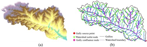
Landform spatial structure is the basic background of landform development, which is essential to landform classification (see Figure 3) (Crofts 1975; Tao, Tang, and Strobl 2012). It can be viewed as an overall composition constituted by a series of Landform components (Dehn, Gärtner, and Dikau 2001). These components constructed the basic spatial pattern of the watershed. For a watershed, the internal structure can be viewed as a hierarchical organization system consisting of gullies and gully feature nodes with close topological relationships (Zhu et al. 2018). Further, the watershed geospatial structure is a gully network formed by connecting different gully feature nodes through gullies (McDonnell et al. 2007; Zhu et al. 2012). Besides, as the most external part of the watershed, the watershed boundary is a closed boundary that surrounds the entire internal spatial structure and isolates the watershed from the outside (Marwick et al. 2018; Wang, Hao, and Xiong 2004). For this, it is generally adopted to describe the marginal structure features of the watershed. In this paper, to completely simulate the overall watershed geospatial structure, the watershed network structure and the watershed boundary are respectively adopted to construct the internal and marginal watershed spatial structure. On this basis, GWCN and WBP are used to quantitatively depict the watershed geospatial structure to further introduce the geo-attribute of the watershed.

Figure 3. Watershed and its spatial structure.

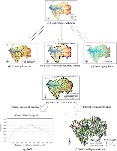
Figure 4 shows the process for deriving the watershed geospatial structure from the original morphology of the watershed. The watershed geospatial structure is simulated from two aspects: WBP which describes the marginal geospatial structure and GWCN which describes the internal geospatial structure. The detailed methods for deriving these two structures are given as follows:

Figure 4. Deriving process of watershed geospatial structure from an origin watershed.

3.2.2.2. Deriving GWCN to describe the internal spatial structure of the watershed

The deriving procedure of GWCN from an origin morphology of the watershed can be given by the following four steps:

1. Extracting gully lines. Gully lines (see Figure 4c) are derived from the stream network by hydrological analysis (Zhu et al. 2014).

2. Extracting gully feature nodes. Gully feature nodes lying on the stream network are randomly distributed in space but with the specific topology relationship of spatial connection. Strahler stream classification is adopted to classify the stream network (Strahler 1956, 1957). The watershed outlet node, gully confluence node, and gully source point (see Figure 4b) are respectively derived from a first-class, median class, and highest class of stream network.

3. Extracting spatial connectivity relation and geographic edge weight. Overlay analysis was conducted between the origin DEM and gully feature nodes to derive the height of nodes. Using the spatial query to extract the spatial connection relationship among gully feature nodes (Lin, Chen, and He 2021). Based on the spatial connection relationship, height differences of connected gully feature nodes are derived as the geographic weight of the edge.

Figure 4e shows the watershed spatial structure. Gully feature nodes are the core compositions of watershed spatial structure controlling the evolution and morphology of watershed, which possesses different characteristics (Li et al. 2020a). Watershed outlet nodes (the green nodes) represent the outermost node of the watershed. Gully confluence nodes (the red nodes), as the destination of all streams, have the largest accumulation of flow and lowest altitude. The watershed source points (the white nodes) are the origin of different streams. Red nodes are the gully confluence nodes, which are the intersect nodes between different streams. These gully feature nodes with a strong spatial topological relationship play different roles in the watershed, forming the basic skeleton of the watershed spatial structure.

We think the geospatial structure of the watershed should take into account the geographical attributes and spatial topological relations of the watershed system. For a weight complex network, weight, edges, and nodes are three fundamental factors. We first view the gully feature nodes as the nodes and view the topological connection (gully lines) as the edge. Finally, since height is the basic geo-properties of the original DEM, we view the height difference between the neighboring nodes as the geographic weight of the linked edge and constructed GWCN based on the three elements. Every edge in GWCN is endowed with a unique weight (edge weight). Further, every node is also endowed with unique geo-properties (node strength) from neighboring edge weights. With the form of the network spatial structure, GWCN describes the internal spatial compositions of the watershed and considers the geographic attribute of network composition.

3.2.2.3. Deriving WBP to describe the marginal structure of the watershed

Deriving WBP can be automatically conducted via the following four steps: (1) Converting the DEM of the watershed to derive a watershed polygon. (2) Deriving watershed boundary surface (see Figure 4d) from watershed polygon. (3) Endowing height to watershed boundary surface via 3D analysis and obtaining its 3D line. (4) Arranging and mapping WBP (see Figure 4g). The watershed boundary is the peripheral spatial structure of watersheds, which represents the basic marginal spatial structure within the watershed. Then, WBP extracted from DEM and watershed further quantitatively describes the marginal geospatial structure of the watershed.

3.2.3. Quantitatively describing the geospatial structure of the watershed

To quantitatively describe the watershed geospatial structure, we proposed diverse quantitative indices to depict the GWCN and WBP. These indices with different geo-meaning comprehensively reveal the watershed geospatial structure via describing GWCN from the aspects of node element, edge element, and whole network structure and describing WBP from surface morphology of watershed boundary and curve morphology of WBP. The corresponding algorithms, classifications, and geo-meanings for these indices were given in Tables 2 and 3 respectively.

Table 2. Quantitative indices for depicting GWCN.

Index classification	Quantitative indexes	Algorithm	Geo-meaning
Node elements and derivatives	Average node strength (NS)	$NS={\displaystyle \frac{{\sum }_{i=1}^N\left({\sum }_{j\in N_i}{a}_{ij}{w}_{ij}\right)}{N}}$ (1) $a_{ij}$ denotes the element of the network adjacency matrix; $w_{ij}$ denotes the weight of the edge that linked node$j$ and $i$; $N$ is the amount of nodes.	Revealing the surface cutting depth and landform development of certain regions Tian, Tang, and Zhao (2014).
	Network density (ND)	$d(G)=2M/[N(N-1)]$ (2) $M$ denotes the amount of edges.	Revealing the network complexity from the perspective of edge.
	Clustering coefficient (CC)	$C={\displaystyle \frac{1}{N}\sum _{i=1}^n{\displaystyle \frac{2l_i}{k_j(k_j-1)}}}$ (3) $k_j$ denotes the amount of neighboring nodes for node$i$, $l_i$ denotes the amount of edges that linked $k_i$ nodes	Revealing the compact degree of the gully feature nodes.
Edge elements and derivatives	Average path length (AL)	$AL={\displaystyle \frac{1}{{\displaystyle \frac{1}{2}N(N-1)}}\sum _{i>j}{d}_{ij}}$ (4) $d_{ij}$ the length between node $j$ and $i$.	Revealing the connectivity among gully feature nodes.
	Gully line density (GL)	$GL={\displaystyle \frac{G}{S}}$ (5) $G$ denotes the sum of the length for all the gully lines, $A$ denotes the area size of the watershed.	Describing the degree of geomorphic fragmentation and geomorphic complexity.
	Network diameter (ND)	$ND=\sum _{i,j}\max (d_{ij})$ (6) $\max (d_{ij})$is the function to obtain the max values of the dataset $d_{ij}$.	Reflecting the development degree of the main gully.
Network structure and derivatives	Structure entropy (SE)	$H_i={\displaystyle \frac{S_i}{{\sum }_{i=1}^n{S}_i}}$ (7) $SE=-\sum _{i=1}^n{H}_i\ln H_i$ (8) $H_i$ denotes the importance of node $i$; $S(i)$ denotes the node strength of the node $i$.	Reflecting the stability of a gully network in one region and thus measures the gully evolution.
	Fractal dimension (FD)	There are many different methods for calculating FD based on different functions. This paper adopted the box dimension to quantize the watershed structure (Tricot 1994).	Reflecting the degree of fragmentation and self-similarity of landforms.
	Modularity (M)	$MM={\displaystyle \frac{1}{2M}\sum _{i,j}(w_{ij}-k_i{k}_j/(2M)\gamma (l_i,l_j)}$ (9) $k_i$ denotes the node strength for node $i$; $\gamma (C_i,C_j)$ denotes the function which defines $\gamma$ as 1 if $l_i=l_j$ and defines $\gamma$ as 0 in other cases;$l_i$ denotes the community to that node $i$ belonged.	Revealing the watershed agglomeration effect.

Table 3. Quantitative indices for depicting WBP.

Index classification	Quantitative Indexes	Algorithm	Geo-meaning
Surface morphology and derivatives	Mean height ($\overline{H}$)	$\overline{H}={\displaystyle \frac{1}{N}\sum _{i=1}^N{H}_i}$ (10) $N$ is the number of grids in the watershed boundary.	Revealing the average elevation of the watershed boundary topography.
	Height standard deviation $(\sigma )$	$\sigma =\sqrt{{\displaystyle \frac{{\sum }_{i=1}^N(H_i-\overline{H})}{N-1}}}$ (11)	Reflecting the discrete degree of the height in the watershed boundary.
	Roughness (R)	$R=R_s/R_O$ (12) Rs denotes the surface length of the watershed boundary; $R_O$ denotes the projected length of the watershed Boundary.	Describing the slope degree of the watershed boundary.
	Watershed boundary density (D)	$D=R_s/A$ (13) A denotes watershed area.	Describing the slope degree of the watershed boundary.
Curve morphology and derivatives	Fluctuating frequency (F)	$\mathrm{F}={\displaystyle \frac{F_r+F_s}{N}}$ (14) $F_r+F_s$ are the number of wave crest and wave trough respectively.	Describing the intensity of fluctuation in the WBP and somewhat revealing the landform evolution of the watershed.
	Skewness ($\mathrm{S}$)	$\mathrm{S}=\sqrt{{\displaystyle \frac{1}{6n}}}\sum _{i=1}^n{\left({\displaystyle \frac{N_i-\overline{H}}{\sigma }}\right)}^3$ (15) $\sigma$ is the standard deviation of the sample dataset in the watershed boundary profile.	Reflecting the unsymmetry of the WBP distribution.
	Kurtosis (K)	$\mathrm{K}={\displaystyle \frac{\mathrm{E}[{(N_i-\overline{H})}^4]}{{(E[{(N_i-\overline{H})}^2])}^2}}$ (16) $\mathrm{E}$ represents the function used to obtain the mean value of the variables in the parentheses.	Reflecting the flatness of the WBP distribution.

3.2.4. XGBoost

XGBoost is a cutting-edge ensemble learning model based on the Gradient Boosting Decision Tree (GBDT) with less training time and high accuracy (Chen and Guestrin 2016; Ke et al. 2019). XGBoost utilized the summation of the predicted values of the samples in each tree to realize the prediction. A key improvement of XGBoost from GBDT is that it introduces regular terms to the objective function, which effectively constrains the growth structure of the tree and simultaneously avoids overfitting problems (Ma et al. 2018). In addition, XGBoost conducted the second-order approximation to the loss function, which speeds up the descent of the loss function and thus accelerates the model iteration. It is widely employed in different academic fields and shows well performance (Lösing and Ebbing 2021; Ogunleye and Wang 2020; Zhang et al. 2018; Zheng, Yuan, and Chen 2017). Many machine learning methods such as random forest (RF), and support vector machine (SVM) have been extensively used in landform classification. However, as a new GBDT method, the applications of XGBoost in landform classification are few. A series of studies proved that, in many cases, XGBoost showed better performance than the above-mentioned machine learning methods (Cao et al. 2021; Moorthy et al. 2020; Yan et al. 2020). We herein adopted it to conduct landform classification of the loess landforms.

3.2.5. Experimental setup and evaluation criterion

With 30 samples for each landform type, 240 watersheds in Northern Shaanxi were selected by expert experiences as the training dataset. Nine indices were extracted as the input feature variables to quantitatively describe the geospatial structure from the viewpoints of node element, edge element, and overall structure. These feature variables are normalized within the boundary (0–1) to avoid dimension differences (Lu et al. 2021).

We adopted grid search to search for the optimum parameter composition of the XGBoost model (Wang et al. 2020). Different evaluation scores of the parameter compositions can be given by conducting the cross-validation of five folds to the training dataset. By comparing the scores of different parameter compositions, we can estimate the performance of these parameter compositions and thus select the optimum parameter composition. In this paper, after the grid search, we determine the learning rate as 0.21, the maximum depth as 3, the number of iterations as 375, and the number of trees as 50.

4. Results

4.1. Landform classification in Northern Shaanxi

Based on the minimum watershed area size of 10 km², we firstly conducted the watershed division of the study area via a series of hydrological methods (see Figure 5a). The whole sample area has been divided into 4612 Watersheds. Each watershed unit possesses specific terrain features and geospatial structure. All the watershed units are simulated via the proposed method to construct the geospatial structures of watersheds and quantitatively described by the proposed index system. On this basis, we construct the optimum landform classification model of XGBoost in terms of watershed geospatial structure. Finally, we conducted landform classification on the study area. Figure 5b presents the classified landforms of northern Shaanxi.

Figure 5. Landform classification process.

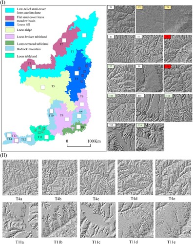
To clearly present the overall landform distribution, the delineated inter-watersheds were merged into their neighboring watersheds (Sun and Tang 2013; Xiong et al. 2018). Figure 6 presents the classified fourteen regions in terms of the eight key landform types. For the different regions which attribute to the same landform types, the rectangular windows are derived from similar texture features and surface morphologies. For the regions of different landforms, the rectangular windows are derived from similar texture features and surface morphologies. Besides, The topography within the same regions shows the topographic homogeneity. Specifically, we discussed the regional-scale landform classification result from two aspects as follows.

Figure 6. Landform division via merging the neighboring watersheds. In (I), to fully present the surface morphology of the divided regions, fourteen rectangular analysis windows from regions of T11 to T14 were randomly derived to detail show the intermediate classification results. Besides, In (II), six rectangular analysis windows are derived from the regions T4 and other windows are derived from T11, which presents the surface morphology of the terrains in the same region.

Clear regional boundaries and spatial aggregation. Obvious boundaries are exhibited between different landforms. The landforms within a specific region show topographical homogeneity and obvious spatial aggregation. The aggregation effect of loess landforms embodies the First Law of Geography. Noted that a boundary line demarcates the scope of desert area (T1) in the northwest area. T1 is a region of Mu Us Desert, which is quite different from the main loess landforms on the Loess Plateau in terms of terrain features and geomorphic mechanisms. Delineating the boundary line between the Mu Us Desert and other loess areas is of great guiding significance to the monitoring and management of the Mu Us Desert. Loess hill (T4), loess ridge (T5), and three kinds of loess tableland landforms (T6, T8, T9, T11) are three special loess landform regions in Loess Plateau that are widely known in the world. The differences between them reflect the formation process and erosion situation of surface morphology for different loess landforms. These three landforms are located in the area that has been rising intermittently since the Quaternary and is close to the Yellow River, which is greatly influenced by the decline of the Yellow River base level. Since they are the most prone areas to soil erosion, determining the coverage range and their boundary line is of great significance to study and control soil and water loss.

Gradual transitional variation in space. There is a transitional relationship between landform distribution, which corresponds to the characteristics of the gradual evolution of the landform type in space (Stevens et al. 2013; Zhao and Cheng 2014). E.g. T1 is the transition zone between arid aeolian geomorphology and loess hilly-gully geomorphology, which is a region with low loess hills and is affected by wind and sand. Besides, a spatial transitional variation of Low-relief sand-cover loess aeolian dune (T1), loess hill (T4), loess ridge (T5), loess broken tableland (T6 or T9), loess tableland (T11), from northwest to the southeast was consistent with the evolution process by field surveys and previous studies (Tang et al. 2008, 2015; Zhu et al. 2014). These landforms are intersected results formed by the loess erosion from the Yellow River and the loess deposition from the northwestern desert areas (Xiong et al. 2014). These spatial variations with transitional relationships increase our understanding of the evolution process and internal mechanism of landforms in the Loess Plateau and reveal the transitional process of different landforms.

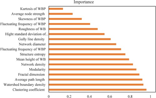
Feature importances (i.e. the contribution of different features) can be measured via the XGBoost (Shi et al. 2019). Figure 7 presents the importance of the features from the watershed geospatial structure. Clearly, features from GWCN and WBP have both great contributions to the landform classification process. But some features from GWCN seemed to contribute much more than that of WBP. It might suggest that the indices describing internal spatial structure have better responses to recognize landforms than that describing marginal spatial structure.

Figure 7. Feature importances of different indices.

4.2. Evaluating classification performance of the proposed method

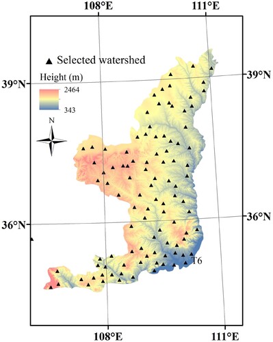
In this study, 100 watersheds randomly located in Northern Shaanxi were selected to evaluate the landform classification result (see Figure 8). To ensure the fairness and comprehension of the verifying result, the selected watersheds covered all landform types and were distributed among the Northern Shaanxi as much as possible.

Figure 8. Locations of the selected watersheds.

The landform labels of these watersheds are referred to the Geomorphological Atlas of the People's Republic of China (1:1,000,000), which is a key landform reference system of the Geomorphological division of China (Li et al. 2020b). Besides, to ensure the precision of the landform labels of these watersheds, we also conducted an artificial examination in these watersheds by experts. The landform types of selected watersheds, following the general process of visual interpretation of geomorphology, were determined by visual interpretation from the expert experience via topographic maps and aerial photographs (Argialas 1995; Du et al. 2019; Mokarram and Sathyamoorthy 2018). Table 4 shows the function of different datasets that were used to verify these landform labels. The aerial photographs are the remote sensing images which are 1 m high-resolution images provided by Google Earth. The shaded relief map has great visual features including landform texture and shape features, showing more geomorphological significance than remote sensing images. Finally, the topographic map is generally adopted to reveal the landform structure (Du et al. 2019). Figure 9 shows the process of determining the landform types of selected watersheds.

Figure 9. The process to determine the landform types of selected watersheds.

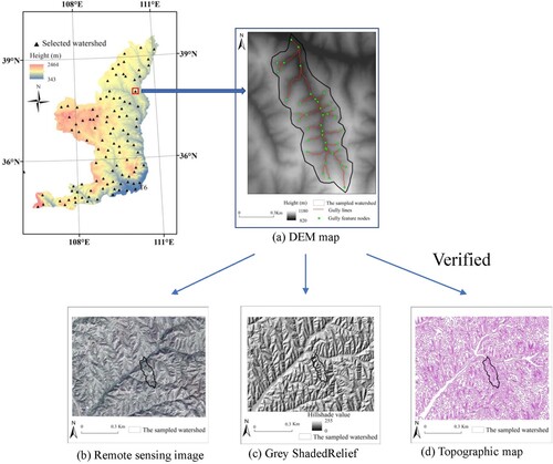
Table 4. Information and function of the used datasets in the accuracy assessment.

Data type	Resolution	Function
Geomorphological Atlas of the People’s Republic of China	Vector	Determing the landform labels
DEM	30 m	Reflecting terrain relief and height.
Aerial photograph	1m	Revealing landform morphology
Topographic map	30 m	Reflecting landform structure
Shaded relief map	30 m	Providing visual features about texture and shape feature

Table 5 presents the confusion matrix of classification results for selected watersheds. The proposed method showed remarkable performance with an accuracy higher than 80% for each landform, indicating its great universality in different landform types. Overall accuracy reached 89% with a Kappa coefficient of 0.87, which suggested its well comprehensive performance. Besides, compared with the classification result in previous research on Northern Shaanxi, the developed method has a 2.7–6.6% accuracy improvement (Tang et al. 2008; Xiong et al. 2021; Cao et al. 2020).

Table 5. Confusion matrix from classification results based on the developed method.

	Classification via the proposed method
Actual landforms		T1	T2	T3	T4	T5	T6	T7	T8	Accuracy (%)
	T1	13	1	0	0	0	1	1	1	81.25
	T2	0	12	1	0	0	0	0	0	92.3
	T3	0	0	12	1	0	0	0	0	92.3
	T4	0	0	1	14	1	0	0	0	87.5
	T5	1	0	0	0	10	1	0	1	83.3
	T6	0	0	0	0	0	8	0	0	100
	T7	0	0	0	0	0	0	11	1	91.7
	T8	0	0	0	0	0	0	1	9	90.0
	Overall accuracy: 89%
	Kappa coefficient: 0.87

5. Discussion

5.1. Influence of the training datasets on the landform classification

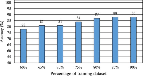
To study the influence of the number of training datasets on the landform classification in our method, we conducted other six experiments. To be specific, 60%,65%,70%,75%, 80%, and 85% of the origin training data sets were used as new training data sets to construct the landform classification model. Based on these models, we conducted the landform classification in the selected 100 watersheds and compare their accuracies (see Figure 10). With the increase of training data sets, the recognition accuracy of the proposed method shows a steady upward trend. Even only using 60% of the training dataset, the overall accuracy reached 78%, which suggested the effectiveness of the proposed method. The average increase in accuracy is about 2%. When the training dataset increase to 90%, the accuracy does not increase further. With the increase of training data sets, the recognition accuracy of the proposed method shows a steady upward trend. The average increase in accuracy is about 2%. These results convincingly prove that the proposed method has good robustness.

Figure 10. The variation of the accuracy with the increase of training dataset.

5.2. Comparison with methods based on fusion datasets of landform morphologies

5.2.1. Differences and similarities in the proposed method with previous studies

Previous studies conducted landform classification on Northern Shaanxi via a series of terrain indices (Tang et al. 2008; Xiong et al. 2018). The similarities and differences between the landform division of Northern Shaanxi via previous scholars and that in this paper can be discussed in four aspects as follows.

1. Division scale. Tang et al utilized 81 experimental regions to simulate the spatial distribution of landform features. Xiong et al and this study considered all the watershed units.

2. Characterization method of landforms. Xiong et al used a series of terrain indices and texture indices to quantify the landform features from different aspects. Tang et al quantify the landform features from the slope of surface morphology. This paper utilized watershed geospatial structure to characterize the landform features.

3. Landform classification strategy. Xiong et al and the present study performed landform classification via a watershed-based strategy, while Tang et al classified landforms based on a pix-based strategy.

4. Landform classification frame. Tang et al used Iterative Self-Organizing Data Analysis Technique to perform the unsupervised classification. Xiong et al used prior knowledge and the decision tree method to conduct the unsupervised classification. This study utilized the XGBoost and expert experiences to conduct supervised classification.

5.2.2. Compare the performance of the proposed method with that of the previous method

Previous studies on landform classification generally adopted terrain indices or texture indices to classify landforms (Lin, Chen, and He 2021; Mokarram and Sathyamoorthy 2018). Fusion of terrain indices and texture indices is a key methodology in landform classification, which showed better accuracy than single-class features (Du et al. 2019; Zhao et al. 2017). Scholars suggested that eighteen indices which are composed of topographic indices and texture indices are the most important in the study of landform classification in northern Shaanxi (Cao et al. 2020). To fairly and concretely compare the classification performance of the developed method with previous methods, we used the eighteen indices to conduct landform classification based on the selected watersheds.

To be precise, fusion datasets included fourteen derivatives reflecting the terrain features (the standard deviation of terrain relief, elevation standard deviation, mean cutting depth, slope standard deviation, the standard deviation of cutting depth, average plane curvature, mean slope, the standard deviation of plane curvature, mean terrain relief, mean elevation, the standard deviation of profile curvature, mean aspect, the standard deviation of aspect, and mean profile curvature) and four derivatives reflecting the texture features (texture contrast, texture angular second moment, texture information entropy, and texture inverse difference moment) were derived from the training dataset of watersheds. For this, the corresponding optimal classification model based on XGBoost was also established via a grid search with five-fold cross-validation.

Table 6 presents the confusion matrix of classification results for the selected watersheds. By contrast, for different landform types, it is clear that the proposed method performs well in landform classification with comparative or better accuracy in the landform classification than previous methods using the fusion of terrain indices and texture indices (see Figure 11). The overall accuracy of the fusion dataset was 84% and the kappa coefficient is 82.7%, which was worse than that of the proposed method.

Figure 11. The accuracy comparison in terms of eight landform types from two methods.

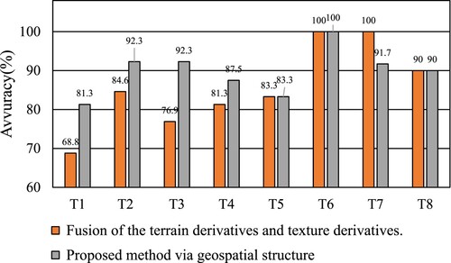
Table 6. Confusion matrix from classification results based on the fusion datasets.

	Classification via fusion of terrain indices and texture indices
Actual landforms		T1	T2	T3	T4	T5	T6	T7	T8	Accuracy (%)
	T1	11	3	0	0	0	0	1	1	68.8
	T2	2	11	0	0	0	0	0	0	84.6
	T3	0	0	10	2	1	0	0	0	76.9
	T4	0	0	2	13	1	0	0	0	81.3
	T5	1	0	0	1	10	1	0	0	83.3
	T6	0	0	0	0	0	8	0	0	100.0
	T7	0	0	0	0	0	0	12	0	100.0
	T8	0	0	0	0	0	0	1	9	90.0
	Overall accuracy: 84%
	Kappa coefficient: 0.83

Besides, it is noted that two landform combinations that were easily confused in previous research showed better accuracy based on the watershed geospatial structure. It may suggest the proposed method tends to perform better in recognizing the landform types with obvious geomorphologic spatial structure. To be specific, T1 (Flat sand-cover loess meadow basin) and T2 (Low-relief sand-cover loess aeolian dune) are easily confused since their flat and wide geographic surface with low terrain relief, which lacks terrain and morphology features (Cao et al. 2020). In the method based on the fusion dataset, the accuracies only achieved 68.8% and 84.6%, whilst accuracies reached 81.3% and 92.3% in the method based on watershed geospatial structure.

Alternatively, the distinguishment between the loess landforms especially for T4 (loess hill) and T5 (loess ridge) is generally challenging in previous studies (Xiong et al. 2014; Liu et al. 2015). Simultaneously, because of their similar shapes and vague definitions, it is also difficult to distinguish them by experts’ prior knowledge (Li et al. 2020b), which forms a potential gap in the current landform classification. In this case, the accuracies achieved 76.9% and 81.3% in the method based on the fusion dataset, whereas accuracies reached 92.3% and 87.5% in the method based on watershed geospatial structure. Thus, the proposed method may be a better solution to classify some similar or complex landform combinations, therefore fairly emphasizing the significance of this study.

To conclude, experiment results suggest that the proposed method is an effective method in landform classification, which seemed to show excellent performance in some landforms where the terrain feature or morphology is not obvious or complex. The landform classification using watershed geospatial structure seemed to produce better results in classifying the loess landforms. Loess Plateau is the typical gully area in the world, which has a diverse spatial structure of gully landforms. Thus, it may produce a positive response to the geospatial structure of the watershed on the Loess Plateau that outperformed the previous methods.

5.3. Innovations and limitations of the present study

This work developed the complex network theory on landform classification and mapping. To our knowledge, it may be the first application of complex network theory on landform classification. The current research on the complex network in earth science is generally the theoretical analysis of various scientific problems with little practical application to our knowledge. Our work is a successful attempt at complex network theory from theoretical analysis to practical application.

On the methodological side, this work innovatively provided a landform classification method based on the watershed geospatial structure. The spatial structure of landforms is a key aspect in quantitatively describing landforms from the macro scale. Within the watershed spatial structure, the spatial relationship and spatio-temporal variation of terrain feature nodes can reflect the basic situation of geomorphic development and evolution. However, there is no corresponding study of landform classification using landform spatial structure, which brings a potential gap in this field. The current research so far on landform classification is generally for the terrain feature or texture feature that is from morphology. Using terrain indices or texture indices by neighborhood analysis reveals local landform attributes, which failed to reveal terrain structure characteristics at a macro scale. The present study proposed a method to effectively construct the watershed spatial structure. Besides, it introduced geo-attributes to the watershed spatial structure using the weighted complex network theory and WBP model. It provides features by excavating the watershed geospatial structure, which differs from the conventional approach based on terrain morphology and therefore fills the potential gap in the field.

On the other hand, noted that WOB landform classification is the new highlight in the field of landform classification. On the application side, the proposed method is a kind of method that is specifically developed for WOB landform classification. Besides, it provided fresh viewpoints and thus further develop this classification frame of watershed-based strategy.

The developed method seemed to possess better accuracy and universality than the previous research that is based on texture indices or terrain indices. It may have significant accuracy in classifying landforms with low morphological or terrain differentiation. T4 and T5 have broken terrain surfaces and complex landform morphologies, whilst T1 and T2 have low terrain relief with unobvious morphological characteristics. The classification of two landform combinations is generally difficult and complex, which has brought limitations to the current landform classification field and knowledge bottlenecks for some scholars and terrain experts (Xiong et al. 2018; Zhao et al. 2017; Cao et al. 2020; Liu et al. 2015). However, what is striking is that the proposed method from the angle of the watershed geospatial structure seems to effectively relieve the confusion of these landforms and significantly enhance recognition accuracy.

However, some limitations exist in the present study, which is given as follows:

1. The quantification of watershed spatial structure is inevitably affected by DEM resolution and thus affects the accuracy of landform classification. However, it is an unavoidable problem for digital terrain analysis based on DEM.

2. Some landform components, such as the gully shoulder line, might be also used for landform classifications. However, this paper mainly classifies landforms from the perspective of the internal and external marginal two-layer structure of landforms.

6. Conclusions

In this study, we utilized GWCN and WBP to quantitatively delineate the complete geospatial structure of watersheds and consequently developed a novel WOB landform classification method for automatically classifying the loess landforms. we draw the following conclusions:

1. Landform distribution has clear spatial aggregation and gradual transition variation. Different geomorphic regions with significant topographic homogeneity reveal the internal conditions of loess deposition and runoff erosion in different regions. Gradual variation with transitional relationship showed the loess landform evolution under the unique loess environment.

2. Landform distribution has clear regional boundaries. The different boundaries are formed by comprehensive results under Yellow River erosion, loess deposition, and tectonic differentiation.

3. The proposed method in landform classification showed full availability and robustness. The classification results achieved an accuracy of 89% and a kappa coefficient of 0.87, which sufficiently demonstrated its effectiveness and remarkable performance.

4. The proposed method produced better classification results in distinguishing some similar and complex landforms.

In brief, this study provided a new and effective method for WOB landform classification utilizing the watershed geospatial structure. It is based on the perspective of landform spatial structure at the macro scale, which is different from previous studies based on landform morphology at the regional scale and seemed to show better performance.

Disclosure statement

No potential conflict of interest was reported by the authors.

Correction Statement

This article has been corrected with minor changes. These changes do not impact the academic content of the article.

Additional information

Funding

This work was supported by the National Natural Science Foundation of China [grant numbers 41771423, 41491339, 41771423, 41491339, 41930102, and 41601408, 41771423, 41930102, 41601408, and 41491339].

References

- Abe, S., and N. Suzuki. 2006. “Complex-Network Description of Seismicity.” Nonlinear Processes in Geophysics 13 (2): 145–150.
- Argialas, D. 1995. “Towards Structured-Knowledge Models for Landform Representation.” Zeitschrift für Geomorphologie 101: 85–108.
- Blaschke, T. 2010. “Object Based Image Analysis for Remote Sensing.” ISPRS Journal of Photogrammetry and Remote Sensing 65 (1): 2–16.
- Blaschke, T., G. J. Hay, M. Kelly, S. Lang, P. Hofmann, E. Addink, R. Q. Feitosa, F. Van der Meer, H. Van der Werff, and F. Van Coillie. 2014. “Geographic Object-Based Image Analysis–Towards a New Paradigm.” ISPRS Journal of Photogrammetry and Remote Sensing 87: 180–191.
- Cao, Z., Z. Fang, J. Yao, and L. Xiong. 2020. “Loess Landform Classification Based on Random Forest.” Journal of Geo-information Science 22 (3): 452–463.
- Cao, D., Y. Ma, L. Sun, and L. Gao. 2021. “Fast Observation Simulation Method Based on XGBoost for Visible Bands Over the Ocean Surface Under Clear-sky Conditions.” Remote Sensing Letters 12 (7): 674–683.
- Cao, M., G. Tang, F. Zhang, and J. Yang. 2013. “A Cellular Automata Model for Simulating the Evolution of Positive–Negative Terrains in a Small Loess Watershed.” International Journal of Geographical Information Science 27 (7): 1349–1363.
- Caratti, J. F., J. A. Nesser, and C. Maynard. 2004. “Watershed Classification Using Canonical Correspondence Analysis and Clustering Techniques: A Cautionary Note.” Journal of the American Water Resources Association 40 (5): 1257–1268.
- Chen, T., and C. Guestrin. 2016. “Xgboost: A Scalable Tree Boosting System.” Proceedings of the 22nd ACM Sigkdd International Conference on Knowledge Discovery and Data, 785–794.
- Chen, J., F. Li, Y. Pu, G. Tang, C. Wang, and T. Zhang. 2007. “Quantitative Analysis and Spatial Distribution of Slope Spectrum: A Case Study in the Loess Plateau in North Shaanxi Province, Geoinformatics 2007: Geospatial Information Science.”
- Condon, L. E., K. H. Markovich, C. A. Kelleher, J. J. McDonnell, G. Ferguson, and J. C. McIntosh. 2020. “Where is the Bottom of a Watershed?” Water Resources Research 56 (3): e2019WR026010.
- Crofts, R. S. 1975. “The Landscape Component Approach to Landscape Evaluation.” Transactions of the Institute of British Geographers 66: 124–129.
- Dehn, M., H. Gärtner, and R. Dikau. 2001. “Principles of Semantic Modeling of Landform Structures.” Computers & Geosciences 27 (8): 1005–1010.
- Donges, J. F., Y. Zou, N. Marwan, and J. Kurths. 2009. “Complex Networks in Climate Dynamics.” The European Physical Journal Special Topics 174 (1): 157–179.
- Drăguţ, L., and C. Eisank. 2011. “Object Representations at Multiple Scales From Digital Elevation Models.” Geomorphology 129 (3-4): 183–189.
- Drăguţ, L., and C. Eisank. 2012. “Automated Object-Based Classification of Topography From SRTM Data.” Geomorphology 141-142: 21–33.
- Du, L., X. You, K. Li, L. Meng, G. Cheng, L. Xiong, and G. Wang. 2019. “Multi-modal Deep Learning for Landform Recognition.” ISPRS Journal of Photogrammetry and Remote Sensing 158: 63–75.
- Evans, I. S. 2012. “Geomorphometry and Landform Mapping: What is a Landform?” Geomorphology 137 (1): 94–106.
- Ferguson, R. I. 2003. “Emergence of Abrupt Gravel to Sand Transitions Along Rivers Through Sorting Processes.” Geology 31 (2): 159–162.
- Florinsky, I., T. Skrypitsyna, and O. Luschikova. 2018. “Comparative Accuracy of the AW3D30 DSM, ASTER GDEM, and SRTM1 DEM: A Case Study on the Zaoksky Testing Ground, Central European Russia.” Remote Sensing Letters 9 (7): 706–714.
- Frey, H., and F. Paul. 2012. “On the Suitability of the SRTM DEM and ASTER GDEM for the Compilation of Topographic Parameters in Glacier Inventories.” International Journal of Applied Earth Observation and Geoinformation 18: 480–490.
- Fu, B., Y. Liu, Y. Lü, C. He, Y. Zeng, and B. Wu. 2011. “Assessing the Soil Erosion Control Service of Ecosystems Change in the Loess Plateau of China.” Ecological Complexity 8 (4): 284–293.
- Gan, C., X. Yang, W. Liu, Q. Zhu, J. Jin, and L. He. 2014. “Propagation of Computer Virus Both Across the Internet and External Computers: A Complex-Network Approach.” Communications in Nonlinear Science and Numerical Simulation 19 (8): 2785–2792.
- Halverson, M. J., and S. W. Fleming. 2015. “Complex Network Theory, Streamflow, and Hydrometric Monitoring System Design.” Hydrology and Earth System Sciences 19 (7): 3301–3318.
- Hammond, E. H. 1964. “Analysis of Properties in Land Form Geography: an Application to Broad-Scale Land Form Mapping.” Annals of the Association of American Geographers 54 (1): 11–19.
- Hay, G., and G. Castilla. 2006. “Object-Based Image Analysis: Strengths, Weaknesses, Opportunities and Threats (SWOT).” Proc. 1st Int. Conf. OBIA, 4–5.
- Hiller, J., and M. Smith. 2008. “Residual Relief Separation: Digital Elevation Model Enhancement for Geomorphological Mapping.” Earth Surface Processes and Landforms 33 (14): 2266–2276.
- Hofmann, S. G., J. Curtiss, and R. J. McNally. 2016. “A Complex Network Perspective on Clinical Science.” Perspectives on Psychological Science 11 (5): 597–605.
- Huang, S., and J. Ferng. 1990. “Applied Land Classification for Surface Water Quality Management: II. Land Process Classification.” Journal of Environmental Management 31 (2): 127–141.
- Jasiewicz, J., and T. F. Stepinski. 2013. “Geomorphons—a Pattern Recognition Approach to Classification and Mapping of Landforms.” Geomorphology 182: 147–156.
- Jenson, S. K., and J. O. Domingue. 1988. “Extracting Topographic Structure From Digital Elevation Data for Geographic Information System Analysis.” Photogrammetric Engineering and Remote Sensing 54 (11): 1593–1600.
- Kaluza, P., A. Kölzsch, M. T. Gastner, and B. Blasius. 2010. “The Complex Network of Global Cargo Ship Movements.” Journal of the Royal Society Interface 7 (48): 1093–1103.
- Ke, G., Z. Xu, J. Zhang, J. Bian, and T. Y. Liu. 2019. “DeepGBM: A Deep Learning Framework Distilled by GBDT for Online Prediction Tasks.” In Proceedings of the 25th ACM SIGKDD International Conference on Knowledge Discovery & Data Mining, 384–394.
- Kilic Gul, F. 2018. “Geomorphometry-Automatic Landform Classification.” Journal of Geography-Cografya Dergisi 36: 15–26.
- Kramm, T., D. Hoffmeister, C. Curdt, S. Maleki, F. Khormali, and M. Kehl. 2017. “Accuracy Assessment of Landform Classification Approaches on Different Spatial Scales for the Iranian Loess Plateau.” ISPRS International Journal of Geo-Information 6 (11): 366.
- Lee, S., S. Hwang, S. Lee, H. Hwang, and H. Sung. 2009. “Landscape Ecological Approach to the Relationships of Land Use Patterns in Watersheds to Water Quality Characteristics.” Landscape and Urban Planning 92 (2): 80–89.
- Li, X., and Z. Dong. 2011. “Detection and Prediction of the Onset of Human Ventricular Fibrillation: An Approach Based on Complex Network Theory.” Physical Review E 84 (6): 062901.
- Li, C., F. Li, Z. Dai, X. Yang, X. Cui, and L. Luo. 2020a. “Spatial Variation of Gully Development in the Loess Plateau of China Based on the Morphological Perspective.” Earth Science Informatics 13 (4): 1103–1117.
- Li, S., L. Xiong, G. Tang, and J. Strobl. 2020b. “Deep Learning-Based Approach for Landform Classification From Integrated Data Sources of Digital Elevation Model and Imagery.” Geomorphology 354: 107045.
- Li, M., X. Yang, J. Na, K. Liu, Y. Jia, and L. Xiong. 2017. “Regional Topographic Classification in the North Shaanxi Loess Plateau Based on Catchment Boundary Profiles.” Progress in Physical Geography: Earth and Environment 41 (3): 302–324.
- Lin, S., N. Chen, and Z. He. 2021. “Automatic Landform Recognition From the Perspective of Watershed Spatial Structure Based on Digital Elevation Models.” Remote Sensing 13 (19): 3926.
- Liu, S., F. Li, R. Jiang, R. Chang, and W. Liu. 2015. “Automatic Slope Spectrum Identification of Loess Geomorphic Types.” Journal of Geo-information Science 17 (10): 1234–1242. (in Chinse).
- Lösing, M., and J. Ebbing. 2021. “Predicting Geothermal Heat Flow in Antarctica With a Machine Learning Approach.” Journal of Geophysical Research: Solid Earth 126 (6): e2020JB021499.
- Lu, M., Q. Zhao, J. Zhang, K. M. Pohl, L. Fei-Fei, J. C. Niebles, and E. Adeli. 2021. “Metadata Normalization.” In Proceedings of the IEEE/CVF Conference on Computer Vision and Pattern Recognition, 10917–10927.
- Ma, X., J. Sha, D. Wang, Y. Yu, Q. Yang, and X. Niu. 2018. “Study on A Prediction of P2P Network Loan Default Based on the Machine Learning LightGBM and XGboost Algorithms According to Different High Dimensional Data Cleaning.” Electronic Commerce Research and Applications 31: 24–39.
- MacMillan, R., R. K. Jones, and D. H. McNabb. 2004. “Defining a Hierarchy of Spatial Entities for Environmental Analysis and Modeling Using Digital Elevation Models (DEMs).” Computers, Environment and Urban Systems 28 (3): 175–200.
- Marwick, B., P. Hiscock, M. Sullivan, and P. Hughes. 2018. “Landform Boundary Effects on Holocene Forager Landscape Use in Arid South Australia.” Journal of Archaeological Science: Reports 19: 864–874.
- McDonnell, J., M. Sivapalan, K. Vaché, S. Dunn, G. Grant, R. Haggerty, C. Hinz, R. Hooper, J. Kirchner, and M. Roderick. 2007. “Moving Beyond Heterogeneity and Process Complexity: A New Vision for Watershed Hydrology.” Water Resources Research 43 (7).
- Mokarram, M., and D. Sathyamoorthy. 2018. “A Review of Landform Classification Methods.” Spatial Information Research 26 (6): 647–660.
- Monteiro, F. C., and A. Campilho. 2008. “Watershed Framework to Region-Based Image Segmentation.” 2008 19th International Conference on Pattern Recognition, IEEE, 1–4.
- Moorthy, S. M. K., K. Calders, M. B. Vicari, and H. Verbeeck. 2020. “Improved Supervised Learning-Based Approach for Leaf and Wood Classification From LiDAR Point Clouds of Forests.” IEEE Transactions on Geoscience and Remote Sensing 58 (5): 3057–3070.
- Moreno, M., S. Levachkine, M. Torres, and R. Quintero. 2004. “Landform Classification in Raster Geo-Images.” In Progress in Pattern Recognition, Image Analysis and Applications, edited by A. Sanfeliu, J. F. M. Trinidad, and J. A. C. Ochoa, 558–565. Berlin, Heidelberg: Springer
- Na, J., H. Ding, W. Zhao, K. Liu, G. Tang, and N. Pfeifer. 2021. “Object-Based Large-Scale Terrain Classification Combined with Segmentation Optimization and Terrain Features: A Case Study in China.” Transactions in GIS 25 (6): 2939–2962.
- Ogunleye, A., and Q. Wang. 2020. “XGBoost Model for Chronic Kidney Disease Diagnosis.” IEEE/ACM Transactions on Computational Biology and Bioinformatics 17 (6): 2131–2140.
- O'Neill, R. V., C. T. Hunsaker, K. B. Jones, K. H. Riitters, J. D. Wickham, P. M. Schwartz, I. A. Goodman, B. L. Jackson, and W. S. Baillargeon. 1997. “Monitoring Environmental Quality at the Landscape Scale: Using Landscape Indicators to Assess Biotic Diversity, Watershed Integrity, and Landscape Stability.” BioScience 47 (8): 513–519.
- Prima, O. D. A., A. Echigo, R. Yokoyama, and T. Yoshida. 2006. “Supervised Landform Classification of Northeast Honshu From DEM-Derived Thematic Maps.” Geomorphology 78 (3-4): 373–386.
- Rong, J., and Y. L. Pan. 2012. “Accuracy Improvement of Graph-Cut Image Segmentation by Using Watershed.” Advanced Materials Research 341–342: 546–549.
- Saadat, H., R. Bonnell, F. Sharifi, G. Mehuys, M. Namdar, and S. Ale-Ebrahim. 2008. “Landform Classification From a Digital Elevation Model and Satellite Imagery.” Geomorphology 100 (3-4): 453–464.
- Saha, K., N. A. Wells, and M. Munro-Stasiuk. 2011. “An Object-Oriented Approach to Automated Landform Mapping: A Case Study of Drumlins.” Computers & Geosciences 37 (9): 1324–1336.
- Schillaci, C., and A. Braun. 2015. “Terrain Analysis and Landform Recognition.” Geomorphological Techniques.
- Shi, X., Y. Wong, M. Z.-F. Li, C. Palanisamy, and C. Chai. 2019. “A Feature Learning Approach Based on XGBoost for Driving Assessment and Risk Prediction.” Accident Analysis & Prevention 129: 170–179.
- Singh, R., K. K. Garg, S. P. Wani, R. Tewari, and S. Dhyani. 2014. “Impact of Water Management Interventions on Hydrology and Ecosystem Services in Garhkundar-Dabar Watershed of Bundelkhand Region, Central India.” Journal of Hydrology 509: 132–149.
- Sivakumar, B., C. E. Puente, and M. L. Maskey. 2018. “Complex Networks and Hydrologic Applications.” In Advances in Nonlinear Geosciences, 565–586. Cham: Springer.
- Stevens, T., A. Carter, T. Watson, P. Vermeesch, S. Andò, A. Bird, H. Lu, E. Garzanti, M. Cottam, and I. Sevastjanova. 2013. “Genetic Linkage Between the Yellow River, the Mu Us Desert and the Chinese Loess Plateau.” Quaternary Science Reviews 78: 355–368.
- Strahler, A. N. 1956. “Quantitative Slope Analysis.” Geological Society of America Bulletin 67 (5): 571–596.
- Strahler, A. N. 1957. “Quantitative Analysis of Watershed Geomorphology.” Transactions, American Geophysical Union 38 (6): 913–920.
- Strogatz, S. H. 2001. “Exploring Complex Networks.” Nature 410 (6825): 268–276.
- Summerfield, M. A. 2014. Global Geomorphology. London: Routledge.
- Sun, J., and G. Tang. 2013. “Inter-watershed and Its Automatic Extraction Based on DEMs.” Journal of Geo-Information Science 15 (6): 871–878.
- Tang, G., Y. Jia, X. Yang, F. Li, and W. Qumu. 2009. “The Profile Spectrum of Catchment Boundary Basing on DEMs in Loess Plateau.” The 24th International Cartographic Conference, Santiago, Chile, 15–21.
- Tang, G., F. Li, X. Liu, Y. Long, and X. Yang. 2008. “Research on the Slope Spectrum of the Loess Plateau.” Science in China Series E: Technological Sciences 51 (1): 175–185.
- Tang, G., J. Li, L. Xiong, and J. Na. 2021. “On the Scientific Attribute and Expression of Geographical Boundaries.” Acta Geographica Sinica 76 (11): 2841–2852.
- Tang, G., X. Song, F. Li, Y. Zhang, and L. Xiong. 2015. “Slope Spectrum Critical Area and Its Spatial Variation in the Loess Plateau of China.” Journal of Geographical Sciences 25 (12): 1452–1466.
- Tao, Y., G. Tang, and J. Strobl. 2012. “Spatial Structure Characteristics Detecting of Landform Based on Improved 3D Lacunarity Model.” Chinese Geographical Science 22 (1): 88–96.
- Tarboton, D. G., R. L. Bras, and I. Rodriguez-Iturbe. 1991. “On the Extraction of Channel Networks From Digital Elevation Data.” Hydrological Processes 5 (1): 81–100.
- Taufik, M., Y. S. Putra, and N. Hayati. 2015. “The Utilization of Global Digital Elevation Model for Watershed Management a Case Study: Bungbuntu Sub Watershed, Pamekasan.” Procedia Environmental Sciences 24: 297–302.
- Tian, J., G. Tang, and M. Zhao. 2014. Complex Network Description of Terrain Landscape System on the Drainage Basin.
- Tricot, C. 1994. Curves and Fractal Dimension. Berlin: Springer Science & Business Media.
- Verhagen, P., and L. Drăguţ. 2012. “Object-Based Landform Delineation and Classification From DEMs for Archaeological Predictive Mapping.” Journal of Archaeological Science 39 (3): 698–703.
- Wang, D., Z. Hao, and Z. Xiong. 2004. “Modified Method for Extraction of Watershed Boundary with Digital Elevation Modeling.” Journal of Forestry Research 15 (4): 283–286.
- Wang, X., F. Zhang, H. Kung, V. C. Johnson, and A. Latif. 2020. “Extracting Soil Salinization Information with a Fractional-Order Filtering Algorithm and Grid-Search Support Vector Machine (GS-SVM) Model.” International Journal of Remote Sensing 41 (3): 953–973.
- Wang, L., Y. Zhou, and Y. Li. 2019. “Classification of Typical Loess Landforms for Sub-Watershed Units.” Arid Zone Research 36 (06): 1592–1598.
- Whitman, M. S., C. D. Arp, B. Jones, W. Morris, G. Grosse, F. Urban, and R. Kemnitz. 2011. “Developing a Long-Term Aquatic Monitoring Network in a Complex Watershed of the Alaskan Arctic Coastal Plain.” Proceedings of the Fourth Interagency Conference on Research in Watersheds: Observing, Studying, and Managing for Change 5169: 15–20.
- Wu, P., H. Gong, and D. Zhou. 2012. “Land Use and Land Cover Change in Watershed of Guanting Reservoir Based on Complex Network.” Acta Geographica Sinica 67 (1): 113–121.
- Xiao, C., Z. Feng, P. Li, Z. You, and J. Teng. 2018. “Evaluating the Suitability of Different Terrains for Sustaining Human Settlements According to the Local Elevation Range in China Using the ASTER GDEM.” Journal of Mountain Science 15 (12): 2741–2751.
- Xiong, L., G. Tang, S. Yan, S. Zhu, and Y. Sun. 2014. “Landform-Oriented Flow-Routing Algorithm for the Dual-Structure Loess Terrain Based on Digital Elevation Models.” Hydrological Processes 28 (4): 1756–1766.
- Xiong, L., G. Tang, X. Yang, and F. Li. 2021. “Geomorphology-Oriented Digital Terrain Analysis: Progress and Perspectives.” Journal of Geographical Sciences 31 (3): 456–476.
- Xiong, L., G. Tang, A. Zhu, and Y. Qian. 2017. “A Peak-Cluster Assessment Method for the Identification of Upland Planation Surfaces.” International Journal of Geographical Information Science 31 (2): 387–404.
- Xiong, L.-, A. Zhu, L. Zhang, and G. Tang. 2018. “Drainage Basin Object-Based Method for Regional-Scale Landform Classification: A Case Study of Loess Area in China.” Physical Geography 39: 1–19.
- Yan, X., C. Liang, Y. Jiang, N. Luo, Z. Zang, and Z. Li. 2020. “A Deep Learning Approach to Improve the Retrieval of Temperature and Humidity Profiles from a Ground-Based Microwave Radiometer.” IEEE Transactions on Geoscience and Remote Sensing 58 (12): 8427–8437.
- Yu, F., L. Xue, C. Sun, and C. Zhang. 2016. “Product Transportation Distance Based Supplier Selection in Sustainable Supply Chain Network.” Journal of Cleaner Production 137: 29–39.
- Zhang, D., L. Qian, B. Mao, C. Huang, B. Huang, and Y. Si. 2018. “A Data-Driven Design for Fault Detection of Wind Turbines Using Random Forests and XGboost.” IEEE Access 6: 21020–21031.
- Zhao, S., and W. Cheng. 2014. “Transitional Relation Exploration for Typical Loess Geomorphologic Types Based on Slope Spectrum Characteristics.” Earth Surface Dynamics 2 (2): 433–441.
- Zhao, W., L. Xiong, H. Ding, and G. Tang. 2017. “Automatic Recognition of Loess Landforms Using Random Forest Method.” Journal of Mountain Science 14 (5): 885–897.
- Zheng, H., J. Yuan, and L. Chen. 2017. “Short-term Load Forecasting Using EMD-LSTM Neural Networks with a Xgboost Algorithm for Feature Importance Evaluation.” Energies 10 (8): 1168.
- Zhou, Y., G. Tang, X. Yang, C. Xiao, Y. Zhang, and M. Luo. 2010. “Positive and Negative Terrains on Northern Shaanxi Loess Plateau.” Journal of Geographical Sciences 20 (1): 64–76.
- Zhu, H., G. Tang, K. Qian, and H. Liu. 2014. “Extraction and Analysis of Gully Head of Loess Plateau in China Based on Digital Elevation Model.” Chinese geographical science 24 (3): 328–338.
- Zhu, H., G. Tang, L. Wu, and K. Qian. 2012. “Extraction and Analysis of Gully Nodes Based on Geomorphological Structures and Catchment Characteristics: A Case Study in the Loess Plateau of North Shaanxi Province.” Advances in Water Science 23 (1): 7–13.
- Zhu, H., Y. Zhao, Y. Xu, and H. Liu. 2018. “Hierarchy Structure Characteristics Analysis for the China Loess Watersheds Based on Gully Node Calibration.” Journal of Mountain Science 15 (12): 2637–2650.
- Zuecco, G., M. Rinderer, D. Penna, M. Borga, and H. Van Meerveld. 2019. “Quantification of Subsurface Hydrologic Connectivity in Four Headwater Catchments Using Graph Theory.” Science of the Total Environment 646: 1265–1280.