Leveraging the use of labeled benchmark datasets for urban area change mapping and area estimation: a case study of the Washington DC–Baltimore region

ABSTRACT

Worldwide economic development and population growth have led to unprecedented changes in urban land use in the twenty-first century. As satellite data become available at higher spatial (3–10 m) and temporal (1–3 days) resolution, new opportunities arise to map and quantify urban area changes. While deep learning (DL) models have recently shown great performance when dealing with satellite data, their training requires a lot of labeled data which are not necessarily available at global scale. Satellite benchmark datasets, commonly used to advance methods, provide labeled data, but are rarely used for mapping and area estimation outside the training data. In this study, we aim to utilize the Sentinel-2-based benchmark dataset, Onera Satellite Change Detection (OSCD), to train a DL model and analyze its performance at local scale to map urban land use changes, estimate area of changes and provide characterization of changes. We apply the model over the Washington DC–Baltimore area for 2018–2019. We show that in just one year almost 1% of the total urban area underwent changes with the majority coming from the construction of commercial buildings, followed by residential buildings. Almost 10% of changes were attributed to the construction of new or renovation of existing schools.

KEYWORDS:

• Sentinel-2
• urban area
• change detection
• deep learning

1. Introduction

Land cover and land use (LCLU) data is the essential source for analyzing continuous changes happening on the Earth surface and the socio-ecological interactions causing the change. In the research field of LCLU urban land use change is an important theme (Cowen and Jensen 1998; Foley et al. 2005; Gong et al. 2008). According to the 2018 United Nations World Urbanization Prospects, the world’s urban population grew almost four-fold, from 0.8 billion to 4.2 billion between 1950 and 2018, and urbanization and population growth are expected to continue (DESA 2019). Changes taking place in urban areas include urban sprawl, construction of new infrastructure (residential, commercial, and industrial buildings, roads, parking lots) (Ying et al. 2017), and reconstruction after natural disasters and civil conflicts also contribute to changes in built-up area (Zheng et al. 2021). All these processes have substantial effects on the environment and socio-economic situation. For example, large urban areas create a ‘heat island effect’, where higher temperatures are trapped in the urban core relative to peripheral regions, resulting in incremental energy consumption and degraded water quality (Deilami, Kamruzzaman, and Liu 2018). Controlled construction of residential areas offers mass housing while stabilizing prices and, in general, avoiding conflict (Xian et al. 2019). Evolution of built-up areas both in space and time can serve as a significant indicator of social-economic activity (Pérez-Sindín, Chen, and Prishchepov 2021). Therefore, it is of great importance to acquire information about location, timing, and stages of changes in urban land use. Analysis of urban area changes can provide support to communities worldwide, from scientists to decision-makers and from practitioners to the public (Reba and Seto 2020).

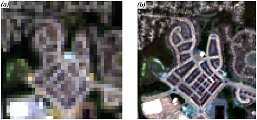
With the development of space-borne remote sensing instruments, high volumes of data on Earth surface processes have become available (Du et al. 2019; Kerner et al. 2019; Saha, Bovolo, and Bruzzone 2020; Shi et al. 2021; Wu et al. 2021). Remote sensing captures consistent information on a global scale across various spectral bands and provides new opportunities to monitor spatial and temporal patterns in urban areas change across the globe and across time. Owing to its long-term data record Landsat represents an obvious choice to monitoring long-term urban area changes at 30-m spatial resolution (Estoque and Murayama 2015; Liu et al. 2020; Sexton et al. 2013; Sinha, Verma, and Ayele 2016; Song et al. 2018; Song et al. 2016; Xue et al. 2014). Sexton et al. (2013) took advantage of Landsat time-series to monitor growing urban area changes for the Washington DC–Baltimore metropolitan area from 1984 to 2010. Song et al. (2018) used Landsat images over the same region to derive when and where urban impervious cover appeared from 1984 to 2010. Xue et al. (2014) used a time-series of Landsat imagery to develop an enhanced methodology that can identify the spatial dynamics of urban sprawl. Liu et al. (2020) leveraged Landsat time-series at a global scale to characterize the spatial pattern of urban area changes from 1985 to 2015. While Landsat allows the detection of changes going back to 1970s, not all changes can be detected at 30-m. With higher spatial and higher spectral resolution remote sensing data beginning to appear, more detailed LCLU information can be extracted and utilized. The Copernicus Sentinel-2 mission, operated by the European Space Agency (ESA), demonstrates improvement over Landsat with higher temporal resolution (a revisit time of five days at the equator with cloud-free pixels) and higher spatial resolution monitoring (at 10–20 m). Sentinel-2 data is available globally from 2015 to the present (Drusch et al. 2012). Figure 1 shows two images of the same residential community acquired by Landsat 8 (at 30 m) and Sentinel-2 (at 10 m) satellites. It shows improvements offered by Sentinel-2 imagery compared to Landsat 8-based imagery. Research indicates that the mapping products from Sentinel-2 performed remarkably higher in contrast to similar analyses that used Landsat imagery (Priem et al. 2019). Sentinel-2 images have been actively used for creating urban area-related products at better spatial resolution such as mapping settlements (Qiu et al. 2020), impervious surfaces (Lefebvre, Sannier, and Corpetti 2016; Xu, Liu, and Xu 2018), and detecting changes (Papadomanolaki, Vakalopoulou, and Karantzalos 2021; Pomente, Picchiani, and Del Frate 2018).

Figure 1. True-color imagery (spectral bands red, green and blue) of different resolutions for the same area in July 2018: (a) Landsat 8 imagery (at 30-m spatial resolution). (b) Sentinel-2 imagery (10 m).

Deep learning (DL) represents state-of-the-art in image processing and has recently shown great performance in satellite image processing (Ma et al. 2019; Yuan et al. 2020). Training and validation of DL models, however, require a lot of labeled data (sometimes referred as ground truth or reference data) that are not always available at global scale. Burke et al. (2021) argue that, while there is an abundant amount of unlabeled satellite imagery, the scarcity and unreliability of ground/reference data make both training and validation of DL models challenging and is one of the biggest problems of using DL to support sustainable development. At the same, more and more satellite benchmark datasets become available in open domain and offer labeled imagery that are commonly used for advancing methods and model inter-comparison (Cheng et al. 2020; Van Etten et al. 2021). These datasets offer potential to further provide mapping and land area estimation outside the coverage of the benchmark datasets. In this study, we aim to utilize the Sentinel-2-based benchmark dataset, Onera Satellite Change Detection (OSCD) (Daudt et al. 2018), to train a DL model and analyze its performance at local scale to map urban land use changes, estimate area of changes and provide characterization of changes. OSCD consists of Sentinel-2 image pairs with labeled urban area change from 2015 to 2018 across 24 locations. OSCD has been successfully used for benchmarking and developing new DL algorithms (Luo et al. 2020; Papadomanolaki, Vakalopoulou, and Karantzalos 2021; Reichstein et al. 2019; Saha et al. 2020; Zhan et al. 2020). However, existing works on OSCD were limited to urban area change mapping only without addressing the problems of area estimation and area change characterization. We trained a DL model based on the original FC-Siam-Diff architecture (Daudt et al. 2018) by incorporating a mixed cross-entropy and dice loss function to better reflect the shape of urban area changes. We evaluated not only the overall performance of the DL model but also for each location separately, because location-specific accuracy values influence the number of samples to be used for area estimation (Olofsson et al. 2014). We directly applied the model for our study area, Washington DC–Baltimore region, to estimate and characterize area of changes in 2018–2019. Stratified random sampling was employed for estimating the area of changes and characterization of changes, where strata were derived from change detection maps. The samples were labeled with not only change/no change labels, but also with transitions between different urban functions from 2018 to 2019 utilizing visual interpretation of very high spatial resolution (VHR) imagery available in Google Earth. The use of high-quality samples allowed us to derive unbiased estimates of areas of change, as well fine-grained characterization of changes.

The remainder of the manuscript is organized as follows. Section 2 introduces the data used in the study. Section 3 describes the methodology along with implementation details. Section 4 presents experimental results. Finally, conclusions are made in Section 5.

2. Study area: Washington DC–Baltimore region for independent validation

Our study area is within the Sentinel-2 tile 18SUJ, Washington DC–Baltimore MD region. The Washington DC area is 33.4 × 33.3 km² and covers completely DC and parts of Virginia and Maryland; while the Baltimore area is 38.4 × 30.7 km² and consists of Baltimore City and the surrounding area. According to the United States Census 2020, population in Washington DC has increased by 100,500 from 2010 to 2019 (16.6% increase). The top three most populous counties in Maryland, namely Montgomery County, Prince George’s County, and Baltimore County, increased their population by 75,100, 42,900, and 20,700 people, respectively, during the past decade. This trend contributes to a variety of urban area changes occurring in these regions. As one of the most educated, highest-income, and fourth-largest combined statistical areas in the United States, the Washington DC–Baltimore region has been experiencing rapid economic development. Integrated with economic and demographic data, changes arising in this local area are supposed to reflect the underlying socio-economic context.

Multiple studies have been conducted in this area, but most of them focused on monitoring urban change exploiting derived Landsat imagery at 30 m resolution, without taking high-spatial-resolution images into account (Masek, Lindsay, and Goward 2000; Sexton et al. 2013; Song et al. 2016). Therefore, the corresponding Sentinel-2 image pairs at 10 m resolution acquired in April 2018 and August 2019 over this region are provided for identifying and monitoring urban area change. It should be mentioned that apart from pixel-wise labels of change/no-change, sources of land use changes are generated for stratified samples manually. For example, whether the observed location was an active construction site or completed, and the type of buildings built (commercial, residential, school, hospital). For the false alarm cases, we also recorded the source of misclassifications. This post-analysis after getting binary change map is aimed to reveal the nature of urban area changes.

3. Data description

The following datasets are used in this study: OSCD dataset, a 18 × 18 km² fully labeled region which is part of Washington DC area, and large-scale Washington DC–Baltimore region for independent validation. All satellite images were acquired by the Multi-Spectral Instrument (MSI) aboard Sentinel-2A and Sentinel-2B satellites. The images contain 13 spectral bands at 10, 20, and 60 m spatial resolution with a 5-day revisit cycle (Pesaresi et al. 2016).

3.1. Open-sourced OSCD dataset for training

The OSCD dataset (Daudt et al. 2018) is a Sentinel-2-based imagery collection focused on urban area changes between 2015 and 2018. It provides labels for 24 locations around the world, including South America, North America, Europe, and Asia. Binary labels (change/no-change) are provided for each pixel. Fourteen training locations are Abu Dhabi (United Arab Emirates), Aguas Claras (Brazil), Beihai (China), Beirut (Lebanon), Bercy (France), Bordeaux (France), Cupertino (United States), Mumbai (India), Nantes (France), Paris (France), Pisa (Italy), Rennes (France), Hongkong (China), eastern Saclay (France). They cover dry tropical bare ground, dry tropical montane vegetation, sub-tropical montane vegetation, sub-tropical lowland vegetation, sub-tropical wetland, temperate lowland vegetation and temperate montane vegetation ecoregions (Hansen et al. 2022), which make the derived model more robust and flexible. The Washington DC is located in a temperate montane vegetation zone. Ten locations in the test dataset are also globally distributed: Brasilia (Brazil), Montpellier (France), Valencia (Spain), Norcia (Italy), Chongqing (China), Dubai (United Arab Emirates), Milano (Italy), Rio (Brazil), West Saclay (France), and Lavages (Canada). This dataset has been widely used in urban area change detection (Luo et al. 2020; Papadomanolaki, Vakalopoulou, and Karantzalos 2021; Saha et al. 2020; Zhan et al. 2020).

3.2. Fully labeled images of Washington DC for model evaluation

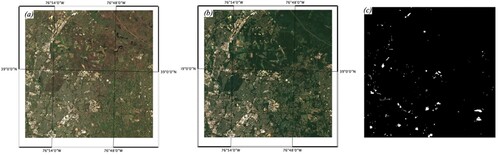
The second dataset, which is independent from OSCD, is part of the Sentinel-2 tile 18SUJ, which covers the metropolitan area of Washington DC (Figure 2). The size of the area is 18 × 18 km² (or 1800-by-1800 px at 10-m resolution). Due to the rapid development and economical significance Washington DC and the surrounding areas have received much attention. Many urban area changes, including construction or alteration of residential and commercial properties, occur in this area. It is important to identify and analyze these changes in support of the development of this area. Bi-temporal Sentinel-2 images acquired in April 2018 and August 2019 were utilized in this study. Ground truth of Washington DC (pixel-wise change/no-change labels) was fully labeled by us to evaluate the robustness and effectiveness of the network model trained using OSCD data (Figure 2).

Figure 2. The true-color images and ground truth labels of changes in the Washington DC area: (a) Sentinel-2 image acquired on 26 April 2018; (b) 19 August 2019; (c) ground truth labels of identified urban changes.

4. Methodology

4.1. Image preprocessing

To facilitate the use of the OSCD-based classification models over different areas, we pre-processed Sentinel-2 data with the state-of-the-art algorithms: Land Surface Reflectance Code (LaSRC) for atmospheric correction (Doxani et al. 2018; Vermote et al. 2016) and multi-temporal co-registration (Skakun et al. 2017). The LaSRC-based atmospheric correction allows one to reduce the impact of the atmosphere on the signal reflected from the Earth to the sensor and derive bottom-of-atmosphere (BOA) reflectance (or surface reflectance). As such, all locations would exhibit the same physical values in the satellite imagery. Co-registration allows reaching a sub-pixel alignment of multi-temporal satellite images, which is important in change detection. In OSCD, we used nine spectral bands representing blue, green, red, red-edge (3 bands), near-infrared (NIR), and short-wave infrared (SWIR, 2 bands) wavelengths. Other bands, such as coastal blue, water vapor, and cirrus, were not utilized because they are mainly preserved for estimating atmospheric properties and cloud detection. All 20-m bands were resampled to 10-m resolution using the nearest neighborhood method (Moya et al. 2020).

The Sentinel-2 image pairs of the OSCD dataset were divided into the train (14 locations) and test sets (10 locations) by data providers (Daudt et al. 2018). We cropped each image pair into 256 × 256 px patches with a stride of 128 pixels, allowing overlapping areas between two adjacent image patches. To reduce model overfitting we implemented various techniques for data augmentation. We used classical techniques such as random rotations (multiples of 90°) and flipping (right/left, up/down). To augment image patches with changes, the following approach was applied: we took two images (at least one image describes an urban area), where one would be from one location and another one would be from a different location, so that pair would yield urban changes for all pixels. This was done to increase the proportion of pixels that were labeled with changes. After data augmentation, there are approximately 6.9 × 10⁶ changed pixels in the training dataset, accounting for 17.08% of all training pixels; approximately 1.1 × 10⁶ changed pixels exist in the test set, accounting for 5.17% of all testing image pixels.

Given that the range of surface reflectance values varies with wavelength, it is critical to normalize the data before inputting it into the network. The following equation was used for normalization: (1) $\mathrm{Normalized}=(\mathrm{Reflectance}-\mathrm{mean})/\mathrm{standard}\mathrm{deviation}$(1)

The mean and standard deviation are calculated for each band according to all images in each band for train data. The locations of OSCD data are from all around the world, making the normalization more robust. After applying mean and standard deviation to Equation (1), the obtained surface reflectance values were then input to the network.

Considering 18 × 18 km² labeled image of Washington DC for model evaluation and Washington DC–Baltimore region for independent validation, the Sentinel-2 images underwent the same processing steps of atmospheric correction and co-registration as OSCD dataset.

4.2. Model architecture

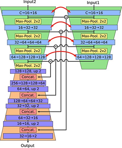
When building the model, the benchmark Fully Convolutional Siamese-Difference architecture (FC-Siam-Diff) (Daudt et al. 2018) was trained on the OSCD dataset. FC-Siam-Diff, as shown in Figure 3, is an improved algorithm based on U-net (Ronneberger, Fischer, and Brox 2015), including encoding and decoding layers. Assuming the image before and after changes have similar representation, the encoding layers of the FC-Siam-Diff consist of two identical streams with shared weights. Each image in one pair is then fed into one of these identical streams respectively, and the difference between the two images in the encoding layer is calculated. The obtained difference values are concatenated to the original decoding process by skip connection. This architecture emphasizes the difference between two image pairs, which is the change we pay more attention to.

Figure 3. The architecture of original FC-Siam-Diff (Daudt et al. 2018).

Training of the network is done through the minimization of the loss function. The cross-entropy loss function is widely used in deep learning models, especially for multi-classifier learning (Ma, Liu, and Qian 2004; Zhou et al. 2019). Compared to focal loss requiring more hyperparameters, the cross-entropy loss can achieve better performance with limited parameters. The formula of cross-entropy is as follows: (2) $L_{CE}=-\sum _{i=1}^n{t}_i\log (p_i)(\mathrm{for}n\mathrm{classes})$(2) where $t_i$ is the target label and $p_i$ is the neural network output.

However, there remain several fundamental problems. When the labels of each class are imbalanced, especially in change detection where training change pixels are limited, the training process tends to focus more on the dominant class (in this case no change). Therefore, a weighted cross-entropy loss function was used to assign a larger weight to changed pixels and a smaller weight to unchanged pixels to balance the contribution of each class: (3) $L_{\mathrm{weighted}\mathrm{\_}\mathrm{CE}}=-\sum _{i=1}^n{\alpha }_i{t}_i\log (p_i)$(3) where ${\alpha }_i\in [0,1]$ is inverse proportional to the class frequency (Ho and Wookey 2019). This is used in the original FC-Siam-Diff network. However, it should be noted that the cross-entropy loss suffers from limitations in our binary urban change detection field. The loss does not take commission error into consideration, because when $t_i$ = 0, $L_{CE}=0$ ignoring wrong detection of identifying true background as targets.

To consider commission error and omission error at the same time and deal with imbalanced data, we also included the dice loss component in the loss function. Dice loss is based on the Sørensen–Dice coefficient (Sørensen 1948), which is a measure of overlap and is widely used to assess the segmentation performance (Milletari, Navab, and Ahmadi 2016). The two-class variant of dice loss is expressed as: (4) $L_{\mathrm{dice}}=1\text{–}(2|A\cap B|)/(|A|+|B|)=1\text{–}2\mathrm{TP}/(2\mathrm{TP}+\mathrm{FP}+\mathrm{FN})$(4)

For the change detection case, A is the set that contains all predicted changed pixels, and B is the changed pixels labeled in the ground truth. TP, true positive, means the number of pixels that are correctly predicted as changes. FP, false positive, means the number of pixels that are incorrectly predicted as changes. And FN, false negative, refers to the number of pixels that the model wrongly predicted as non-changes. The dice loss could be used as a loss function to maximize the overlap between two sets and is more stable in the data-imbalance situations (Li et al. 2019).

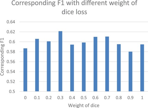
Consequently, a mixed dice loss and weighted cross-entropy loss was introduced as a loss function when training the modified FC-Siam-Diff in our research: (5) $\mathrm{mixed}=\propto \times L_{\mathrm{dice}}+(1-\propto )\times L_{\mathrm{weighted}\mathrm{\_}\mathrm{CE}}$(5) where ∝, (1–∝) represent the corresponding significance of dice loss and cross entropy loss. According to extensive experiments, ∝ = 0.3 was found to obtain a better performance in this case. All experiments related to modified FC-Siam-Diff were implemented using the PyTorch deep learning library on an NVIDIA Tesla V100 PCIe with 16 GB of GPU memory.

4.3. Comparison models

To select the best model for identifying urban area change and estimating areas, the modified FC-Siam-Diff was compared to other methods, assuming Chen et al. (2020) as a reference.

4.3.1. Multi-layer perceptron (MLP)-based algorithm

We compared the multi-layer perceptron-based algorithm (Zhang, Skakun, and Prudente 2020) to demonstrate the assumption that the utilized end-to-end neural network provides higher accuracy than the pixel-based post-classification algorithm.

Multi-layer perceptron (MLP) has been largely utilized and demonstrated its better performance in various applications, especially in land use and land cover mapping (Bhanage, Lee, and Gedem 2021). It consists of three layers of nodes – input layer, at least a hidden layer, and an output layer. Each node except those belonging to the input layer serves as a neuron and a nonlinear activation function is employed in each neuron. It can extract intricate patterns and recognize nonlinear relationships between various features. Nevertheless, neighboring information and spatial context are ignored considering its pixel-based conception.

In Zhang, Skakun, and Prudente (2020), change detection consisted of two major steps: mapping based on MLP and post-classification change detection based on classification results. Provided with hundred polygons and corresponding labels, MLP was trained to classify Sentinel-2 images in the Washington DC area for two time periods in 2018 and 2019. Considering the derived classification maps were labeled as urban area and non-urban area, the differences between the two classification maps served as the urban area change map.

4.3.2. L-Unet

L-Unet, an up-to-date and unique model based on the Unet backbone, was proposed recently, and tested by Papadomanolaki, Vakalopoulou, and Karantzalos (2021). The algorithm conducts integrated fully convolutional long short-term memory (LSTM) (Hochreiter and Schmidhuber 1997) blocks on top of each encoding layer, capable of simulating potential temporal relationships of spatial features. LSTM is a type of recurrent neural network (RNN) and is aimed at learning order dependence in sequence prediction problems, which makes it possible to capture temporal relationships between different dates. However, considering the loss function, the model merely utilizes the cross-entropy loss. This is one of the up-to-date algorithms utilized in change detection and serves as one comparison method to demonstrate the outperformance of our derived model with a more feasible loss function.

4.4. Performance assessment

4.4.1. Model evaluation

To quantitatively evaluate the model’s performance, three different evaluation metrics were employed, i.e. user’s accuracy (UA), producer’s accuracy (PA), and F1 score. TP, FP, FN have the same definition as in Equation (4). (6) $\mathrm{UA}=\mathrm{TP}/(\mathrm{TP}+\mathrm{FP})$(6) (7) $\mathrm{PA}=\mathrm{TP}/(\mathrm{TP}+\mathrm{FN})$(7) (8) $F1=(2\times \mathrm{UA}\times \mathrm{PA})/(\mathrm{UA}+\mathrm{PA})$(8)

4.4.2. Independent validation: area estimation and uncertainty quantification

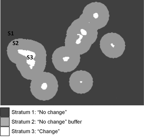
When monitoring urban changes, estimating the area of change (which is a different task of pure mapping) and its characterization is extremely important. Direct use of maps for estimating areas can lead to biases in estimations because of commission and omission errors (Gallego 2004). However, complete labeling of all changes in the DC and Baltimore areas (like it was done for the OSCD and DC locations) was not feasible and would be time and resource consuming. Therefore, a sample-based approach was adopted for estimating accuracies, areas of change and corresponding uncertainties. For this, we followed recommended protocols for land cover land use change (Olofsson et al. 2014; Olofsson et al. 2020). Stratified random sampling was employed, where strata were derived from change detection maps. Because in our case the area of no change would account for >99% of the total area the corresponding weight would influence the derived uncertainties of area estimates (for example, see Equation (10) in Olofsson et al. (2014)) – the larger the stratum weight, the more considerable uncertainties of estimated areas of change. Therefore, a spatial buffer of 20 pixels (at 10 m) was introduced to include areas of no change around areas of change. The main goal of introducing the buffer was to mitigate the effects of omission errors which would lead to large uncertainties in change area assessment (Olofsson et al. 2020). The 20-pixel size of the buffer was selected following recommendations outlined in Olofsson et al. (2020). Figure 4 shows an example of three strata used.

Figure 4. Illustration of three strata used in the sample-based approach for accuracy assessment and area estimation.

Overall, 500 samples were used for each location (DC and Baltimore), with 100 samples allocated for the change stratum, 100 samples for the buffer stratum, and the rest 300 samples allocated for the no-change stratum. In terms of responsive design, a 10-m pixel was selected as an elementary sampling unit. The reference data source was very high spatial resolution imagery available in Google Earth with the time period overlapping with the Sentinel-2 images used in this study. During the labeling process, we labeled samples with change or no change class and the type of change, for example, whether the observed location was an active construction site or completed, and the type of buildings built (commercial, residential, school, hospital). For the false alarm cases, we also recorded the source of misclassifications. Based on the samples we calculated producer’s and user’s accuracies and areas of change along with corresponding uncertainties using equations from Olofsson et al. (2014).

5. Results and discussion

In this section, we describe the performance of the deep learning model on the OSCD test dataset, 18 × 18 km² labeled Washington DC images, and independent Washington DC–Baltimore images. The samples in the latter are also used to characterize urban changes occurring in the Washington DC–Baltimore area.

5.1. OSCD dataset

Table 1 shows the performance metrics of the trained model for ten locations available in the OSCD test data. User’s accuracy (UA), producer’s accuracy (PA), and F1 score vary significantly in terms of location. For example, the network yielded the best performance for the Montpellier (France) site achieving 75.72%, 72.92%, and 74.30% for UA, PA, and F1 scores, respectively. Performance of the network for the Valencia (Spain) site was much worse, yielding accuracies of 4.94%, 6.77%, and 5.71% for UA, PA, and F1 score. That region features very few changes and most of those changes were small and could not be detected at Sentinel-2 10-m resolution. We consider that the mislabeling in the OSCD dataset is supposed to account for the worse performance. As shown in Figure 5, several inaccurate labels exist in both train and test data of the OSCD. The description of OSCD depicts that the annotated changes pay attention to urban changes. But some boats near the seashore which should not be part of urban change are identified as urban changed pixels. Meanwhile, some constructed buildings which are supposed to be urban area changes are missing. Therefore, the inferior performance in Valencia may result from those wrong labels to some extent.

Figure 5. Labels in the OSCD dataset not relevant to urban changes. The top row is urban change, which is not labeled, and the bottom row shows boats, which are mislabeled as urban change.

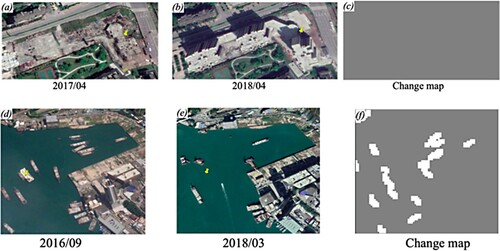
Table 1. Evaluation metrics for each test location in OSCD.

Location	UA	PA	F1
Montpellier	75.72	72.92	74.30
Las Vegas	72.85	74.53	73.68
Rio	60.51	67.06	63.62
Chongqing	69.30	51.58	59.14
Dubai	61.00	53.86	57.21
Brasilia	79.16	42.52	55.32
Milano	62.62	38.74	47.86
Saclay_w	39.97	48.49	43.82
Norcia	50.69	25.46	33.90
Valencia	4.94	6.77	5.71
Average	57.68	48.19	51.46

It should be mentioned that different weights between cross-entropy and dice coefficient loss in the loss function (Equation 5) led to slightly different performance, as illustrated in Figure 6. ∝ = 0 expressed merely cross-entropy was used as loss function, leading to lower performance compared to adding dice loss. At the same time, our experiments showed that ∝ = 0.3 yielded the best results. Overall, performance in terms of F1 score varied non-linearly depending on the weight values ∝.

Figure 6. Dependence of the F1 score on the ∝ coefficient in the loss function (Equation 5) obtained for the OSCD test data.

Performance of the modified FC-Siam-Diff model in the OSCD dataset is also compared to two networks: the original network, where a weighted cross entropy loss function is used (Daudt et al. 2018), and one of the state-of-art networks, which uses a time-series of Sentinel-2 images to predict urban changes (Papadomanolaki, Vakalopoulou, and Karantzalos 2021). Table 2 illustrates model performance for all test locations.

Table 2. Evaluation metrics for different methods in OSCD.

Method	UA	PA	F1
Original FC-Siam-Diff (Daudt et al. 2018)	57.84	57.99	57.92
L-Unet (Papadomanolaki, Vakalopoulou, and Karantzalos 2021)	54.29	63.05	58.34
Our model (this work)	65.89	60.20	62.91

Our model with a mixed loss function outperforms the original version with the UA exceeding 8.05%, PA exceeding 2.21%, and overall F1 score exceeding 4.99%, meaning that the mixed loss function handles the imbalanced problem well and identifies urban area changes more accurately. Both higher UA and PA values indicate our derived change detection map is relatively reliable and accurate in contrast to the original version. Even though the PA is lower than the network proposed by Papadomanolaki, Vakalopoulou, and Karantzalos (2021), the higher UA (11.6% higher) and F1 score (4.57% higher) shows our model is capable of minimizing the underestimation and reinforcing the credibility of the change map and area estimation.

5.2. Labeled Washington DC area

The developed network was also applied to the 18 × 18 km² fully labeled Washington DC images with the derived change map as shown in Figure 7. The red polygons are ground truth, which was manually labeled, and the white pixels are change pixels predicted by the network. Figure 7 shows a significant number of urban area changes occurred from 2018 to 2019, especially in the southwest part of the DC area. For better qualitative evaluation, three areas are highlighted in the Washington DC area as shown in Figure 7. Buildings constructed from 2018 to 2019 can be seen, and the identified boundaries match the ground truth relatively well. For quantitative valuation, all metrics are summarized in Table 3 with a UA of 76.01%, PA of 31.39%, and F1 score of 44.43%. This indicates that 76.01% of these predicted change pixels are real urban change, and 31.39% change pixels in ground truth are identified for the Washington DC area. The omission errors are mainly due to the small size of urban changes that cannot be distinguished with 10-m Sentinel-2 imagery.

Figure 7. (a) The change map from MLP-based algorithm. (b) The change map from our network, the white pixels are the changed area detected by the network and the red polygons are the ground truth we labeled. (c) Three areas are zoomed in to describe the urban area change in the derived change map based on our network.

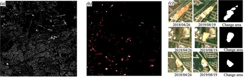
Table 3. Evaluation metrics for different methods in 18 × 18 km² labeled DC.

Model	UA	PA	F1
MLP (Zhang, Skakun, and Prudente 2020)	3.21	23.87	5.66
DL (this work)	76.01	31.39	44.43

We compared the derived end-to-end neural network with our previous work, pixel-based post-classification algorithm described in section 3.4.1 in the Washington DC area (Figure 7). The pixel-based classification does not account for spatial context and, therefore, the produced map features a ‘salt and pepper’ noise. As shown in Table 3, the UA is 3.21%, and the F1 score is 5.66%, substantially lower than the network we utilized. The main reason is owing to the superiority of the similar U-net architecture, which takes the neighboring information of each pixel into consideration.

5.3. Washington DC–Baltimore region

5.3.1. Change detection map

Figure 8 shows the derived change detection maps for the large Washington DC and the Baltimore areas, while Table 4 shows the derived PA and UA along with estimated areas of urban changes using a sample-based approach. The sample-based approach allowed us to derive unbiased estimates of accuracy values and areas along with corresponding uncertainties (see Equations 5–7 in Olofsson et al. (2014)). The estimated accuracies are in correspondence to the accuracies obtained for the fully labeled subset of the DC area with PA for the Baltimore location almost twice higher. Overall, the area of changes during the April 2018–August 2019 time period was estimated at 10.9 ± 4.3 km² (0.85% of the total area) and 10.8 ± 2.2 km² (0.92%) for DC and Baltimore areas, respectively.

Figure 8. (a, c) Sentinel-2 images for large DC area and Baltimore area attained in August 2019. (b, d) The derived change map for the large DC area and Baltimore area from April 2018 to August 2019.

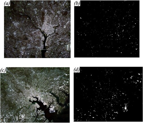
Table 4. Accuracies of change detection maps for the DC and Baltimore areas derived using a sample-based approach. Uncertainties are expressed as 1 standard error (SE).

	Washington DC	Baltimore
PA, %	40.24 ± 15.91	73.10 ± 13.90
UA, %	63.00 ± 4.85	57.00 ± 4.98
Area of changes, km^2 (relative to the total area, %)	10.9 ± 4.3 (0.85)	10.8 ± 2.2 (0.92)

Combining derived urban area change map with U.S. County boundary, we found that there were 18,576 urban area changed pixels (at 10 m) in Washington D.C., accounting for around 1.05% of the whole city, while 28,202 pixels happened urban changes in Baltimore city, accounting for 1.26% of the entire city. At the same time, the detected urban changed pixels in Alexandria (VA) reached 2667 pixels, accounting for about 0.66% of the county.

As shown in Figure 9, in contrast to the conclusion in Song et al. (2016) that the expansion of built-up areas in the DC-Baltimore metropolitan region was highly concentrated along major highways, our map shows the main urban changes from 2018 to 2019 did not show obvious aggregation along primary highways. The changes express more disperse distribution.

Figure 9. Urban change map with primary roads (https://www.census.gov/geographies/mapping-files.html).

It is worth mentioning that the relationship between urban population growth and urban area change detection is also taken into account for further analysis. According to statistic data of population growth from U.S. Census data (https://www.census.gov/popest), the rate of population growth in Alexandria is 0.97% exceeding the urban change rate. In contrast to the conclusion in Song et al. (2016), the rate of population growth consistently exceeded the rate of impervious expansion from 1985 to 2010 for most municipalities, the pattern in Alexandria (VA) keeps consistent. Nevertheless, the population growth rate in Washington D.C. is nearly 0.67%, lower than the urban area change rate. In addition, the opposite was found in Baltimore city that the population decreases 1.49% from 2018 to 2019, demonstrating that population growth is not only the underlying driving force of urban changes. According to the visual interpretation of urban changes, more facilities built-up like schools and airport expansion explained part of urban dynamics, illustrating economic, social, political, and environmental factors contribute to urban area change.

5.3.2. Post-classification analysis of land use

Post-classification analysis of land use, associated with transitions between various urban functions, is generated for stratified samples manually. It was found that among detected changes, active constructions (those that can be seen in the 2019 imagery) accounted for 78% and 86% in DC and Baltimore, respectively, while the rest represented the completed constructions. Commercial buildings accounted for 52% (DC) and 46% (Baltimore), and residential buildings accounted for 27% and 21%. Worth noting that approximately 8–9% of detected changes in DC and Baltimore occurred due to the construction of new schools or renovation of existing ones. This high number illustrates more attention was paid to education, as such overcrowded school buildings require renovations. Another type of change identified was the construction of parking lots next to commercial buildings, roads, and hospitals.

In terms of commission errors, the majority (57% in DC and 30% in Baltimore) of those misclassifications were due to changes in the façade of buildings, specifically roofs (either repainted or installation of solar panels). Other sources of false change detection were mining, recycling, waste, and landfill facilities that accounted for 19% (DC) and 33% (Baltimore); boundaries of changes (over-segmentation) (16% and 5%); changes in the bare ground or water (e.g. boats) (8% and 14%); and agricultural (0% and 12%) (Figure 10).

Figure 10. (a) Two detected urban changes in the independent DC area are highlighted. (b) Two detected urban changes in the independent Baltimore area are highlighted. (c) False alarm pixels related to fields in the DC area.

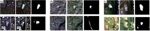
Missed areas of change (omission errors) were due to the spatial resolution of Sentinel-2 images at 10 m and were mainly small-area constructions with areas ranging from 200 m² (2 pixels) to 800 m² (8 pixels). Compared to identify urban changes in 30-m by 30-m grid (Song et al. 2016), Sentinel-2 shows its ability to detect fine-grain changes due to its 10-m spatial resolution.

6. Conclusions

In this study, we addressed the problem of leveraging the use of labeled datasets (namely OSCD) for not only mapping urban changes from 10-m Sentinel-2 imagery, but also estimating the area of change and characterizing types of changes. Though the location-averaged PA and UA accuracy values on the OSCD dataset were 48.2% and 57.7%, respectively, and direct application of maps would yield biased estimates of areas, we showed that a statistically rigorous approach through sampling allows one to obtain unbiased estimates. Furthermore, fine-grain labels of samples regarding land use changes allowed us to perform a more fine-grained analysis. In particular, an OSCD-trained deep learning neural network was directly applied to Sentinel-2 imagery acquired in 2018–2019 over the Washington DC–Baltimore area. The derived map was used as a ‘guidance’ tool (through stratification) to provide high-quality samples, which were labeled using VHR satellite data available in Google Earth. Our results showed that approximately 1% of the Washington DC–Baltimore area underwent changes with the majority being the construction of commercial buildings (45–55%) followed by residential buildings (20–30%). A sample-based approach also allowed us to identify sources of errors in the maps, such as small constructions (omission errors), and agricultural areas and landfills (commission errors). To mitigate the former satellite images with a better spatial resolution could be applied (e.g. Planet at 3 m); to mitigate the latter multi-temporal features derived from Sentinel-2 time-series should be employed, along with other potential data sources, such as synthetic aperture radar (SAR). Based on this research, it is also worth noticing that enhancing the training data is one of the problems to be addressed in future studies. And mapping urban area changes all around the world will be inspiring. These will constitute future research directions. Overall, we think that this study makes important contributions by demonstrating the utility of benchmark datasets not only for developing and comparing image processing algorithms but for serving as a foundation for creating relevant global satellite-derived products.

Disclosure statement

No potential conflict of interest was reported by the author(s).

Data availability statement

The data OSCD that support the findings of this study are openly available in IEEEDataPort at http://doi.org/10.21227/asqe-7s69. The data of small Washington DC datasets, and large Washington DC–Baltimore area that support the findings of this study are available from Yiming Zhang, [YZ], upon reasonable request.

Additional information

Funding

This research is based upon work supported in part by the Office of the Director of National Intelligence (ODNI), Intelligence Advanced Research Projects Activity (IARPA) [Contract Number 2021-20111000005], and NASA Land-Cover/Land-Use Change (LCLUC) Program [grant number 80NSSC21K0314].

References

- Bhanage, V., H. S. Lee, and S. Gedem. 2021. “Prediction of Land Use and Land Cover Changes in Mumbai City, India, Using Remote Sensing Data and a Multilayer Perceptron Neural Network-Based Markov Chain Model.” Sustainability 13 (2): 471. doi:10.3390/su13020471.
- Burke, M., A. Driscoll, D. B. Lobell, and S. Ermon. 2021. “Using Satellite Imagery to Understand and Promote Sustainable Development.” Science 371 (6535): eabe8628. doi:10.1126/science.abe86.
- Chen, T. H. K., C. Qiu, M. Schmitt, X. Zhu, C. E. Sabel, and A. V. Prishchepov. 2020. “Mapping Horizontal and Vertical Urban Densification in Denmark with Landsat Time-Series from 1985 to 2018: A Semantic Segmentation Solution.” Remote Sensing of Environment 251: 112096. doi:10.1016/j.rse.2020.112096.
- Cheng, G., X. Xie, J. Han, L. Guo, and G. S. Xia. 2020. “Remote Sensing Image Scene Classification Meets Deep Learning: Challenges, Methods, Benchmarks, and Opportunities.” IEEE Journal of Selected Topics in Applied Earth Observations and Remote Sensing 13: 3735–3756. doi:10.1109/JSTARS.2020.3005403.
- Cowen, D. J., and J. R. Jensen. 1998. “Extraction and Modeling of Urban Attributes Using Remote Sensing Technology.” In People and Pixels: Linking Remote Sensing and Social Science, edited by Diana Liverman, Moran Emilio, Rindfuss Ronald, and Stern Paul, 164–188. Washington, DC: National Academy Press.
- Daudt, R. C., L. B. Saux, B. Alexandre, and Y. Gousseau. 2018. “Urban Change Detection for Multispectral Earth Observation Using Convolutional Neural Networks.” In Proceedings of the IEEE International Geoscience and Remote Sensing Symposium (IGARSS), 2115–2118. IEEE. doi:10.1109/IGARSS.2018.8518015.
- Deilami, K., M. Kamruzzaman, and Y. Liu. 2018. “Urban Heat Island Effect: A Systematic Review of Spatio-Temporal Factors, Data, Methods, and Mitigation Measures.” International Journal of Applied Earth Observation and Geoinformation 67: 30–42. doi:10.1016/j.jag.2017.12.009.
- DESA, U. 2019. World Urbanization Prospects: The 2018 Revision (ST/ESA/SER. A/420). New York: United Nations.
- Doxani, G., E. Vermote, J. C. Roger, F. Gascon, S. Adriaensen, D. Frantz, O. Hagolle, et al. 2018. “Atmospheric Correction Inter-Comparison Exercise.” Remote Sensing 10 (2): 352. doi:10.3390/rs10020352.
- Drusch, M., U. D. Bello, S. Carlier, O. Colin, V. Fernandez, F. Gascon, B. Hoersch, et al. 2012. “Sentinel-2: ESA's Optical High-Resolution Mission for GMES Operational Services.” Remote Sensing of Environment 120 (15): 25–36. doi:10.1016/j.rse.2011.11.026.
- Du, B., L. Ru, C. Wu, and L. Zhang. 2019. “Unsupervised Deep Slow Feature Analysis for Change Detection in Multi-Temporal Remote Sensing Images.” IEEE Transactions on Geoscience and Remote Sensing 57 (12): 9976–9992. doi:10.1109/TGRS.2019.2930682.
- Estoque, R. C., and Y. Murayama. 2015. “Classification and Change Detection of Built-Up Lands from Landsat-7 ETM+ and Landsat-8 OLI/TIRS Imageries: A Comparative Assessment of Various Spectral Indices.” Ecological Indicators 56: 205–217. doi:10.1016/j.ecolind.2015.03.037.
- Foley, J. A., R. DeFries, G. P. Asner, C. Barford, G. Bonan, S. R. Carpenter, E. S. Chapin, et al. 2005. “Global Consequences of Land Use.” Science 309 (5734): 570–574. doi:10.1126/science.1111772.
- Gallego, F. J. 2004. “Remote Sensing and Land Cover Area Estimation.” International Journal of Remote Sensing 25 (15): 3019–3047. doi:10.1080/01431160310001619607.
- Gong, J., H. Sui, G. Ma, and Q. Zhou. 2008. “A Review of Multi-Temporal Remote Sensing Data Change Detection Algorithms.” The International Archives of the Photogrammetry, Remote Sensing and Spatial Information Sciences 37 (B7): 757–762.
- Hansen, M. C., P. V. Potapov, A. H. Pickens, A. Tyukavina, A. Hernandez-Serna, V. Zalles, S. Turubanova, et al. 2022. “Land Use Extent and Dispersion within Natural Land Cover Using Landsat Data.” Environmental Research Letters 17 (3): 034050. doi:10.1088/1748-9326/ac46ec.
- Ho, Y., and S. Wookey. 2019. “The Real-World-Weight Cross-Entropy Loss Function: Modeling the Costs of Mislabeling.” IEEE Access 8: 4806–4813. doi:10.1109/ACCESS.2019.2962617.
- Hochreiter, S., and J. Schmidhuber. 1997. “Long Short-Term Memory.” Neural Computation 9 (8): 1735–1780. doi:10.1162/neco.1997.9.8.1735.
- Kerner, H. R., K. L. Wagstaff, B. D. Bue, P. C. Gray, J. F. Bell, and H. B. Amor. 2019. “Toward Generalized Change Detection on Planetary Surfaces with Convolutional Autoencoders and Transfer Learning.” IEEE Journal of Selected Topics in Applied Earth Observations and Remote Sensing 12 (10): 3900–3918. doi:10.1109/JSTARS.2019.2936771.
- Lefebvre, A., C. Sannier, and T. Corpetti. 2016. “Monitoring Urban Areas with Sentinel-2A Data: Application to the Update of the Copernicus High Resolution Layer Imperviousness Degree.” Remote Sensing 8 (7): 606. doi:10.3390/rs8070606.
- Li, X., X. Sun, Y. Meng, J. Liang, F. Wu, and J. Li. 2019. “Dice Loss for Data-Imbalanced NLP Tasks.” ArXiv Preprint. http://arxiv.org/abs/1911.02855.
- Liu, X., Y. Huang, X. Xu, X. Li, X. Li, P. Ciais, P. Lin, et al. 2020. “High-Spatiotemporal-Resolution Mapping of Global Urban Change from 1985 to 2015.” Nature Sustainability 3 (7): 564–570. doi:10.1038/s41893-020-0521-x.
- Luo, X., X. Li, Y. Wu, W. Hou, M. Wang, Y. Jin, and W. Xu. 2020. “Research on Change Detection Method of High-Resolution Remote Sensing Images Based on Subpixel Convolution.” IEEE Journal of Selected Topics in Applied Earth Observations and Remote Sensing 14: 1447–1457. doi:10.1109/JSTARS.2020.3044060.
- Ma, Y., Q. Liu, and Z. Qian. 2004. “Automated Image Segmentation Using Improved PCNN Model Based on Cross-Entropy.” Paper Presented at Proceedings of 2004 International Symposium on Intelligent Multimedia, Video and Speech Processing, Hong Kong, October 20–22.
- Ma, L., Y. Liu, X. Zhang, Y. Ye, G. Yin, and B. A. Johnson. 2019. “Deep Learning in Remote Sensing Applications: A Meta-Analysis and Review.” ISPRS Journal of Photogrammetry and Remote Sensing 152: 166–177. doi:10.1016/j.isprsjprs.2019.04.015.
- Masek, J. G., F. E. Lindsay, and S. N. Goward. 2000. “Dynamics of Urban Growth in the Washington DC Metropolitan Area, 1973–1996, from Landsat Observations.” International Journal of Remote Sensing 21 (18): 3473–3486. doi:10.1080/014311600750037507.
- Milletari, F., N. Navab, and S. A. Ahmadi. 2016. “V-Net: Fully Convolutional Neural Networks for Volumetric Medical Image Segmentation.” Paper Presented at 2016 Fourth International Conference on 3D Vision (3DV), Stanford, CA, October 25–28.
- Moya, L., A. Muhari, B. Adriano, S. Koshimura, E. Mas, L. R. Marval-Perez, and N. Yokoya. 2020. “Detecting Urban Changes Using Phase Correlation and ℓ1-Based Sparse Model for Early Disaster Response: A Case Study of the 2018 Sulawesi Indonesia Earthquake-Tsunami.” Remote Sensing of Environment 242: 111743. doi:10.1016/j.rse.2020.111743.
- Olofsson, P., P. Arévalo, A. B. Espejo, C. Green, E. Lindquist, R. E. McRoberts, and M. J. Sanz. 2020. “Mitigating the Effects of Omission Errors on Area and Area Change Estimates.” Remote Sensing of Environment 236: 111492. doi:10.1016/j.rse.2019.111492.
- Olofsson, P., G. M. Foody, M. Herold, S. V. Stehman, C. E. Woodcock, and M. A. Wulder. 2014. “Good Practices for Estimating Area and Assessing Accuracy of Land Change.” Remote Sensing of Environment 148: 42–57. doi:10.1016/j.rse.2014.02.015.
- Papadomanolaki, M., M. Vakalopoulou, and K. Karantzalos. 2021. “A Deep Multitask Learning Framework Coupling Semantic Segmentation and Fully Convolutional LSTM Networks for Urban Change Detection.” IEEE Transactions on Geoscience and Remote Sensing 59 (9): 7651–7668. doi:10.1109/TGRS.2021.3055584.
- Pérez-Sindín, X. S., T. H. K. Chen, and A. V. Prishchepov. 2021. “Are Night-Time Lights a Good Proxy of Economic Activity in Rural Areas in Middle and Low-Income Countries? Examining the Empirical Evidence from Colombia.” Remote Sensing Applications: Society and Environment 24: 100647. doi:10.1016/j.rsase.2021.100647.
- Pesaresi, M., C. Corbane, A. Julea, A. J. Florczyk, V. Syrris, and P. Soille. 2016. “Assessment of the Added-Value of Sentinel-2 for Detecting Built-Up Areas.” Remote Sensing 8 (4): 299. doi:10.3390/rs8040299.
- Pomente, A., M. Picchiani, and F. Del Frate. 2018. “Sentinel-2 Change Detection Based on Deep Features.” In Proceedings of the 2018 IEEE International Geoscience and Remote Sensing Symposium, 6859–6862. IEEE. doi:10.1109/IGARSS.2018.8519195.
- Priem, F., A. Okujeni, S. van der Linden, and F. Canters. 2019. “Comparing Map-Based and Library-Based Training Approaches for Urban Land-Cover Fraction Mapping from Sentinel-2 Imagery.” International Journal of Applied Earth Observation and Geoinformation 78: 295–305. doi:10.1016/j.jag.2019.02.003.
- Qiu, C., M. Schmitt, C. Geiß, T. H. K. Chen, and X. X. Zhu. 2020. “A Framework for Large-Scale Mapping of Human Settlement Extent from Sentinel-2 Images via Fully Convolutional Neural Networks.” ISPRS Journal of Photogrammetry and Remote Sensing 163: 152–170. doi:10.1016/j.isprsjprs.2020.01.028.
- Reba, M., and K. C. Seto. 2020. “A Systematic Review and Assessment of Algorithms to Detect, Characterize, and Monitor Urban Land Change.” Remote Sensing of Environment 242: 111739. doi:10.1016/j.rse.2020.111739.
- Reichstein, M., G. Camps-Valls, B. Stevens, M. Jung, J. Denzler, and N. Carvalhais. 2019. “Deep Learning and Process Understanding for Data-Driven Earth System Science.” Nature 566 (7743): 195–204. doi:10.1038/s41586-019-0912-1.
- Ronneberger, O., P. Fischer, and T. Brox. 2015. “U-Net: Convolutional Networks for Biomedical Image Segmentation.” Paper Presented at the International Conference on Medical Image Computing and Computer-Assisted Intervention, Cham, October.
- Saha, S., F. Bovolo, and L. Bruzzone. 2020. “Building Change Detection in VHR SAR Images via Unsupervised Deep Transcoding.” IEEE Transactions on Geoscience and Remote Sensing 59 (3): 1917–1929. doi:10.1109/TGRS.2020.3000296.
- Saha, S., Y. T. Solano-Correa, F. Bovolo, and L. Bruzzone. 2020. “Unsupervised Deep Transfer Learning-Based Change Detection for HR Multispectral Images.” IEEE Geoscience and Remote Sensing Letters 18 (5): 856–860. doi:10.1109/LGRS.2020.2990284.
- Sexton, J. O., X. P. Song, C. Huang, S. Channan, M. E. Baker, and J. R. Townshend. 2013. “Urban Growth of the Washington, DC–Baltimore, MD Metropolitan Region from 1984 to 2010 by Annual, Landsat-Based Estimates of Impervious Cover.” Remote Sensing of Environment 129: 42–53. doi:10.1016/j.rse.2012.10.025.
- Shi, Q., M. Liu, S. Li, X. Liu, F. Wang, and L. Zhang. 2021. “A Deeply Supervised Attention Metric-Based Network and an Open Aerial Image Dataset for Remote Sensing Change Detection.” IEEE Transactions on Geoscience and Remote Sensing 60: 5604816. doi:10.1109/TGRS.2021.3085870.
- Sinha, P., N. K. Verma, and E. Ayele. 2016. “Urban Built-up Area Extraction and Change Detection of Adama Municipal Area Using Time-Series Landsat Images.” International Journal of Advanced Remote Sensing and GIS 5 (8): 1886–1895.
- Skakun, S., J. C. Roger, E. F. Vermote, J. G. Masek, and C. O. Justice. 2017. “Automatic Sub-Pixel Co-Registration of Landsat-8 Operational Land Imager and Sentinel-2A Multi-Spectral Instrument Images Using Phase Correlation and Machine Learning Based Mapping.” International Journal of Digital Earth 10 (12): 1253–1269. doi:10.1080/17538947.2017.1304586.
- Song, X. P., M. C. Hansen, S. V. Stehman, P. V. Potapov, A. Tyukavina, E. F. Vermote, and J. R. Townshend. 2018. “Global Land Change from 1982 to 2016.” Nature 560 (7720): 639–643. doi:10.1038/s41586-018-0411-9.
- Song, X. P., J. O. Sexton, C. Huang, S. Channan, and J. R. Townshend. 2016. “Characterizing the Magnitude, Timing and Duration of Urban Growth from Time Series of Landsat-Based Estimates of Impervious Cover.” Remote Sensing of Environment 175: 1–13. doi:10.1016/j.rse.2015.12.027.
- Sørensen, T. J. 1948. “A Method of Establishing Groups of Equal Amplitude in Plant Sociology Based on Similarity of Species Content and Its Application to Analyses of the Vegetation on Danish Commons.” Biologiske Skrifter 5: 1–34.
- Van Etten, A., D. Hogan, J. M. Manso, J. Shermeyer, N. Weir, and R. Lewis. 2021. “The Multi-Temporal Urban Development Spacenet Dataset.” In Proceedings of the IEEE/CVF Conference on Computer Vision and Pattern Recognition, 6398–6407. IEEE. doi:10.1109/CVPR46437.2021.00633.
- Vermote, E., C. Justice, M. Claverie, and B. Franch. 2016. “Preliminary Analysis of the Performance of the Landsat 8/OLI Land Surface Reflectance Product.” Remote Sensing of Environment 185: 46–56. doi:10.1016/j.rse.2016.04.008.
- Wu, C., H. Chen, B. Du, and L. Zhang. 2021. “Unsupervised Change Detection in Multitemporal VHR Images Based on Deep Kernel PCA Convolutional Mapping Network.” IEEE Transactions on Cybernetics. doi:10.1109/TCYB.2021.3086884.
- Xian, G., H. Shi, J. Dewitz, and Z. Wu. 2019. “Performances of WorldView 3, Sentinel 2, and Landsat 8 Data in Mapping Impervious Surface.” Remote Sensing Applications: Society and Environment 15: 100246. doi:10.1016/j.rsase.2019.100246.
- Xu, R., J. Liu, and J. Xu. 2018. “Extraction of High-Precision Urban Impervious Surfaces from Sentinel-2 Multispectral Imagery via Modified Linear Spectral Mixture Analysis.” Sensors 18 (9): 2873. doi:10.3390/s18092873.
- Xue, X., H. Liu, X. Mu, and J. Liu. 2014. “Trajectory-Based Detection of Urban Expansion Using Landsat Time Series.” International Journal of Remote Sensing 35 (4): 1450–1465. doi:10.1080/01431161.2013.878058.
- Ying, Q., M. C. Hansen, P. V. Potapov, A. Tyukavina, L. Wang, S. V. Stehman, R. Moore, and M. Hancher. 2017. “Global Bare Ground Gain from 2000 to 2012 Using Landsat Imagery.” Remote Sensing of Environment 194: 161–176. doi:10.1016/j.rse.2017.03.022.
- Yuan, Q., H. Shen, T. Li, Z. Li, S. Li, Y. Jiang, H. Xu, et al. 2020. “Deep Learning in Environmental Remote Sensing: Achievements and Challenges.” Remote Sensing of Environment 241: 111716. doi:10.1016/j.rse.2020.111716.
- Zhan, T., M. Gong, X. Jiang, and M. Zhang. 2020. “Unsupervised Scale-Driven Change Detection with Deep Spatial–Spectral Features for VHR Images.” IEEE Transactions on Geoscience and Remote Sensing 58 (8): 5653–5665. doi:10.1109/TGRS.2020.2968098.
- Zhang, Y., S. Skakun, and V. Prudente. 2020. “Detection of Changes in Impervious Surface Using Sentinel-2 Imagery.” In Proceedings of the 2020 IEEE International Geoscience and Remote Sensing Symposium on Remote Sensing, 4787–4790. IEEE. doi:10.1109/IGARSS39084.2020.9323327.
- Zheng, Z., Y. Zhong, J. Wang, A. Ma, and L. Zhang. 2021. “Building Damage Assessment for Rapid Disaster Response with a Deep Object-Based Semantic Change Detection Framework: From Natural Disasters to Man-Made Disasters.” Remote Sensing of Environment 265: 112636. doi:10.1016/j.rse.2021.112636.
- Zhou, Y., X. Wang, M. Zhang, J. Zhu, R. Zheng, and Q. Wu. 2019. “MPCE: A Maximum Probability Based Cross Entropy Loss Function for Neural Network Classification.” IEEE Access 7: 146331–146341. doi:10.1109/ACCESS.2019.2946264.