Mining hourly population dynamics by activity type based on decomposition of sequential snapshot data

ABSTRACT

The dynamic population distributions by activity type (e.g. working, shopping or in-home) are vital for resource allocation, urban planning and epidemic containment. Although studies have incorporated individual-level human mobility data to map population distribution by activity type, access to such data is hindered due to privacy issues and they rely on auxiliary data to provide priori activity knowledge. This paper presents a method for generating the population dynamics by activity type. We first introduce more readily available sequential snapshot data to construct the population mixture model, then decompose the population mixture, and finally estimate the dynamic population size for each activity. We test the method in the central districts of Guangzhou city, China, based on real-time Tencent user density data. Correlation analysis and accuracy assessment prove that our method can accurately estimate hourly distributions for populations engaging in working, stay-at-home, and socializing activities. The temporal distribution of the working population reproduces the regular work scenarios and socializing population displays complex spatial patterns. We also find that there is an underlying relationship between a region’s function and its dynamic population structure. The presented method has great potential for application and could provide new insight for studying urban dynamic functions.

KEYWORDS:

• Hourly population dynamics
• activity type
• population mixture model
• real-time Tencent user density data

1. Introduction

The pulses of cities are largely driven by human activity and human movement (Xu et al. 2018). Obtaining the population distributions by activity type, such as working, in-home, shopping or recreation, and understanding their dynamic change patterns can provide important data foundation for optimal resource allocation (Kang et al. 2020), epidemic containment (Mistry et al. 2021), disaster risk management (Bhaduri et al. 2007; Tatem et al. 2012; Song et al. 2019), urban and rural planning (Song et al. 2018; Huang et al. 2021), smart town construction (Shang et al. 2021; Song et al. 2021) and so on. For example, it can use to (1) improve the design and performance of urban spaces by exploring the correlations between population size by activity type and various urban features (e.g. land use or urban morphology) (Tu et al. 2017); (2) help urban planners and policy-makers to optimize resource allocation and improve facility allocation by quantifying differences in access to resources and facilities across activity-based population groups (Wu, Cheng, et al. 2020). Meanwhile, it also helps reveal the interaction mechanism among human activities, the ecological environment and spatial structure (Stevens et al. 2015; Yang et al. 2019; Xing et al. 2020), thus providing support for optimizing population management policies. However, due to a lack of data, few studies have focused on estimating the distribution of people engaging in different activities as opposed to studies estimating the distribution of the total population (Greger 2015; Hanaoka 2018; Park et al. 2020).

In recent years, the rapid development of mobile positioning and location-aware technologies has provided us with various individual mobility data with high spatial and temporal accuracy (e.g. mobile phone data and smart card data). The high penetration rate of mobile phones, which is still increasing, has made mobile phone data a valuable resource for mapping population distributions by activity type.

Existing studies mainly use two types of mobile phone data: individual trajectory data and sequential snapshot data. Studies based on individual trajectory data propose two different approaches. Some studies (Zhang, Zhou, and Zhang 2017; Wu, Wang, et al. 2020; Qian et al. 2021) first categorized cell phone users into different groups (e.g. residents, workers, commuters and tourists) according to their general behavioral characteristics extracted from the individual trajectory, i.e. where they stay, how often they appear at a certain place, and how long they stay there. The spatial distribution of different population groups can then be obtained by counting the number of cell phone users within the spatial aggregation units (e.g. grids, and traffic analysis zones). Scholar has used this approach to produce the spatial distribution of different types of populations and to analyse the spatiotemporal mobility patterns of certain population groups (Wu, Wang, et al. 2020). However, these population groups are often not categorized by activity types. It is, therefore, not possible to reveal the dynamic population distribution by activity type using this approach. Other studies tried to extract more specific behavioral information, i.e. types of activities in which cell phone users were engaging, from the individual trajectory data (Diao et al. 2016; Tu et al. 2017; Liu et al. 2021; Yin, Lin, and Zhao 2021). After that, the spatiotemporal distribution of the population engaging in different activities would be estimated by calculating the number of cell phone users corresponding to each activity at a certain spatial and temporal range. To realize accurate inference of individual activity types, these studies have to rely on massive individual mobile phone trajectory records, and the methods for inferring activity types, such as the hidden Markov model, probabilistic model, rule-based algorithm, and machine learning-based model, require additional auxiliary data (e.g. travel surveys, points of interest (POI) and land use information) to provide a priori knowledge related to activities such as the probability of activity transition (Çolak et al. 2015). However, individual trajectory data are often difficult to collect due to privacy issues, while auxiliary data such as travel surveys are time-consuming and labor-intensive. The applicability of the methods based on individual trajectory data is, therefore, greatly hindered.

Sequential snapshot data refer to aggregated mobile phone locating-request data. The sequential snapshot data are generated based on location service applications in smartphones, where location requests are aggregated and anonymized to get the number of active users in a certain spatial and temporal range while protecting individual privacy. With a large number of users, some of these mobile phone apps can produce location-request data that are good enough to represent the actual spatiotemporal distribution of the population (Zhu et al. 2018). Common sequential snapshot data include real-time Tencent user density (RTUD), Baidu heatmap, and Tencent positioning data. Here Tencent refers to a leading internet service company in China. Studies have proven that the RTUD data can serve as a representation of the real-time population (Yao et al. 2017; Zhuo et al. 2019; Zhang et al. 2021) due to their high temporal and spatial resolution. The RTUD data have also been used to characterize population distribution by activity type. For example, Zhang et al. (2020) selected the RTUD at 3:00 pm on weekdays to represent the daytime working population distribution in Pudong New Area, Shanghai, China. Chen et al. (2018) used RTUD to characterize total urban park users per hour on weekdays and weekends. Sequential snapshot data are relatively easier to access and have the potential to study the dynamic population distributions by activity type. The greatest challenge lies in, however, how identifying people by activity type.

The total population of a specific place consists of people engaging in different activities. Thereby, the time-varying curve of its total population can regard as a combination of the curves of people engaging in different activities, which is very similar to the spectral mixture problem in remote sensing science (Deng and Wu 2013). It is, therefore, possible to obtain the population size by activity type from the sequential snapshot data and further analyse their spatio-temporal distributions and dynamic change patterns by using the decomposition method, which is a mathematical strategy commonly used to solve mixture problems. Although the decomposition method has been successfully applied in fields such as remote sensing (Deng and Wu 2013), signal separation (Yang et al. 2020) and mixed land use identification (Wu, Cheng, et al. 2020), it rarely applies to decomposing mixed populations.

To fill the aforementioned gap, this study presents a method of population mixture analysis to generate dynamic population proportions and population sizes by activity type based on decomposing sequential snapshot data and further analyses their dynamic characteristics. We use RTUD data as an example of sequential snapshot data to conduct empirical analysis in central districts in Guangzhou city, China. The main purpose of this study is to obtain the dynamic population distributions by activity type based on decomposing population mixture without relying on additional auxiliary data. The remainder of this paper is organized as follows. Section 2 describes the proposed method for generating dynamic population distributions by activity type. Section 3 outlines the case study and data description. Section 4 presents the results and analyses of the case study, followed by a discussion and conclusion.

2. Method

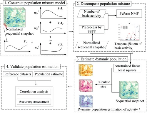
In this study, we present a method of population mixture analysis that uses sequential snapshot data to generate dynamic population distributions by activity type. The method contains four steps: constructing the population mixture model, decomposing the population mixture, estimating the dynamic population distribution, and validating population estimation. This is shown in Figure 1.

Figure 1. The method of population mixture analysis. The NMF refers to the nonnegative matrix factorization algorithm and SSPP refers to the spatial-spectral preprocessing method.

2.1. Construction of the population mixture model

Activities such as working, shopping, and entertainment always occur at regular times (Wu, Cheng, et al. 2020). Existing studies on human mobility also have confirmed that most urban residents’ activities are similar and follow a certain inherent temporal rhythm, making the temporal variations in terms of activity intensity stable (Tu et al. 2017; Liu et al. 2020). We, therefore, assume that the total population’s temporal variation curve of any spatial unit in a region can express as a linear combination of the temporal variation curves i.e. temporal patterns of several basic activities (Equation (1(1) ${\mathrm{P}}_{\mathrm{n}}=\sum _{\mathrm{j}=1}^{\mathrm{J}}{\mathrm{w}}_{\mathrm{n}}^{\mathrm{j}}\mathrm{P}{\mathrm{A}}_{\mathrm{j}}$(1) )). The temporal variation curve means a curve that shows the population size changes over time at a certain time interval. (1) ${\mathrm{P}}_{\mathrm{n}}=\sum _{\mathrm{j}=1}^{\mathrm{J}}{\mathrm{w}}_{\mathrm{n}}^{\mathrm{j}}\mathrm{P}{\mathrm{A}}_{\mathrm{j}}$(1) where ${\mathrm{P}}_{\mathrm{n}}=\left[{\mathrm{P}}_{\mathrm{n}}^1{,\mathrm{P}}_{\mathrm{n}}^2{,\dots ,\mathrm{P}}_{\mathrm{n}}^{\mathrm{t}},\dots ,{\mathrm{P}}_{\mathrm{n}}^{\mathrm{T}}\right]$ is a vector representing the temporal variation curve of the normalized total population in spatial unit n, ${\mathrm{P}}_{\mathrm{n}}^{\mathrm{t}}$ represents the normalized total population in spatial unit n at time t, and T denotes the number of time slots. Parameter J is the number of basic activities in the area, $\mathrm{P}{\mathrm{A}}_{\mathrm{j}}={[\mathrm{P}\mathrm{A}}_{\mathrm{j}}^1{,\mathrm{P}\mathrm{A}}_{\mathrm{j}}^2{,\dots ,\mathrm{P}\mathrm{A}}_{\mathrm{j}}^{\mathrm{t}}{,\dots ,\mathrm{P}\mathrm{A}}_{\mathrm{j}}^{\mathrm{T}}]$ is a vector representing the temporal pattern of activity j, and ${\mathrm{w}}_{\mathrm{n}}^{\mathrm{j}}$ represents the weight of activity j in spatial unit n. The weights in Equation (1(1) ${\mathrm{P}}_{\mathrm{n}}=\sum _{\mathrm{j}=1}^{\mathrm{J}}{\mathrm{w}}_{\mathrm{n}}^{\mathrm{j}}\mathrm{P}{\mathrm{A}}_{\mathrm{j}}$(1) ) need to satisfy both the nonnegative constraint and sum-to-one constraint (Equation (2(2) $\sum _{\mathrm{j}=1}^{\mathrm{J}}{\mathrm{w}}_{\mathrm{n}}^{\mathrm{j}}={1,\mathrm{w}}_{\mathrm{n}}^{\mathrm{j}}\ge 0$(2) )). (2) $\sum _{\mathrm{j}=1}^{\mathrm{J}}{\mathrm{w}}_{\mathrm{n}}^{\mathrm{j}}={1,\mathrm{w}}_{\mathrm{n}}^{\mathrm{j}}\ge 0$(2)

In this process, we derive the original total population’s temporal variation curve for each spatial unit from sequential snapshot data and then normalize it using the sum normalization method to obtain a normalized total population’s curve. Note that the sequential snapshot data are spatially aggregated without personal privacy concerns and the application of the data is not subject to further scrutiny caused by user privacy issues (Chen et al. 2018).

Suppose a sequential snapshot is a time-series image with the size of X×Y×T, where X, Y and T denote rows, columns and the number of times slots, respectively. The product of X and Y, denoted as N, represents that there are total N spatial units. Thus, the population mixture model can be further expressed in the form of matrix multiplication. In other words, the normalized time-series population distribution matrix ${\mathrm{P}}_{\mathrm{N}\times \mathrm{T}}$ can express as a product of the weight matrix ${\mathrm{W}}_{\mathrm{N}\times \mathrm{J}}$ and the temporal pattern matrix of basic activities $\mathrm{P}{\mathrm{A}}_{\mathrm{J}\times \mathrm{T}}$, as shown in Equation (3(3) ${\mathrm{P}}_{\mathrm{N}\times \mathrm{T}}={\mathrm{W}}_{\mathrm{N}\times \mathrm{J}}\mathrm{P}{\mathrm{A}}_{\mathrm{J}\times \mathrm{T}}$(3) ). (3) ${\mathrm{P}}_{\mathrm{N}\times \mathrm{T}}={\mathrm{W}}_{\mathrm{N}\times \mathrm{J}}\mathrm{P}{\mathrm{A}}_{\mathrm{J}\times \mathrm{T}}$(3) where a row vector ${\mathrm{P}}_{\mathrm{n}}$ in matrix ${\mathrm{P}}_{\mathrm{N}\times \mathrm{T}}$ corresponds to the normalized total population variation of unit n, while row vector ${\mathrm{W}}_{\mathrm{n}}$ in matrix ${\mathrm{W}}_{\mathrm{N}\times \mathrm{J}}$ denotes the weights of the J activities in spatial unit n. Matrix $\mathrm{P}{\mathrm{A}}_{\mathrm{J}\times \mathrm{T}}$ is a set of temporal patterns of the basic activities, where the row vector $\mathrm{P}{\mathrm{A}}_{\mathrm{j}}$ corresponds to the temporal pattern of activity j.

2.2. Decomposition of the population mixture

Since it is difficult to directly obtain the temporal pattern of basic activity, it is more appropriate to decompose the above population mixture model using unsupervised methods. The nonnegative matrix factorization (NMF) algorithm factorizes the high-dimensional nonnegative matrix $V_{N\times M}$ into two lower-dimensional nonnegative matrices $W_{N\times D}$ and $H_{D\times M}$ whose product approximates the high-dimensional nonnegative matrix (Eggert and Körner 2004), which can be described by the equation $V_{N\times M}\approx W_{N\times D}{H}_{D\times M}$ and is the same as Equation (3(3) ${\mathrm{P}}_{\mathrm{N}\times \mathrm{T}}={\mathrm{W}}_{\mathrm{N}\times \mathrm{J}}\mathrm{P}{\mathrm{A}}_{\mathrm{J}\times \mathrm{T}}$(3) ). It is, therefore, possible to derive the temporal patterns of several basic activities, i.e. matrix $\mathrm{P}{\mathrm{A}}_{\mathrm{J}\times \mathrm{T}}$ by factorizing matrix ${\mathrm{P}}_{\mathrm{N}\times \mathrm{T}}$ using NMF.

However, NMF tends to fall into a local optimum, making it difficult to obtain a stable optimal solution (Rajabi and Ghassemian 2015). Many scholars have proposed various improved NMF algorithms to solve this problem from the perspective of improving constraints or initialization (Rajabi and Ghassemian 2013; Cao, Zhuo, and Tao 2018). Among these methods, the spatial-spectral preprocessing nonnegative matrix factorization algorithm (SSPP-NMF) can address the NMF’s local minima problem from an initialization perspective, and it has shown promising results in extracting time-series spectral signatures of endmembers (known as pure ground cover materials, e.g. vegetation, impervious surface, and soil) based on temporal mixture analysis in remote sensing science (Guo et al. 2018; Zhuo et al. 2018). Considering the population mixture model is essentially a time-series mixing problem. It is, therefore, suitable for solving the population mixture model with SSPP-NMF. Based on this, we attempt to use the SSPP-NMF algorithm to obtain the temporal pattern of each basic activity. This algorithm first uses SSPP (Martin and Plaza 2012) to preprocess sequential snapshot data to obtain a spatial unit subset, spatially homogeneous areas with one kind of activity, and then uses NMF to decompose the subset to generate temporal patterns of activities. The detailed description is as follows.

1. Preprocessing sequential snapshot using the SSPP method

We preprocess the sequential snapshot using the SSPP method to find a spatial unit subset for matrix factorization. This process contains several steps.

We first process the normalized sequential snapshot with a multiscale Gaussian filtering method and calculate the root mean square error (RMSE) between the processed and original normalized sequential snapshot to measure the spatial homogeneity of each unit. The spatial homogeneity represents the similarity between a unit and its neighbors, and the lower the RMSE, the higher homogeneity of this spatial unit. Then, we use the pixel purity index algorithm (Boardman, Kruse, and Green 1995) to calculate the purity of the unit’s temporal population variation curve to assess the representativeness of each unit. The representativeness measures the possibility that a spatial unit only has one activity, and the higher purity value, the higher representativeness of this spatial unit. Finally, we cluster sequential snapshot using the classical unsupervised classification ISODATA(Iterative Self-Organizing Data Analysis Technique) algorithm (Theodoridis and Koutroumbas 2009) to obtain several clusters, and for each cluster, we select these spatial units with high spatial homogeneity and representativeness as the subset. To derive the subset, rank spatial units according to their homogeneity/representativeness and select the top $\rho /\text{β}$percentage of spatial units as two candidate subsets, whose intersection corresponds to the final subset. In the process, we set $\rho$ = 70 and $\text{β}$ = 30 according to a previous study (Martin and Plaza 2012). At this point, we generate a subset of the sequential snapshot.

(2)	Obtaining the temporal patterns of basic activities

Based on the subset obtained from step (1), we obtain the subset’s time-series population distribution matrix (hereafter called the subset matrix). Suppose the number of basic activities is J. Temporal patterns of J activities can then obtain by decomposing the subset matrix into matrix $\mathrm{P}{\mathrm{A}}_{\mathrm{J}\times \mathrm{T}}$ using NMF. Each row of the matrix represents the temporal pattern of one type of activity.

A critical issue for decomposing the subset matrix using NMF is how to find the optimal parameter J value, as the J value influences the decomposition results. Studies on NMF analysis have attempted to use the index of residual sum of squares (RSS) to optimize this parameter (Hutchins et al. 2008). RSS measures the matrix factorization error between estimated and true values, and a lower value of RSS indicates a more suitable J value. We, therefore, calculate the RSS for different J values (like ranging from 1 to 10) and select the J corresponding to the smallest RSS value as the optimal value.

A detailed description of the RSS calculation. For a given value of parameter J, the NMF factorizes a target matrix ${\mathrm{P}}_{\mathrm{N}\times \mathrm{T}}$ into two matrices ${\mathrm{W}}_{\mathrm{N}\times \mathrm{J}}$ and $\mathrm{P}{\mathrm{A}}_{\mathrm{J}\times \mathrm{T}}$. The estimated target matrix $\widehat{{\mathit{P}}_{N\times T}}$ can then be generated using these two matrices. After that, the RSS(J) between the target matrix ${\mathrm{P}}_{\mathrm{N}\times \mathrm{T}}$ and its estimated matrix $\widehat{{\mathit{P}}_{N\times T}}$ can be computed by Equation (4(4) $RSS\left(J\right)=\sum _{n=1}^N\sum _{t=1}^T(P_{nt}-\widehat{P_{nt}}{)}^2$(4) ). (4) $RSS\left(J\right)=\sum _{n=1}^N\sum _{t=1}^T(P_{nt}-\widehat{P_{nt}}{)}^2$(4) where $P_{nt}$ and $\widehat{P_{nt}}$ are the elements in the n-th row and t-th column of matrix ${\mathrm{P}}_{\mathrm{N}\times \mathrm{T}}$ and matrix $\widehat{P_{N\times T}}$.

(3)	Inferring the specific types of basic activities

Temporal patterns of basic activities can obtain from step (2), however, the specific activity type is unknown. Existing studies have confirmed that citywide human activities have significant temporal rhythms. For example, the number of working activities begins at its lowest in the early morning, reaches its first peak in the morning and its second peak in the afternoon, and declines at night (Tu et al. 2017). Contrary to working activity, in-home activity reaches its maximum at night (Gong et al. 2016). This existing empirical knowledge about various activity temporal rhythms can help us infer the specific activity type. We thus analyse the temporal pattern characteristics and further combine activity temporal rhythm empirical knowledge to infer the specific activity type for each basic activity.

2.3. Estimation of dynamic population distribution by activity type

Determining the activity weights for each unit. After obtaining the activities’ temporal patterns, only the activity weights parameter $W_n$ in Equation (1(1) ${\mathrm{P}}_{\mathrm{n}}=\sum _{\mathrm{j}=1}^{\mathrm{J}}{\mathrm{w}}_{\mathrm{n}}^{\mathrm{j}}\mathrm{P}{\mathrm{A}}_{\mathrm{j}}$(1) ) is unknown. In this situation, the population’s daily variation of a spatial unit n is regarded as a linear function of activity weight, that is, $P_n=W_n\cdot PA$, where $P_n$ and $PA$ are known, and the process of solving $W_n$ can be viewed as a linear least-squares problem that $\underset{W_n}{min}{W}_n\cdot PA-P_n$. We thus use the constrained linear least-squares to solve the activity weight.

With the weights and temporal patterns of basic activities, we can then calculate the dynamic population proportions by activity type. $PopPro{p}_{nj}^t$, the population proportion of activity j in spatial unit n at time t, is calculated by Equation (5(5) ${\mathrm{P}\mathrm{o}\mathrm{p}\mathrm{P}\mathrm{r}\mathrm{o}\mathrm{p}}_{\mathrm{n}\mathrm{j}}^{\mathrm{t}}={\displaystyle \frac{{\mathrm{w}}_{\mathrm{n}}^{\mathrm{j}}{\times \mathrm{P}\mathrm{A}}_{\mathrm{j}}^{\mathrm{t}}}{{\sum }_{\mathrm{j}=1}^{\mathrm{J}}{\mathrm{w}}_{\mathrm{n}}^{\mathrm{j}}{\times \mathrm{P}\mathrm{A}}_{\mathrm{j}}^{\mathrm{t}}}}$(5) ). (5) ${\mathrm{P}\mathrm{o}\mathrm{p}\mathrm{P}\mathrm{r}\mathrm{o}\mathrm{p}}_{\mathrm{n}\mathrm{j}}^{\mathrm{t}}={\displaystyle \frac{{\mathrm{w}}_{\mathrm{n}}^{\mathrm{j}}{\times \mathrm{P}\mathrm{A}}_{\mathrm{j}}^{\mathrm{t}}}{{\sum }_{\mathrm{j}=1}^{\mathrm{J}}{\mathrm{w}}_{\mathrm{n}}^{\mathrm{j}}{\times \mathrm{P}\mathrm{A}}_{\mathrm{j}}^{\mathrm{t}}}}$(5) where ${\mathrm{w}}_{\mathrm{n}}^{\mathrm{j}}$ is the weight of activity j in spatial unit n, and ${\mathrm{P}\mathrm{A}}_{\mathrm{j}}^{\mathrm{t}}$ is the temporal pattern value of activity j at time t.

After obtaining the dynamic population proportions, we further combine it with the original total population in unit n at time t, denoted as $P{o}_n^t$, to calculate the population size engaging in activity j in spatial unit n at time t, labeled as $P_{nj}^t$(Equation (6(6) ${\mathrm{P}}_{\mathrm{n}\mathrm{j}}^{\mathrm{t}}={\mathrm{P}\mathrm{o}\mathrm{p}\mathrm{P}\mathrm{r}\mathrm{o}\mathrm{p}}_{\mathrm{n}\mathrm{j}}^{\mathrm{t}}\times P{o}_n^t$(6) )). (6) ${\mathrm{P}}_{\mathrm{n}\mathrm{j}}^{\mathrm{t}}={\mathrm{P}\mathrm{o}\mathrm{p}\mathrm{P}\mathrm{r}\mathrm{o}\mathrm{p}}_{\mathrm{n}\mathrm{j}}^{\mathrm{t}}\times P{o}_n^t$(6)

After these steps, we finally obtain the dynamic population distributions by activity type and further analyse their corresponding spatiotemporal dynamic patterns.

2.4. Assessment of population estimation results

The lack of real population dynamics for different activity types makes it difficult to comprehensively assess the population estimation results for different activities at different times. Based on the availability of reference data and the connotation of the data, we select employment statistics and WorldPop data for the study area in 2013 as the reference datasets to assess the estimation results at the street scale. The employment data at the street level (level four administrative units) is derived from the 2013 Guangzhou Third National Economic Census, which records the total employed population in each street at the end of 2013 and can be used as a reference to some extent to assess the results of the distribution of the working population. WorldPop is a publicly available gridded population product with a 100-m spatial resolution (https://www.worldpop.org/) and is produced by disaggregating county level (level three administrative unit) census using a random forest algorithm. We use the WorldPop data to some extent to assess the distribution of the stay-at-home population estimated in this study.

We evaluate the population estimation results in two ways. The first way is to perform correlation analysis at the street scale. To do this, we first calculate the averages for each type of population at the street level, and then assess the results by calculating the correlation between the street-level population estimates and the reference datasets. To obtain the reference street-level population from the WorldPop data, we first correct WorldPop's grid values using county-level resident population statistics in 2013 provided by the Guangzhou Statistics Bureau (Equation (7(7) ${\mathrm{W}\mathrm{o}\mathrm{r}\mathrm{l}\mathrm{d}\mathrm{P}\mathrm{o}\mathrm{p}}_{\mathrm{i}}^{\mathrm{m}}=WorldPo{p}_i\times {\displaystyle \frac{ResidentPo{p}_k}{{\sum }_{i\in k}WorldPo{p}_i}}$(7) )) and then aggregate the grids to street units. (7) ${\mathrm{W}\mathrm{o}\mathrm{r}\mathrm{l}\mathrm{d}\mathrm{P}\mathrm{o}\mathrm{p}}_{\mathrm{i}}^{\mathrm{m}}=WorldPo{p}_i\times {\displaystyle \frac{ResidentPo{p}_k}{{\sum }_{i\in k}WorldPo{p}_i}}$(7) where $WorldPo{p}_i^m$ is the modified population count of grid i, $WorldPo{p}_i$ is the raw population count, and $ResidentPo{p}_k$ is the resident population count of county k.

In addition, we further quantify the accuracy of the population estimate results using the work-to-household ratio, defined as the ratio of the working population to the total residents on each street. To do this, we first calculate the reference work-to-household ratio value for each street via dividing the total employed population from employment data by the population obtained from WorldPop data. The estimated work-to-household ratio is also calculated based on population estimation results. Then, we quantitatively assess the estimation error by calculating the mean absolute error (MAE) and RMSE based on the estimated and reference ratio values, respectively. We also assess the degree of fitting by plotting a scatterplot of the reference and estimated ratio values and calculating the coefficient of determination (R²).

3. Case study and data description

We apply the population mixture analysis method to the RTUD data in Guangzhou for empirical analysis.

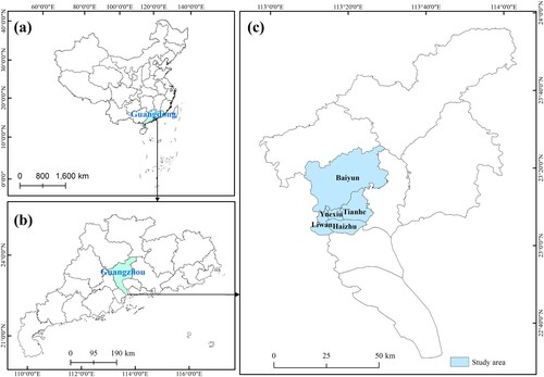
Five central urban districts (Haizhu, Yuexiu, Liwan, Tianhe, and Baiyun) of Guangzhou city in Guangdong Province, China are selected as the study area (Figure 2). According to the Guangzhou statistical yearbook in 2016 (https://lwzb.gzstats.gov.cn:20001/datav/admin/home/www_nj/), the total area of the study area is 1,075.42 km², which is approximately 14.47% of the total area of Guangzhou. The registered resident population in 2015 reached 7,641,300, accounting for 56.6% of the total resident population in Guangzhou. The five central districts occupy the top five highest population densities among all the districts in Guangzhou. As the political, economic and cultural center of Guangzhou, study area has experienced continued population growth in recent years, which has brought serious challenges to the allocation of medical facilities, housing, transportation, education and other resources.

Figure 2. The geographical location of our study area. (a) the study area in China; (b) the study area in Guangdong Province; (c) the spatial distribution of the five central urban districts of Guangzhou including Haizhu, Yuexiu, Liwan, Tianhe, and Baiyun.

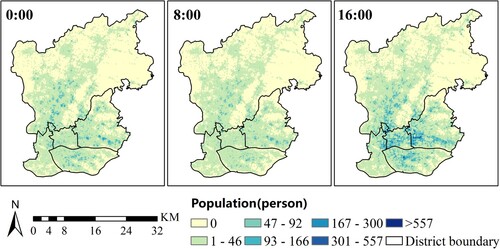
The RTUD data, a kind of sequential snapshot data, are used to estimate the hourly population proportion and population size by activity type. When mobile phone users use Tencent’s location service products such as the instant message applications of QQ and WeChat or the navigation application Tencent Maps, their locations are recorded, which enables the RTUD to store an hourly number of active smartphone users at a spatial resolution of 25 meters. According to Tencent's WeChat data report, China’s monthly active WeChat users reached 549 million in 2015. Meanwhile, Tencent's survey results show that the WeChat penetration rate has exceeded 93% in 2015 in China’s first-tier cities such as Beijing, Shanghai, Guangzhou and Shenzhen. Due to its huge user base, RTUD can serve as a representative indicator of the real-time population dynamic distribution. In this case study, we apply a web crawler to collect RTUD data from June 15 to June 19, 2015, which is five consecutive working days from Monday to Friday. Note that the data are spatially aggregated without personal privacy concerns. To derive the hourly population distribution on weekdays, we first average the five consecutive working days and then aggregate them into 100-m grids. After a series of preprocessing steps, including coordinate correction, grid statistics and vector rasterization, we generate a time-series RTUD image with 24 bands, with each band representing the population distribution at a specific hour. Taking 0:00, 8:00 and 16:00 as examples, Figure 3 illustrates the population distribution at different times of the day. Complete 24 h RTUD images are shown in the Appendix (see Figure A1).

Figure 3. Averaged RTUD images at different times of weekdays in the study area.

4. Results and analysis

4.1. Temporal patterns of basic activities in study area

Following the steps described in Section 2.2, we perform unsupervised NMF decomposition with different J values (ranging from 1 to 10) and evaluate the results based on the RSS index. Figure 4(a) shows that the RSS value decreases significantly when the value of J increases, while the lowest RSS value appears when J is set to 3. When J increases from 4 to 8, the RSS value begins to fluctuate with a local minimum appearing at the value of 5. Since the existing study suggests choosing the first value where the RSS curve presents a significant inflection point (Hutchins et al. 2008), we set the number of basic activities in our study area as 3 in the subsequent analyses. Figure 4(b) shows the temporal patterns of the three activities.

Figure 4. (a) Variation of RSS value with the number of basic activities. (b) Temporal patterns of three basic activities.

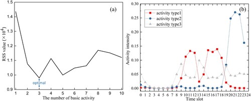
We further combine the temporal pattern characteristics to infer the specific activity type for each basic activity. Type 1 has two stable activity intensity peaks, one in the morning and the other in the afternoon, which are consistent with the working hours. In addition, its activity intensity during the daytime is higher than that at nighttime. Therefore, we define type 1 as working activity. The activity intensity of type 2 is relatively stable during the daytime but increases significantly during the nighttime. These characteristics are similar to home activities, therefore, we identify type 2 as stay-at-home activity. Type 3 has three short-term activity intensity peaks in the morning, noon, and afternoon, with the peak at noon being the highest. In addition, the activity intensities of type 3 during the nighttime are between those of type 1 and type 2 and tend to be stable, which makes it more likely to represent other daily activities excluding work and home activities such as transportation, shopping, and entertainment. We hence define activity 3 as social activity.

The curve shapes of type 1 and type 2 are similar to the characteristic curve of people at work and at home over time obtained by Järv, Tenkanen, and Toivonen (2017). The curve shape of type 3 is consistent with hourly changes in the social activity counts extracted by Tu et al. (2017) using mobile phone data. These similarities demonstrate that the activity types and their activity intensity curves obtained using the method of this paper are reasonable and credible.

The population groups corresponding to the three activities are, therefore, named the working population, stay-at-home population, and socializing population respectively in the subsequent results.

4.2. Assessment for decomposing results of mixed population

As each activity pattern tends to be stable in the 10:00-12:00, 15:00-17:00 and 20:00-22:00 periods and the first two periods are close (Figure 4(b)), we define 10:00-12:00 and 15:00-17:00 periods as working hours and 20:00-22:00 period as at-home hours. Then, we calculate averages of population estimation for three activities at the street level during working hours and at-home hours respectively. Taking the average working population estimation at the street level during working hours as an example, we first aggregate the spatial units within the street to obtain the street scale hourly working population estimation and then calculate its average during working hours. Finally, calculate the Spearman rank correlation coefficients for the three scenarios, including the correlations between the street-level estimated population of three activities during working hours and employment data, between the street-level estimated population of three activities during at-home hours and WorldPop, and between raw RTUD during working hours/ at-home hours and employment data/ WorldPop.

The Spearman correlation coefficient for each period in Table 1 has passed the significance test with a confidence level of P value less than 0.05. Compared with the population of other activities, the estimated stay-at-home home population during at-home hours exhibits the highest and most positive correlation coefficient with the WorldPop, reaching 0.707. Meanwhile, the estimated working population during working hours has the most significant positive correlation with employment data, with the largest correlation coefficient of 0.747. These results indicate the reliability of the population estimation results. In addition, both the raw RTUD during working hours and at-home hours have lower correlations with employment and WorldPop, suggesting that it is inappropriate to directly use time-specific RTUD values as a proxy for the population engaging in a specific activity. Instead, decomposing the population from sequential snapshot data proves to be a suitable means to obtain the population by activity type.

Table 1. Results for Spearman rank correlation analysis.

Reference datasets	Estimated population by activity type during different periods
employment	Working hours
	Working population	Stay-at-home population	Socializing population	Raw RTUD
	0.747	0.423	0.558	0.670
WorldPop	At-home hours
	Working population	Stay-at-home population	Socializing population	Raw RTUD
	0.539	0.707	0.602	0.614

Furthermore, we calculate the two estimated work-to-household ratios: the ratio based on population decomposition and the ratio based on raw RTUD. The former is calculated by dividing the street-level working population estimation during working hours by the stay-at-home population estimation during at-home hours. The latter is generated by dividing the street-level RTUD during working hours by that during at-home hours.

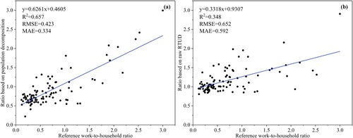
Figure 5 shows the estimation error distribution for each street. The estimation error based on population decomposition is smaller than that based on raw RTUD. The former is mainly concentrated in the range of −0.5–0.5, while the latter is mainly concentrated in the interval of −1–0.5. Moreover, compared to the ratio based on the raw RTUD, the ratio based on population decomposition displays superior performance in terms of the three evaluation metrics. Figure 6 shows that the ratio based on population decomposition is more closely related to the reference ratio, with a higher R² value (0.657 vs. 0.348) and lower RMSE and MAE values (0.423/0.334 vs. 0.652/0.592). These evaluation results again reveal the reliability of the population estimation results and the necessity of population decomposition.

Figure 5. Work-to-household ratio estimation error distribution for each street. (a) Estimation error based on population decomposition, and (b) estimation error based on raw RTUD.

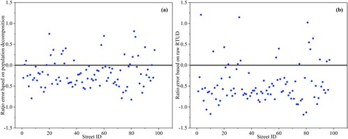
Figure 6. Scatterplots of reference work-to-household ratio and estimated work-to-household ratio based on (a) population decomposition and (b) raw RTUD.

4.3. Exploring population dynamic distribution characteristics for different activities

4.3.1. Temporal changes of population density at the district level

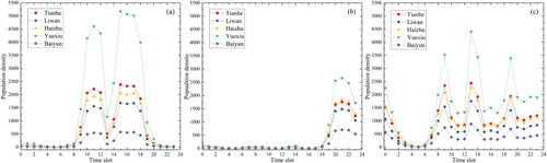
Overall, the fluctuations in population density within a day for different human activities show similar trends in all five central districts of Guangzhou (Figure 7). Among the five districts, Yuexiu district has the highest population density for all three human activities, followed by Tianhe district and Haizhu district, whose population density values are very close to each other. These results reflect the fact that Yuexiu district is the oldest central area as well as the administrative, commercial, financial and cultural center. Although Tianhe district has the Guangzhou central business district (CBD), one of the three CBDs in China, and is considered as the new city center of Guangzhou, its population density is still lower than that of Yuexiu district. In contrast, Baiyun district has the sparsest population density in all activities due to its large area and small population size.

Figure 7. Temporal changes in population densities for different human activities in central districts of Guangzhou. (a) Working population, (b) Stay-at-home population and (c) Socializing population.

4.3.2. Spatial dynamic patterns of population by activity type

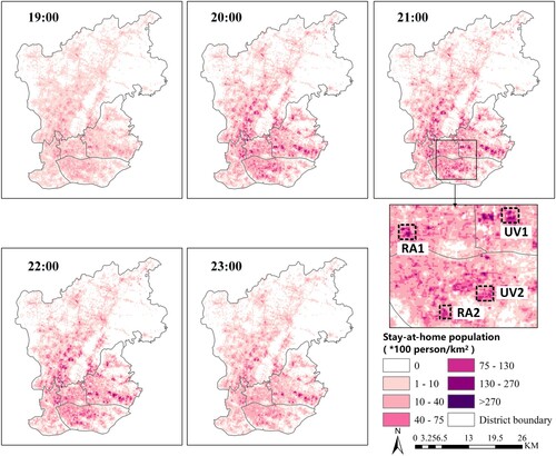
Since the population distribution at the adjacent time is similar, we select six hours with significant intensity differences for each activity (9:00, 11:00, 13:00, 15:00, 19:00, and 21:00) to analyse the dynamic spatial distribution patterns of the working and socializing population. Since the stay-at-home population is small in number and changes little during the daytime, we only analyse its hourly distribution pattern in the period of 19:00-23:00. Based on these results, we summarize the spatial dynamic patterns for the three population groups in this study area.

1. The dynamic distribution of the working population reproduces the regular work scenarios. At the peak working hours (11:00 and 15:00), both the density and spatial extent of the working population are significantly greater than other hours. There are obvious hotspots for the working population, which mainly concentrate in regions with multiple office buildings and commercial service centers, such as the office buildings located around the commercial centers of Tianhe Sports Center and Zhujiang New Town and (regions OB1 and OB2 in Figure 8), the clothing market and trade city in Yuexiu district (region CS1 in Figure 8), and the international textile city in Haizhu district (region CS2 in Figure 8). At noon, the spatially aggregated hotspots shift to some commercial service places (regions CS3-CS5 in Figure 8), which is consistent with the fact that people with different jobs have different working time characteristics. During other non-working hours, the spatial aggregation of the working population gradually disappears and shows a scattered distribution pattern. It can be observed that the population size in the office buildings changes the most drastically, which is in line with the actual situation.

2. The socializing population presents more complex spatial patterns. Different spatial aggregation patterns can find at 9:00, 13:00 and 19:00, while a scattered pattern can observe at other hours (Figure 9). At 9:00, a majority of the socializing population aggregates in the transportation hubs, including subway stations, bus stations and coach terminal stations (regions SS, BS and CTS in Figure 9), while a few distribute in urban villages (regions UV in Figure 9) or around hospital (region Hosp in Figure 9). At 13:00, the socializing population increases and shows an obvious spatial aggregation pattern in some large commercial and entertainment centers (regions CE in Figure 9), which coincides with people’s dining and shopping activities. At 19:00, the socializing population gathers again at the transportation hubs and the surrounding shopping malls such as the Tianhecheng department store around the Tiyuxi subway station, and Liying plaza around the Kecun subway station.

3. The stay-at-home population gradually increases from 19:00–22:00 and decreases slightly at 23:00. In terms of the spatial distribution pattern, the population is dispersed at 19:00 and gradually shifts to an agglomeration pattern. The main agglomeration centers are located in residential areas (regions RA in Figure 10) and urban villages (regions UV in Figure 10).

Figure 8. Dynamic spatial distributions of working population in the study area. ‘OB’ refers to official building, and regions OB1and OB2 are the office buildings around Tianhe Sports Center and Zhujiang New Town; ‘CS’ refers to commercial services, and regions CS1to CS5 correspond to Clothing market and trade city, International textile city, Clothing market, Mopark department store and Tianyu plaza, and International textile city.

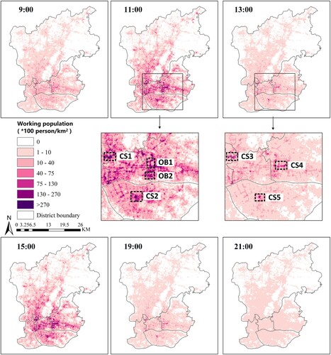
Figure 9. Spatial distributions of socializing population at different hours in the study area. ‘CTS’ refers to coach terminal station, and region CTS is Guangdong coach terminal station and Guangzhou railway station; ‘Hosp’ refers to the hospital, and region Hosp is Zhongshan ophthalmic center and Guangzhou women and children medical center; ‘SS’ refers to the subway stations, and regions SS1 and SS2 and the Ganging subway station and Kecun subway station; ‘BS’ refers to bus station, and region BS is Chebei bus station; ‘UV’ refers to urban villages, and areas UV1 to UV2 correspond to Kangle village and Shangyong village. ‘CE’ refers to the commercial and entertainment centers, and areas CE1 and CE2 are the Beijing road commercial pedestrian street and shopping malls of TaiKoo hui and Teemall.

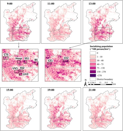
Figure 10. Dynamic distributions of the stay-at-home population in the study area. ‘RA’ refers to the residential areas, and regions RA1 and RA2 correspond to Caiyuan community and Jiayi garden; ‘UV’ refers to the urban village, and regions UV1 and UV2 are Tangdang village and Shangyong village.

5. Discussion

5.1. Potential relationship between dynamic population proportions and regional functions

What determines the population proportions of the three activities and their changing characteristics during the day, and are these related to functional areas? From the dynamic population proportions, it is easy to find that the dominant population varies at different periods in the study area. During the daytime, working and socializing are the main components of the urban population, accounting for 97.44%, while the working population accounts for 61% during working hours. At nighttime (20:00-23:00), more than half of the population (57%) stays at home. In general, urban areas with diverse functions serve a variety of human activities throughout the day, making the urban function vary at different times of the day, such as a working function during the daytime and a residential function at night, which is consistent with the dominant population.

To further explore the association between the population proportions of the three activities and diverse regional functions, we take three sample areas as examples for detailed analyses. Figure 11 shows the satellite images of the three sample regions (Figure 11(a1), (b1) and (c1)) as well as their hourly populations of three activities (Figure 11(a2), (b2) and (c2)).

Figure 11. Satellite images of the three sample regions. (a1) Nanzhou garden with residential and commercial functions; (b1) Liying plaza with commerce, transportation, work and residence functions; (c1) the People's Municipal Government of Guangzhou with work function, and (a2-c2) are the hourly population of regions a1 to c1.

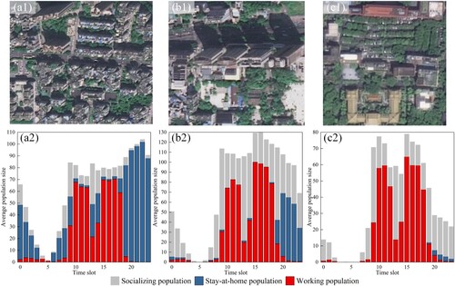
Sample area 1 is Nanzhou Garden, a residential community in Haizhu district (Figure 11(a1)), where most buildings’ ground floors are used for commercial purposes. The composition of this area’s population shows a pattern of the predominant working population during the daytime and stay-at-home population at nighttime (Figure 11(a2)), which is consistent with its mixed commercial and residential functions.

Sample area 2 is Liying Plaza in Haizhu District, adjacent to the Kecun subway station (Figure 11(b1)). This area has a complex composition of shopping malls, offices, and residences. The human activity in this area also shows characteristics consistent with its functions (Figure 11(b2)). The population participating in social activity occupies a certain proportion every hour throughout the day and peaks at 9:00 am and 1:00 pm, which is consistent with its functions as both a transportation hub and commercial attraction. The size of working population is the largest during working hours due to the existence of multiple office buildings in the area. The stay-at-home population becomes the main part during the night hours, which corresponds to the area’s residential function.

Buildings in sample area 3 are mostly office buildings of the People's Municipal Government of Guangzhou (Figure 11(c1)). The human activities in this area show a relatively obvious working pattern (Figure 11(c2)). The working population accounts for the vast majority of the total population during working hours, followed by the socializing population and a very small proportion of the home-based population. Similar to the other two areas, the predominant working population of this area is consistent with its working function.

The above analyses of the three sample areas provide good evidence again that there is an intrinsic correlation between a region's diverse functions and its characteristics of dynamic population structure in terms of activity types. This finding may provide urban planning departments with some insights into how to design a region’s functions more rationally to obtain the required crowd dynamics. However, more effort is needed to quantify the relationship in depth.

5.2. Comparison with previous studies

In this study, we present a method of population mixture analysis to mine the dynamic population distributions by activity type based on decomposing sequential snapshot data. Compared with previous studies, this method has three advantages. First, unlike most studies on mapping population dynamics (Silva et al. 2020; Cheng, Wang, and Ge 2022; Zhao et al. 2021), our research can enrich the activity semantics for dynamic population distribution. Second, both the sequential snapshot data and the population mixture used in the method are novel. From the data source aspect, the sequential snapshot data has been spatially aggregated to represent aggregated level population distribution, making it more readily available, while previous studies required massive individual-level human mobility data (e.g. mobile phone data) (Wu, Cheng, et al. 2020; Liu et al. 2021), which may pose individual security and privacy threats and are usually inaccessible to common people. To preserve the privacy of individual trajectory data, scholars have proposed many trajectory privacy protection methods (Jin et al. 2022; Talat et al. 2020). Moreover, apart from RTUD, there are other available sequential snapshot data to support this research. The sequential snapshot data of population distribution can be generated from location service applications in mobile phones or other mobile phone data. It is, therefore, very possible to obtain similar aggregated mobile phone data from telecommunication operators or mobile phone applications, such as Facebook, Twitter, or GoogleMap. From the methodology aspect, existing studies (Çolak et al. 2015; Yin, Lin, and Zhao 2021) needed to combine various complex methods (e.g. hidden Markov model) with additional auxiliary data (e.g. travel surveys, POI and land use information) that could provide a priori knowledge related to activities. In contrast, the method of decomposing population mixture (NMF-based method used in our study) belongs to data-driven and it does not require other auxiliary data which makes it much easier to implement. Third, the substitutability of sequential snapshot data and independence from prior knowledge benefit the proposed method with great potential for application in other regions. Consequently, our method can, therefore, serve as a simple but effective solution to capture the hourly population dynamics by activity type.

Although both correlation analysis and accuracy assessment for population estimation results prove that decomposing population mixture is reasonable, there are still several limitations and uncertainties. First, similar to previous studies based on individual-level mobile phone data (Liu et al. 2021; Qian et al. 2021), there is no guarantee that all mobile phone users are active at every moment, and RTUD data still cannot cover all age groups of the population, especially children and elderly people who do not use mobile phones. Thus, the RTUD data are regarded as a type of biased sampling of the entire population, and the estimated hourly population distribution based on RTUD is also skewed and cannot represent the entire population. Second, for basic activity, the obtained three activities are a coarse representation of residents’ daily activities, and the activity type is inferred by combing empirical knowledge about activity temporal rhythms. Although more activities can discover as long as setting the parameter J greater than 3, many activity types are hardly inferred and associated with specific population groups due to insufficient study of activity behavior patterns and lack of activity temporal rhythms knowledge. Additionally, there can be uncertainties in evaluating population estimation results when only assessing the quality of dynamic population estimates at the street level for a given period. It is challenging to verify the estimated population on finer spatial and temporal scales unless appropriate validation data are available. In addition, we assume that the temporal pattern of each basic activity is stable within a certain region and neglect its spatial heterogeneity, especially in regions with different socioeconomic statuses. The normalization method used in our study could reduce the heterogeneity to a certain extent and better solutions can make further explored in subsequent studies.

6. Conclusion

This study presents a method for mining the dynamic population distributions by activity type based on the decomposition of sequential snapshot data. There are three primary steps of the method: constructing a population mixture model using sequential snapshot data, decomposing the population mixture, and estimating the dynamic population size for each activity. After obtaining the dynamic population distributions for each activity, we further analyse their spatiotemporal dynamics. We use real-time Tencent user density data of five central districts in Guangzhou city as an example to illustrate the process and validate the reliability of population estimation.

In the population mixture analysis, we extract the dynamic population with three typical activity types per hour in the central districts of Guangzhou. The population estimation results show good correlations with the reference population from employment statistics and WorldPop data. The estimated stay-at-home population during at-home hours has the highest Spearman rank correlation coefficients with WorldPop, reaching 0.707, and the working population during working hours has the highest correlation coefficient value of 0.747 with employment. Moreover, the population decomposition result has superior performance in calculating the work-to-household ratio, with a higher R² value of 0.657 and lower RMSE and MAE values. These analyses reveal the reliability of the population estimation results.

Analyses of the spatial dynamic patterns show that the population by activity type in the central districts of Guangzhou have significant differences in their temporal distributions. The working population mainly concentrates in office buildings and commercial centers and displays aggregated hotspots during working hours, and a scattered distribution can be observed during non-working hours. On the contrary, the socializing population shows scattered patterns during working hours, and spatial aggregation patterns during non-working hours can find in transportation hubs and commercial and entertainment centers. In addition, from the estimated hourly population, we find an underlying relationship between a region’s diverse functions and its dynamic population structure in terms of activity type. This finding may provide new insight for scholars to study urban dynamic functions and for planning departments to design regional functions more rationally.

Geolocation information

The study area in this paper is the central districts of Guangzhou city, China, which include Haizhu district, Yuexiu district, Liwan district, Tianhe district, and Baiyun district.

Data availability statement

We provided sample data and codes to make our research reproducible, accessed in GitHub (https://github.com/shiql/PopulationMixture).

Disclosure statement

No potential conflict of interest was reported by the author(s).

Additional information

Funding

This research was funded by the National Natural Science Foundation of China [grant numbers 41971372 and 41971345], the Natural Science Foundation of Guangdong Province [grant number 2020A1515010680], and the Innovation Group Project of Southern Marine Science and Engineering Guangdong Laboratory (Zhuhai) [grant number 311021004.

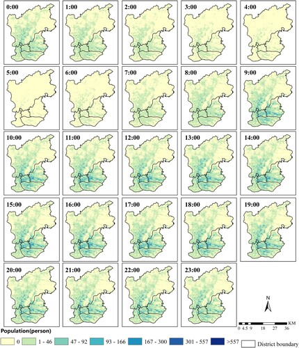
Appendix

Figure A1. Averaged 24 h RTUD images of weekdays in the study area.

References

- Bhaduri, Budhendra, Edward Bright, Phillip Coleman, and Marie L. Urban. 2007. “LandScan USA: A High-Resolution Geospatial and Temporal Modeling Approach for Population Distribution and Dynamics.” GeoJournal 69 (1): 103–117. doi:10.1007/s10708-007-9105-9.
- Boardman, Joseph W., Fred A. Kruse, and Robert O. Green. 1995. “Mapping Target Signatures via Partial Unmixing of Aviris Data.” Paper presented at the summaries of the fifth annual JPL airborne Earth Science workshop, pasadena, January 23-26.
- Cao, Jingjing, Li Zhuo, and Haiyan Tao. 2018. “An Endmember Initialization Scheme for Nonnegative Matrix Factorization and Its Application in Hyperspectral Unmixing.” ISPRS International Journal of Geo-Information 7 (5): 195. doi:10.3390/ijgi7050195.
- Chen, Yiyong, Xiaoping Liu, Wenxiu Gao, Raymond Yu Wang, Yun Li, and Wei Tu. 2018. “Emerging Social Media Data on Measuring Urban Park Use.” Urban Forestry & Urban Greening 31: 130–141. doi:10.1016/j.ufug.2018.02.005.
- Cheng, Zhifeng, Jianghao Wang, and Yong Ge. 2022. “Mapping Monthly Population Distribution and Variation at 1-km Resolution Across China.” International Journal of Geographical Information Science, 1166–1184. doi:10.1080/13658816.2020.1854767.
- Çolak, Serdar, Lauren P. Alexander, Bernardo G. Alvim, Shomik R. Mehndiratta, and Marta C. González. 2015. “Analyzing Cell Phone Location Data for Urban Travel.” Transportation Research Record: Journal of the Transportation Research Board 2526 (1): 126–135. doi:10.3141/2526-14.
- Deng, Chengbin, and Changshan Wu. 2013. “A Spatially Adaptive Spectral Mixture Analysis for Mapping Subpixel Urban Impervious Surface Distribution.” Remote Sensing of Environment 133: 62–70. doi:10.1016/j.rse.2013.02.005.
- Diao, Mi, Yi Zhu, Joseph Ferreira, and Carlo Ratti. 2016. “Inferring Individual Daily Activities from Mobile Phone Traces: A Boston Example.” Environment and Planning B: Planning and Design 43 (5): 920–940. doi:10.1177/0265813515600896.
- Eggert, Julian, and Edgar Körner. 2004. “Sparse Coding and NMF.” Paper presented at the IEEE International joint Conference on neural Networks (IEEE Cat. No.04CH37541), 25-29 July 2004.
- Gong, Li, Xi Liu, Lun Wu, and Yu Liu. 2016. “Inferring Trip Purposes and Uncovering Travel Patterns from Taxi Trajectory Data.” Cartography and Geographic Information Science 43 (2): 103–114. doi:10.1080/15230406.2015.1014424.
- Greger, Konstantin. 2015. “Spatio-Temporal Building Population Estimation for Highly Urbanized Areas Using GIS.” Transactions in GIS 19 (1): 129–150. doi:10.1111/tgis.12086.
- Guo, Yubo, Li Zhuo, Haiyan Tao, Jingjing Cao, and Fang Wang. 2018. “Spatial-Spectral Preprocessing Based on Nonnegative Matrix Factorization to Unmix Hyperspectral Data.” Remote Sensing Technology and Application 33 (2): 216–226.
- Hanaoka, Kazumasa. 2018. “New Insights on Relationships Between Street Crimes and Ambient Population: Use of Hourly Population Data Estimated from Mobile Phone Users’ Locations.” Environment and Planning B: Urban Analytics and City Science 45 (2): 295–311. doi:10.1177/0265813516672454.
- Huang, Xiao, Cuizhen Wang, Zhenlong Li, and Huan Ning. 2021. “A 100 m Population Grid in the CONUS by Disaggregating Census Data with Open-Source Microsoft Building Footprints.” Big Earth Data 5 (1): 112–133. doi:10.1080/20964471.2020.1776200.
- Hutchins, Lucie N., Sean M. Murphy, Priyam Singh, and Joel H. Graber. 2008. “Position-Dependent Motif Characterization Using Non-Negative Matrix Factorization.” Bioinformatics (oxford, England) 24 (23): 2684–2690. doi:10.1093/bioinformatics/btn526.
- Järv, Olle, Henrikki Tenkanen, and Tuuli Toivonen. 2017. “Enhancing Spatial Accuracy of Mobile Phone Data Using Multi-Temporal Dasymetric Interpolation.” International Journal of Geographical Information Science 31 (8): 1630–1651. doi:10.1080/13658816.2017.1287369.
- Jin, Fengmei, Wen Hua, Matteo Francia, Pingfu Chao, Maria Orowska, and Xiaofang Zhou. 2022. “A Survey and Experimental Study on Privacy-Preserving Trajectory Data Publishing.” IEEE Transactions on Knowledge and Data Engineering, doi:10.1109/TKDE.2022.3174204.
- Kang, Chaogui, Li Shi, Fahui Wang, and Yu Liu. 2020. “How Urban Places are Visited by Social Groups? Evidence from Matrix Factorization on Mobile Phone Data.” Transactions in GIS 24 (6): 1504–1525. doi:10.1111/tgis.12654.
- Liu, Shaojun, Yi Long, Ling Zhang, and Hao Liu. 2021. “Semantic Enhancement of Human Urban Activity Chain Construction Using Mobile Phone Signaling Data.” ISPRS International Journal of Geo-Information 10 (8): 545. doi:10.3390/ijgi10080545.
- Liu, Huimin, Yiyuan Xu, Jianbo Tang, Min Deng, Jincai Huang, Wentao Yang, and Fang Wu. 2020. “Recognizing Urban Functional Zones by a Hierarchical Fusion Method Considering Landscape Features and Human Activities.” Transactions in GIS 24 (5): 1359–1381. doi:10.1111/tgis.12642.
- Martin, Gabriel, and Antonio Plaza. 2012. “Spatial-Spectral Preprocessing Prior to Endmember Identification and Unmixing of Remotely Sensed Hyperspectral Data.” IEEE Journal of Selected Topics in Applied Earth Observations and Remote Sensing 5 (2): 380–395. doi:10.1109/JSTARS.2012.2192472.
- Mistry, D., Litvinova, M., Pastore y Piontti, A., Chinazzi, M., Fumanelli, L., Gomes, M.F., Haque, S.A., Liu, Q.H., Mu, K., Xiong, X. and Halloran, M.E. 2021. “Inferring High-Resolution Human Mixing Patterns for Disease Modeling.” Nature Communications 12 (1):323. doi:10.1038/s41467-020-20544-y.
- Park, Jaehee, Hao Zhang, Su Yeon Han, Atsushi Nara, and Ming-Hsiang Tsou. 2020. “Estimating Hourly Population Distribution Patterns at High Spatiotemporal Resolution in Urban Areas Using Geo-Tagged Tweets and Dasymetric Mapping.” Paper presented at the 11th International Conference on Geographic Information Science (GIScience 2021)-part I.
- Qian, Chen, Weifeng Li, Zhengyu Duan, Dongyuan Yang, and Bin Ran. 2021. “Using Mobile Phone Data to Determine Spatial Correlations Between Tourism Facilities.” Journal of Transport Geography 92 (92): 103018. doi:10.1016/j.jtrangeo.2021.103018.
- Rajabi, Roozbeh, and Hassan Ghassemian. 2013. “Hyperspectral Data Unmixing Using GNMF Method and Sparseness Constraint.” Paper presented at the IEEE International Geoscience and Remote Sensing symposium - IGARSS, 21-26 July 2013.
- Rajabi, Roozbeh, and Hassan Ghassemian. 2015. “Spectral Unmixing of Hyperspectral Imagery Using Multilayer NMF.” IEEE Geoscience and Remote Sensing Letters 12 (1): 38–42. doi:10.1109/LGRS.2014.2325874.
- Shang, Shuoshuo, Shihong Du, Shouji Du, and Shoujie Zhu. 2021. “Estimating Building-Scale Population Using Multi-Source Spatial Data.” Cities 111, doi:10.1016/j.cities.2020.103002.
- Silva, Batista e, Sérgio Freire Filipe, Marcello Schiavina, Konštantín Rosina, Mario Alberto Marín-Herrera, Lukasz Ziemba, Massimo Craglia, Eric Koomen, and Carlo Lavalle. 2020. “Uncovering Temporal Changes in Europe’s Population Density Patterns Using a Data Fusion Approach.” Nature Communications 11 (1): 1–11. doi:10.1038/s41467-020-18344-5.
- Song, Y., B. Chen, H. C. Ho, M. P. Kwan, D. Liu, F. Wang, J. Wang, et al. 2021. “Observed Inequality in Urban Greenspace Exposure in China.” Environment International 156: 106778. doi:10.1016/j.envint.2021.106778.
- Song, Yimeng, Bo Huang, Jixuan Cai, and Bin Chen. 2018. “Dynamic Assessments of Population Exposure to Urban Greenspace Using Multi-Source Big Data.” Science of the Total Environment 634: 1315–1325. doi:10.1016/j.scitotenv.2018.04.061.
- Song, Yimeng, Bo Huang, Qingqing He, Bin Chen, Jing Wei, and Rashed Mahmood. 2019. “Dynamic Assessment of PM2.5 Exposure and Health Risk Using Remote Sensing and Geo-Spatial Big Data.” Environmental Pollution 253: 288–296. doi:10.1016/j.envpol.2019.06.057.
- Stevens, Forrest R., Andrea E. Gaughan, Catherine Linard, and Andrew J. Tatem. 2015. “Disaggregating Census Data for Population Mapping Using Random Forests with Remotely-Sensed and Ancillary Data.” PLoS ONE 10 (2): e0107042. doi:10.1371/journal.pone.0107042.
- Talat, Romana, Mohammad S. Obaidat, Muhammad Muzammal, Ali Hassan Sodhro, Zongwei Luo, and Sandeep Pirbhulal. 2020. “A Decentralised Approach to Privacy Preserving Trajectory Mining.” Future Generation Computer Systems 102: 382–392. doi:10.1016/j.future.2019.07.068.
- Tatem, Andrew J., Susana Adamo, Nita Bharti, Clara R. Burgert, Marcia Castro, Audrey Dorelien, Gunter Fink, et al. 2012. “Mapping Populations at Risk: Improving Spatial Demographic Data for Infectious Disease Modeling and Metric Derivation.” Population Health Metrics 10 (1): 8. doi:10.1186/1478-7954-10-8.
- Theodoridis, Sergios, and Konstantinos Koutroumbas. 2009. Pattern Recognition (Fourth Edition). Boston: Academic Press.
- Tu, Wei, Jinzhou Cao, Yang Yue, Shih-Lung Shaw, Meng Zhou, Zhensheng Wang, Xiaomeng Chang, Yang Xu, and Qingquan Li. 2017. “Coupling Mobile Phone and Social Media Data: A New Approach to Understanding Urban Functions and Diurnal Patterns.” International Journal of Geographical Information Science 31 (12): 2331–2358. doi:10.1080/13658816.2017.1356464.
- Wu, Lun, Ximeng Cheng, Chaogui Kang, Di Zhu, Zhou Huang, and Yu Liu. 2020. “A Framework for Mixed-Use Decomposition Based on Temporal Activity Signatures Extracted from Big Geo-Data.” International Journal of Digital Earth 13 (6): 708–726. doi:10.1080/17538947.2018.1556353.
- Wu, Yimin, Liang Wang, Linghui Fan, Ming Yang, Yu Zhang, and Yongheng Feng. 2020. “Comparison of the Spatiotemporal Mobility Patterns Among Typical Subgroups of the Actual Population with Mobile Phone Data: A Case Study of Beijing.” Cities 100 (1): 102670. doi:10.1016/j.cities.2020.102670.
- Xing, Xiaoyue, Zhou Huang, Di Zhu Ximeng Cheng, Chaogui Kang, Fan Zhang, and Yu Liu. 2020. “Mapping Human Activity Volumes Through Remote Sensing Imagery.” IEEE Journal of Selected Topics in Applied Earth Observations and Remote Sensing 13: 5652–5668. doi:10.1109/JSTARS.2020.3023730.
- Xu, Yang, Shih-Lung Shaw, Feng Lu, Jie Chen, and Qingquan Li. 2018. “Uncovering the Relationships Between Phone Communication Activities and Spatiotemporal Distribution of Mobile Phone Users.” In Human Dynamics Research in Smart and Connected Communities, edited by Shih-Lung Shaw, and Daniel Sui, 41–65. Cham: Springer International Publishing.
- Yang, Bo, Xiao Fu, Nicholas D. Sidiropoulos, and Kejun Huang. 2020. “Learning Nonlinear Mixtures: Identifiability and Algorithm.” IEEE Transactions on Signal Processing 68: 2857–2869. doi:10.1109/TSP.2020.2989551.
- Yang, Jing, Disheng Yi, Bowen Qiao, and Jing Zhang. 2019. “Spatio-Temporal Change Characteristics of Spatial-Interaction Networks: Case Study Within the Sixth Ring Road of Beijing, China.” ISPRS International Journal of Geo-Information 8 (6): 273. doi:10.3390/ijgi8060273.
- Yao, Yao, Xiaoping Liu, Xia Li, Jinbao Zhang, Zhaotang Liang, Ke Mai, and Yatao Zhang. 2017. “Mapping Fine-Scale Population Distributions at the Building Level by Integrating Multisource Geospatial Big Data.” International Journal of Geographical Information Science 31 (6): 1–44. doi:10.1080/13658816.2017.1290252.
- Yin, Ling, Nan Lin, and Zhiyuan Zhao. 2021. “Mining Daily Activity Chains from Large-Scale Mobile Phone Location Data.” Cities 109: 103013. doi:10.1016/j.cities.2020.103013.
- Zhang, Chenyang, Qingli Shi, Li Zhuo, Fang Wang, and Haiyan Tao. 2021. “Inferring Mixed Use of Buildings with Multisource Data Based on Tensor Decomposition.” ISPRS International Journal of Geo-Information 10 (3): 185. doi:10.3390/ijgi10030185.
- Zhang, Xiaodong, Jia Yu, Yun Chen, Jiahong Wen, Jiayan Chen, and Yin Zhan’e. 2020. “Supply–Demand Analysis of Urban Emergency Shelters Based on Spatiotemporal Population Estimation.” International Journal of Disaster Risk Science 11 (4): 519–537. doi:10.1007/s13753-020-00284-9.
- Zhang, Ping, Jiangping Zhou, and Tianran Zhang. 2017. “Quantifying and Visualizing Jobs-Housing Balance with Big Data: A Case Study of Shanghai.” Cities 66: 10–22. doi:10.1016/j.cities.2017.03.004.
- Zhao, Xia, Yuyu Zhou, Wei Chen, Xi Li, Xuecao Li, and Deren Li. 2021. “Mapping Hourly Population Dynamics Using Remotely Sensed and Geospatial Data: A Case Study in Beijing, China.” GIScience & Remote Sensing 58 (5): 717–732. doi:10.1080/15481603.2021.1935128.
- Zhu, Di, Zhou Huang, Li Shi, Lun Wu, and Yu Liu. 2018. “Inferring Spatial Interaction Patterns from Sequential Snapshots of Spatial Distributions.” International Journal of Geographical Information Science 32 (4): 783–805. doi:10.1080/13658816.2017.1413192.
- Zhuo, Li, Qingli Shi, Haiyan Tao, Jing Zheng, and Qiuping Li. 2018. “An Improved Temporal Mixture Analysis Unmixing Method for Estimating Impervious Surface Area Based on MODIS and DMSP-OLS Data.” ISPRS Journal of Photogrammetry and Remote Sensing 142: 64–77. doi:10.1016/j.isprsjprs.2018.05.016.
- Zhuo, Li, Qingli Shi, Chenyang Zhang, Qiuping Li, and Haiyan Tao. 2019. “Identifying Building Functions from the Spatiotemporal Population Density and the Interactions of People Among Buildings.” ISPRS International Journal of Geo-Information 8: 247. doi:10.3390/ijgi8060247.