Region-aware neural graph collaborative filtering for personalized recommendation

ABSTRACT

Personalized recommender systems have been widely deployed in various scenarios to enhance user experience in response to the challenge of information explosion. Especially, personalized recommendation models based on graph structure have advanced greatly in predicting user preferences. However, geographical region entities that reflect the geographical context of the items is not being utilized in previous works, leaving room for the improvement of personalized recommendation. This study proposes a region-aware neural graph collaborative filtering (RA-NGCF) model, which introduces the geographical regions for improving the prediction of user preference. The approach first characterizes the relationships between items and users with a user-item-region graph. And, a neural network model for the region-aware graph is derived to capture the higher-order interaction among users, items, and regions. Finally, the model fuses region and item vectors to infer user preferences. Experiments on real-world dataset results show that introducing region entities improves the accuracy of personalized recommendations. This study provides a new approach for optimizing personalized recommendation as well as a methodological reference for facilitating geographical regions for optimizing spatial applications.

KEYWORDS:

• Collaborative filtering
• neural graph collaborative filtering
• geographical region
• personalized recommendation
• graph convolution networks

1. Introduction

In the era of ‘information overload,’ acquiring and recommending information on the basis of individual preferences are crucial. Emerging personalized recommendation systems are trying to help users to obtain information effectively from various kinds of big data, as well as aid commercial companies in attracting more customers to increase their business interests. Various personalized recommendation models have been deployed in a wide variety of fields, including e-commerce, advertising, and tourism (Yin et al. 2017; Guo et al. 2022). However, given the high uncertainty of human activities, it is highly challenging to accurately predict users’ personal preferences.

Owing to the high interpretability and excellent performance, collaborative filtering (CF) models boost an increasing body of research on personalized recommendation. CF models assume users with similar historical behaviors have similar preferences (He et al. 2017; He et al. 2018), thus learning the representation vectors of users and items from historical visits. And, they predict the user’s preference on each item with the learned two types of vectors. For example, matrix factorization (MF) (Koren, Bell, and Volinsky 2009; Rendle 2010) is a straightforward implementation of CF. It obtains representation vectors of both users and items by decomposing the co-occurrence matrices of users and items, then predicts the user’s preference on items according to the similarity between user and item vectors. From the perspective of the user-item interaction graph, these models learn the vector of users and items from their one-hop neighbors, then predict user preferences (He et al. 2020).

Inspired by graph neural networks (GNNs) that achieves great performance in modeling higher-order features of graph nodes, recent CF models introduce GNN to capture higher-order interactions between users and items (Wang et al. 2021; Wu et al. 2021). For example, neural graph collaborative filtering (NGCF) (Yang et al. 2020), a GNN-based model, makes a significant improvement in recommendation accuracy. However, these GNN-based CF models do not sufficiently incorporate the geo-entities associated with items to enhance model performance. These geo-entities, such as the geographical regions in which items are located, reflect the geographical context of items and play an increasingly important role in user activities (Liu and Seah 2015; Liu et al. 2019). Since these models ignore the contribution of geographic entities, there is room for further improvement in predicting user preferences.

To fill this gap, this study proposes a region-aware neural graph CF model by introducing geographical region entities to improve recommendation accuracy. The model first characterizes the spatial relationship between items and regions by constructing a user-item-region graph to represent interactions among users, items, and regions. Then, a region-aware GNN is designed to synthesize features among nodes. Finally, the model predicts user preferences by combining region and item vectors. The contribution of this research is concluded as follows:

1. This study highlights the importance of item-related geographical entities in personalized recommendation, and proposes to introduce region entities to improve personalized recommendations.

2. A novel model, region-aware neural graph collaborative filtering (RA-NGCF), is developed to leverage geographical regions for improving CF-based methods. The model incorporates the region features of items into a graph and formulates a strategy to fuse region and item features. This strategy provides a new exploration for integrating geographic information serving for intelligent spatial applications.

3. The experimental results show that the proposed model outperforms baseline models, which suggest that introducing geographical region entities is effect.

The remainder of this paper is organized as follows. Section 2 reviews the related works. Section 3 elaborates on RA-NGCF. Section 4 details the experimental setting and reports the results of the experiment. Afterward, Section 5 discusses factors that may affect the performance of RA-NGCF. Finally, Section 6 concludes the study.

2. Related work

2.1. Sequence-based personalized recommendations

User visit history can be organized as a kind of trajectory sequence, and an increasing number of studies have focused on predicting user preferences by deriving classical sequence models. For example, according to items that users have visited recently, a moving Markov sequence model (Gambs, Killijian, and Del Prado Cortez 2012) is proposed to predict items that a user is likely to visit in the future. Considering that a recurrent neural network (RNN) and its variants can better capture features than Markov models in sequence data, spatial–temporal recurrent neural networks (ST-RNN) and spatio-temporal gated network (STGN) models extend RNNs to predict users’ preferences by introducing time and geographical distance (Liu et al. 2016; Zhao et al. 2022). In addition, bidirectional LSTM (BiLSTM) is combined with CNN to predict the regions that users are likely to visit (Bao et al. 2021).

Recent research has demonstrated that introducing the geographical features of items can effectively improve recommendation results (Zhang et al. 2019b; Botangen et al. 2020). Improvements include using kernel density methods to personalize individual distributions (Zhang and Chow 2013; Zhang, Chow, and Li 2015), incorporating the emotional and geographical attributes of items in the representation of items (Zhao et al. 2020), and predicting users’ behavior based on Gaussian processes (Li et al. 2020).

However, the above models still have limitations in effectively capturing higher-order and implicit interactions between users and items, which are significant in capturing in-depth implicit preferences (Wang et al. 2019).

2.2. Graph-based personalized recommendations

Personalized recommendation models based on graph structure has been growing rapidly in recent years. According to the method of embedding nodes in the graph, related research can be categorized into two groups, namely, models based on random walk strategy and models based on GNNs.

For models based on random walk strategy (Baluja et al. 2008; Jiang et al. 2018), the strategy is applied to the item graph or user graph with certain transfer probability, thus capturing the implicit preferences between users and items. Recently, embedding models mainly learn a mapping that embeds nodes in a low-dimensional vector space by encoding the graph structure. Typically, they first generate a sequence of users or items with a random walk strategy and then follow the Skip-gram (Mikolov et al. 2013) model to learn the distribution representation of users and items (Shi et al. 2019). LECF predicts the existence probability of an edge by the connections among edges and is able to capture the complex relationship in data (Xiao et al. 2022).

Inspired by GNN’s superior performance in natural language processing and computer vision tasks, new methods based on GNN have been proposed for personalized recommendation tasks. A dominating advantage of GNN is that it can capture high-order interaction information between nodes through hierarchical coding (Kipf and Welling 2017; Zhang et al. 2019). Currently, most existing GNN-based approaches are derived from bipartite graphs (He et al. 2017; Yang et al. 2018; Nikolakopoulos and Karypis 2019), in which nodes represent users and items, and edges are used to represent interactions between users and items. For example, as a representative GNN, a graph convolutional network (GCN) is used to learn the latent relationship in user-item graphs (van den Berg, Kipf, and Welling 2018). The study only uses one convolutional layer to capture the connections between users and items, which cannot reveal the synergistic relationships in higher-order connections. Moreover, the spectral convolution operation of GCN is suggested to discover all possible connections between users and items in the spectral domain by performing singular composition on the adjacency matrix of the graph to discover the connections between user-item pairs (Zheng et al. 2018). The high computational complexity of feature decomposition makes it difficult to support large-scale recommendation scenarios. Considering that multiple hidden attribute relationships exist between the edges of the bipartite graph formed by users and items, a model is proposed to decompose the edges of the bipartite graph in terms of attributes and weigh them according to the nodes (Wang et al. 2020). The decomposition is followed by a reorganization based on the weights of the attributes. Then, a vector representation of each node is obtained. To capture the higher-order neighborhood information between users and items better, a neural graph CF (NGCF) algorithm is designed, which recursively propagates over the graph based on the higher-order connectivity (Wang et al. 2019). LightGCN learns user and item embeddings by linearly propagating features on the user-item interaction graph; furthermore, it uses the weighted sum of the embeddings learned in all layers as the final embedding (He et al. 2020). To highlight user’s basket intent, the user-item bipartite graph is extended to a user-basket-item graph (Liu et al. 2020). And, dual graph enhanced embedding neural network (DG-ENN) is proposed to optimize user and item embeddings by attribute graphs and collaborative graph (Guo et al. 2021).

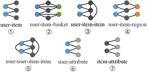
Although the above models can greatly capture the interaction information between users and items, they ignore geographical context of items that are closely related to user activities (Figure 1).

Figure 1. An illustration of graph structures in Table 1.

2.3. Personalized recommendations with geolocation

With the popularity of smart wear and electronic mobile devices, location-based services are becoming an integral part of people’s lives. A growing number of Internet applications are recording users’ experiences by collecting location information. Recent studies have revealed that human activities are influenced by geographic space. In addition, these activities have been observed to follow a certain spatial pattern.

By introducing geographical data, we can better infer a user’s preferences and accurately predict the items and locations that users would like to visit (Yuan, Raubal, and Liu 2012; Huang and Wong 2015). A growing body of work has paid attention to the location information of users and items (Zhang and Chow 2013; Zhang, Chow, and Li 2015; Zhao et al. 2020), which helps improve the accuracy of recommendations. The above works still fail to both capture higher-order interaction information between users and items and utilize item locations. Consequently, Location-aware neural graph CF (LA-NGCF) introduces the spatial distances of items into GNN to capture higher-order interaction information (Li et al. 2022). However, determining how to use spatial context, such as geographical regions, to improve the performance of graph-based CF models is a challenging yet promising task.

The above models that are closely related to the study are compared in Table 1, including GNN-based CF models without geolocation (section 2.2) and with geolocation (the LA-NGCF model), and the proposed model (RA-NGCF). Compared with LA-NGCF that utilizes the spatial distances of items into GNN model, this paper will use geographical region entities to capture the implicit spatial preferences of users.

Table 1. Comparison of GNN-based models, where NGCF-style models (NGCF, BasConv, LA-NGCF and RA-NGCF) are highlighted, and graph structures are illustrated in Figure 1.

Model	Embedding		Graph structure	Encoder	Score function
	User & item	Other
GC-MC (van den Berg, Kipf, and Welling 2017)	${\mathit{e}}_u,{\mathit{e}}_i\in {\mathbb{R}}^d$	–	①	GCN	${\mathit{e}}_u^T{W}_r{\mathit{e}}_i$
Spectral CF (Zheng et al. 2018)	${\mathit{e}}_u,{\mathit{e}}_i\in {\mathbb{R}}^d$	–	①	ResGCN	${\mathit{e}}_u^T{\mathit{e}}_i$
MCCF (Wang et al. 2020)	${\mathit{e}}_u,{\mathit{e}}_i\in {\mathbb{R}}^d$	–	①	Multi-CGCN	$MLP\left({\mathit{e}}_u\parallel {\mathit{e}}_i\right)$
LightGCN (He et al. 2020)	${\mathit{e}}_u,{\mathit{e}}_i\in {\mathbb{R}}^d$	–	①	LightGCN	${\mathit{e}}_u^T{\mathit{e}}_i$
DG-ENN (Guo et al. 2021)	${\mathit{e}}_u,{\mathit{e}}_i\in {\mathbb{R}}^d$	Attribute: ${\mathit{e}}_{A_u}\in {\mathbb{R}}^d$ ${\mathit{e}}_{A_i}\in {\mathbb{R}}^d$	⑤⑥⑦	LightGCN	$MLP\left({\mathit{e}}_u\parallel {\mathit{e}}_i\parallel {\mathit{e}}_{A_u}\parallel {\mathit{e}}_{A_i}\right)$
NGCF (Wang et al. 2019)	${\mathit{e}}_u,{\mathit{e}}_i\in {\mathbb{R}}^d$	–	①	ResGCN with user-item interaction	${\mathit{e}}_u^T{\mathit{e}}_i$
BasConv (Liu et al. 2020)	${\mathit{e}}_u,{\mathit{e}}_i\in {\mathbb{R}}^d$	Basket: ${\mathit{e}}_b\in {\mathbb{R}}^d$	②	ResGCN with user-item, user-basket, basket-item interaction	$({\mathit{e}}_u\oplus {\mathit{e}}_b{)}^T{\mathit{e}}_i$
LA-NGCF (Li et al. 2022)	${\mathit{e}}_u,{\mathit{e}}_i\in {\mathbb{R}}^d$	–	③	ResGCN with user-item, item-item interaction and geo-weights	${\mathit{e}}_u^T{\mathit{e}}_i$
RA-NGCF (Ours)	${\mathit{e}}_u,{\mathit{e}}_i\in {\mathbb{R}}^d$	Region: ${\mathit{e}}_r\in {\mathbb{R}}^d$	④	ResGCN with user-item, region-item interaction	${\mathit{e}}_u^T\left({\mathit{e}}_i\oplus {\mathit{e}}_r\right)$

In the table, $\parallel$ denotes the concatenation; $\oplus$ denotes the element-wise addition; ResGCN is a variant of GCN where the embeddings $\left\{{\mathit{e}}^{\left(0\right)},\dots ,{\mathit{e}}^{\left(L\right)}\right\}$ learned by different layers are concatenated; Multi-CGCN (Multi-component GCN) is a variant of GCN with a decomposer for user/item-specific component and a combiner for user/item-aggregated component; LightGCN is a variant of GCN without feature transformation and nonlinear activation.

3. Region-aware neural graph collaborative filtering

This section introduces the proposed model, region-aware neural graph CF model (RA-NGCF). As shown in Figure 2, RA-NGCF consists of three components: building the user-item-region graph, aggregating information between neighbor nodes, and predicting user preferences.

Figure 2. Region-aware neural graph CF model.

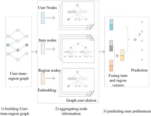
The first component is used for characterizing relationships among users, items, and regions by building a user-item-region graph based on visit history and spatial location. The second component aims to learn the features of each node by propagating and learning from its neighbor nodes with a GNN. The third component predicts user preferences by fusing the vectors of users, items, and regions.

3.1. Building user-item-region graph

The model first defines the geographical regions of items for characterizing the relationships among users, items, and regions, as these regions can present spatial features. In previous works, two types of regional definition strategies have been widely used to divide spatial areas into regions. One straightforward method is to divide the whole area into equally sized grids. Generally, the spatial patterns of human activity presented by spatial features of items are not typically grid-like. Therefore, dividing the area into grid regions is not appropriate for presenting user activities. An alternative strategy is to use administrative divisions, such as zip code, census tract, etc. Compared with the grid regions, administrative regions generally have high-level intra-regional connectivity because people are closely connected within a region. The selection of regional definition strategies is discussed in Section 5.3.

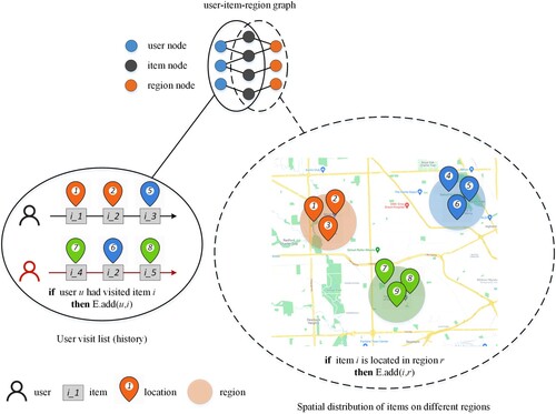
After determining the region corresponding to each item, the relationships among users, items, and regions are constructed as shown in Figure 3. In this study, these correlations are represented by a graph in which users, items and, regions are presented by three types of nodes, as shown in Figure 3. The graph is defined as ${\mathit{G}}_{uir}=\left(\mathit{U}\cup \mathit{I}\cup \mathit{R},{\mathit{W}}^{ui},{\mathit{W}}^{ir}\right)$, where U denotes the set of user nodes, $\mathit{I}$ denotes the set of items, and $R$ denotes the set of regions (Algorithm 1, line 1). In addition, ${\mathit{W}}^{ui}$ presents the binary weight matrix of the edges between users and items, while ${\mathit{W}}^{ir}$ denotes the binary weight matrix of the edges between items and regions. ${\mathit{W}}^{ui}$ matrix is used to present the historical preferences between users and items. In ${\mathit{W}}_{a,b}^{ui}$, the element ${\mathit{W}}^{\mathit{u}i}$, is set to 1 if user $a$ has visited item b; otherwise, it is set to 0 (Algorithm 1, line 3–7). ${\mathit{W}}^{ir}$ is used to present the relationships between items and regions. ${\mathit{W}}_{a,b}^{ir}$ is set to 1 if item $a$ is located in region $b$; otherwise, it is set to 0 (Algorithm 1, line 8–12).

Figure 3. The user-item-region graph, where the construction process of user-item edges and item-region edges are illustrated in the left part and the right part, respectively.

Table

Algorithm 1 User-item-region graph construction

Input: User set $\mathrm{U}=\left\{u_1,\dots ,u_n\right\}$; item set $\mathrm{I}=\left\{i_1,\dots ,i_m\right\}$; region set $\mathrm{R}=\left\{r_1,\dots ,r_o\right\}$; Output: User-item-region graph G = (V, E) 01: $\mathrm{V}=\mathrm{U}\cup \mathrm{I}\cup \mathrm{R}$ 02: $\mathrm{E}=\mathrm{\varnothing }$ 03: for $\left[u,i\right]\in \mathrm{U}\times \mathrm{I}$ do 04:  if $u$ had visited $i$ then 05:      E.add($u,i$) 06:  end if 07: end for 08: for $\left[i,r\right]\in \mathrm{I}\times \mathrm{R}$ do 09:  if $i$ is located in $r$ then 10:      E.add($i,r$) 11:  end if 12: end for 13: return G = (V, E)

3.2. Aggregating neighbor node information

The user-item-region graph consists of two types of edges: edges between user and item (UIE) and edges between item and region (IRE). The UIEs represent interactions between users and items, and IREs represent interactions between regions and items. Interactions between users and regions are not explicitly described in the graph. Considering that user activities usually present a spatial pattern, the interactions between users and regions are captured by propagating information on the three types of nodes.

The initial representations of users, items, and regions are formalized as Equations (1), (2), and (3), respectively. In the equations, ${\mathit{E}}_u\in R^{d\times n},{\mathit{E}}_i\in R^{d\times m},and{\mathit{E}}_r\in R^{d\times o}$ denote the vector sets of users, items, and regions, respectively, where $\mathit{d}$ denotes the dimension size of these vectors. (1) ${\mathit{E}}_u=\left[{\mathit{e}}_1,{\mathit{e}}_2\dots {\mathit{e}}_{n-1},{\mathit{e}}_n\right]$(1) (2) ${\mathit{E}}_i=\left[{\mathit{e}}_1,{\mathit{e}}_2\dots {\mathit{e}}_{m-1},{\mathit{e}}_m\right]$(2) (3) ${\mathit{E}}_r=\left[{\mathit{e}}_1,{\mathit{e}}_2\dots {\mathit{e}}_{o-1},{\mathit{e}}_o\right]$(3)

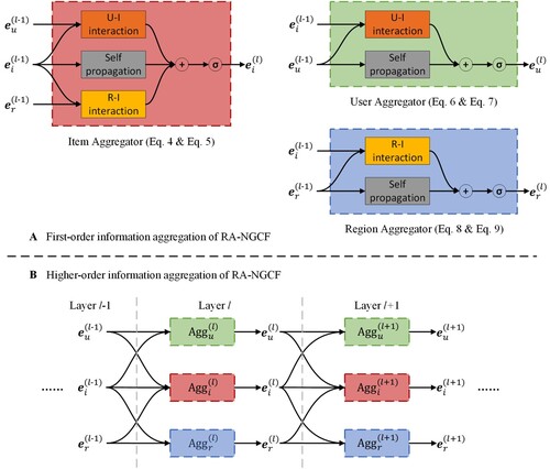
In the user-item-region graph, an item node is connected to both user and region nodes, which can directly learn region features from neighbor regions and user features from neighbor user nodes. Then, two kinds of learned features are propagated to the neighbor nodes. The updating of node vectors can be performed by three aggregators, including item aggregator, user aggregator and region aggregator, to update item node vectors, user node vectors, and region node vectors, respectively. The aggregators are illustrated in Figure 4.

• Item Aggregator. Item nodes are directly connected to two types of nodes, namely, user nodes and region nodes. The UIE presents interactions between items and users, thus implicitly reflecting user preferences. The IRE presents the relationships between items and regions, thus capturing the geographical characteristics of items. To fuse the above two types of information in the process of information propagation, Equation (4) is designed for fusing information collected from neighboring nodes. (4) ${\mathit{m}}_{i\leftarrow u,r}={\displaystyle \frac{1}{\sqrt{\left|N_u\right|\left|N_i\right|\left|N_r\right|}}\left({\mathit{W}}_1({\mathit{e}}_u+{\mathit{e}}_r)+{\mathit{W}}_2\left({\mathit{e}}_i\otimes {\mathit{e}}_u+{\mathit{e}}_i\otimes {\mathit{e}}_r\right)\right)}$(4) where $\otimes$ denotes element-wise multiplication. $N_u$, $N_i$, and $N_r$ denote the number of direct-connect neighbor nodes of users, items, and regions, respectively. ${\mathit{m}}_{i\leftarrow u,r}$ is a vector that an item collected from its neighbor nodes. It contains two types of information: original information in the neighbor nodes and information that the neighbor nodes obtained from their neighbor nodes. ${\mathit{W}}_1({\mathit{e}}_u+{\mathit{e}}_r)$ denotes the feature information of user nodes and region nodes collected by items from neighbor nodes; ${\mathit{W}}_2\left({\mathit{e}}_i\otimes {\mathit{e}}_u+{\mathit{e}}_i\otimes {\mathit{e}}_r\right)$ contains two parts: ${\mathit{e}}_i\otimes {\mathit{e}}_u$ denotes the interaction information between the item and the user, from which the user’s interest preferences can be exploited. ${\mathit{e}}_i\otimes {\mathit{e}}_r$ denotes the interaction information between the item and the region, which propagates the region feature into item vectors. ${\mathit{W}}_1,{\mathit{W}}_2\in R^{d^{\mathrm{\prime }}\times d}$ are two training parameter matrices. $d^{\mathrm{\prime }}$ denotes the dimension size of the aggregated neighbor node vectors.

  After collecting feature information from the neighbor nodes, the original item vector representation can be updated with the received information, which can be derived as Equation (5): (5) ${\mathit{e}}_i^{\left(1\right)}=LeakyReLU\left({\mathit{m}}_{i\leftarrow i}+\sum _{u,r\in N_i}{\mathit{m}}_{i\leftarrow u,r}\right)$(5) where LeakyReLU() is the activation function; ${\mathit{m}}_{i\leftarrow i}$ is the preserved feature information, which can be calculated by ${\mathit{m}}_{i\leftarrow i}=W_3{\mathit{e}}_i$. The process of the item vector update can be divided into two steps. The first step is to collect feature information from neighbor nodes, and the second step is to aggregate the information collected from these nodes. In the collection process, both the information of the neighbor nodes and the information of the item’s interaction with them is added. In the process of information aggregation, the characteristics of the item are preserved, and the information collected from neighbor nodes is fused, which can reduce the possibility of over-fitting when the node information propagates deeply through multiple layers. After the information collection and information aggregation from the neighbor nodes, the vector representation of the item contains both the region feature of the item and the preferences of users. Then, the region feature in items is propagated to user nodes, thus enabling the user’s vector to become aware the region feature of the items. At the same time, the user preference information in items is propagated to vectors of regions so that region vectors can capture the preferences of users.

• User Aggregator. In the built user-item-region graph, both user nodes and region nodes have only one type of neighbor node. The update process of both user and region vectors is similar to the update process of item vectors, which consists of two steps: information collection from neighbor nodes and information aggregation. The user vectors that collect information from neighbor nodes are derived as: (6) ${\mathit{m}}_{u\leftarrow i}={\displaystyle \frac{1}{\sqrt{\left|N_u\right|\left|N_i\right|}}\left({\mathit{W}}_1{\mathit{e}}_i+{\mathit{W}}_2\left({\mathit{e}}_i\otimes {\mathit{e}}_u\right)\right)}$(6) where ${\mathit{m}}_{u\leftarrow i}$ presents the information that users collected from their neighbor nodes; the aggregation process is defined as Equation (7): (7) ${\mathit{e}}_u^{\left(1\right)}=LeakyReLU\left({\mathit{m}}_{u\leftarrow u}+\sum _{i\in N_u}{\mathit{m}}_{u\leftarrow i}\right)$(7) where ${\mathit{e}}_u^{\left(1\right)}$ is the representation vectors of the user node after aggregating information from direct-connected neighbor nodes, in which ${\mathit{m}}_{u\leftarrow u}$ is used to preserve its own feature.

• Region Aggregator. The process of region nodes collecting information from neighboring nodes can be formalized as: (8) ${\mathit{m}}_{r\leftarrow i}={\displaystyle \frac{1}{\sqrt{\left|N_r\right|\left|N_i\right|}}\left({\mathit{W}}_1{\mathit{e}}_i+{\mathit{W}}_2\left({\mathit{e}}_i\otimes {\mathit{e}}_r\right)\right)}$(8) where ${\mathit{m}}_{r\leftarrow i}$ is the feature information that regions collected from their neighbor items, which represents the characteristics of region $r$. For region r, its features can be calculated as Equation (9): (9) ${\mathit{e}}_r^{\left(l\right)}=LeakyReLU\left({\mathit{m}}_{r\leftarrow r}+\sum _{i\in N_r}{\mathit{m}}_{a\leftarrow i}\right)$(9) where ${\mathit{m}}_{r\leftarrow r}$ represents the feature information of the region itself, and ${\mathit{e}}_r^{\left(l\right)}$ is the representation of the region vector after l-th iteration. At this moment, the region vector contains the feature information of regions, and it also obtains the user’s preference information learned from items.

This study designed a three-layer GNN for information propagation and concatenates the vectors of each layer to obtain the final vector representation of users, items, and regions as follows. (10) ${\mathit{e}}_u^{\ast }={\mathit{e}}_u^{\left(0\right)};\dots ;{\mathit{e}}_u^{\left(l\right)}$(10) (11) ${\mathit{e}}_i^{\ast }={\mathit{e}}_i^{\left(0\right)};\dots ;{\mathit{e}}_i^{\left(l\right)}$(11) (12) ${\mathit{e}}_r^{\ast }={\mathit{e}}_r^{\left(0\right)};\dots ;{\mathit{e}}_r^{\left(l\right)}$(12)

Figure 4. Illustration of information aggregation. On the part A, three aggregators with examples of aggregating the l-th embedding are presented. The part B shows how to introduce aggregators mentioned in part A to learn higher-order embeddings of nodes.

3.3. Predicting and optimizing

Personalized recommendations based on CF usually score user vectors and item vectors to infer and predict user preferences. In this study, we can infer users’ preferences by using three types of vectors: user vectors, item vectors, and region vectors. In the user-item-region graph, each item node is connected to the unique region node, that is, all item nodes in the same area are connected to the same region node. Thus, a region vector should reflect the common characteristics of items in the region. RA-NGCF fuses the region vectors and item vectors before predicting user preferences. Then, fused item vectors are used to predict user preferences. The fusing process is performed with Equation (13). (13) ${\mathit{e}}_{i-r}^{\ast }={\mathit{e}}_i^{\ast }\oplus {\mathit{e}}_r^{\ast }$(13) where $e_{i-r}^{\ast }$ denotes the fused vector representation of items. In addition, ⊕ denotes the element-wise addition of vectors. Besides addition operation, multiplication operation or subtraction operation can be applied to fuse the two vectors. Extensive experiments are discussed in Section 5.1.

Then, the vector dot product is calculated to score the similarity between user vectors and item vectors, which is defined in Equation (14). Compared with cosine similarity, the dot product of vectors can simplify the computational cost. Given the strategy of introducing parameter regularization and vector normalization in the implementation of the model, the dot product of vectors and cosine similarity is consistent in determining the relative similarity between items and a given user. (14) ${\hat{y}}_{\left(u,i-r\right)}={\mathit{e}}_u^{\ast T}{\mathit{e}}_{i-r}^{\ast }$(14) where ${\hat{y}}_{\left(u,i-r\right)}$ is the final preference score of user u to item i.

The BPR loss function (Rendle et al. 2009) is applied to learn the optimization objective of the model, and the loss function of RA-NGCF is defined as follows: (15) $Loss=\sum _{\left(u,i,j\right)\in O}-\ln \sigma \left({\hat{y}}_{u,i-r}-{\hat{y}}_{u,j-r}\right)+\lambda {\mathrm{\Theta }}_2^2$(15) where $i-r$ denotes a positive case and $j-r$ denotes a negative case. Finally, we summarize the training procedure of our proposed RA-NGCF model in Algorithm 2.

Table

Algorithm 2 Training of RA-NGCF

Require User-item-region graph G = (V, E) and nodes features obtained via Eq. 1, Eq. 2 and Eq. 3 01: while not converge do 02:  Update item, user and region embeddings via Eq. 5, Eq. 7 and Eq. 9, respectively 03:  Obtain the final user, item and region embeddings via Eq. 10, Eq. 11 and Eq. 12, respectively 04:  Sample a batch ${\mathit{S}}_T$ from training set 05:  Compute the optimization objective L via Eq. 15 on batch ${\mathit{S}}_T$ 06:  Update aggregators parameters W in Eq. 4–Eq. 9 07: end while

4. Experiments and results

This section introduces the details of the dataset selection for our experiments (including dataset processing methods), evaluation metrics, and parameter settings.

4.1. Dataset

The dataset used in this study is built from ‘Yelp Dataset Challenge 2019’ downloaded from https://www.yelp.com/dataset/. The dataset collected user reviews from Yelp, including user description, user check-ins, user reviews, and item descriptions. We plotted the spatial distribution of items in the dataset, as presented in Figure 5. As seen from the figure, the spatial distribution of items is not uniform, revealing significant spatial heterogeneity. In addition, the POIs visited by users are spatially aggregated, which suggests that the introduction of geographical regions should facilitate in predicting users’ preferences.

Figure 5. Spatial distribution of items accessed by several users in the Yelp dataset.

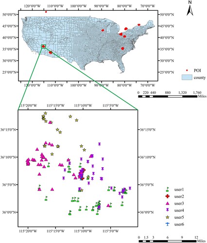
In the following experiments, we use the user ID in the user’s check-in file and the ID of the item visited by the user. We also look for the corresponding postal code in the item files according to IDs of the items. The postal code can be used to identify spatial regions in which items are located. The downloaded raw data form a user review dataset, in which users’ check-ins are very sparse. Consequently, users with less than 20 check-ins and items with less than 20 visits are removed, and the descriptive statistics of the dataset after processing are shown in Table 2.

Table 2. Descriptive statistics of the dataset.

Dataset	#users	#itmes	#areas	#check-ins	Density
Yelp	24,357	18,544	2656	1,203,863	0.2665%

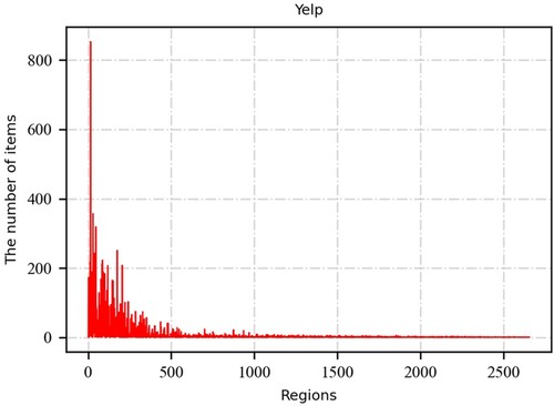
As shown in Table 2, the built dataset contains 24,357 users and 18,544 items, which are located in 2656 zip code regions. To observe the distribution of items across regions further, the number of items in each area is counted and plotted in Figure 6. The figure shows that the distribution of items in each region is very different. In addition, 211 regions contain more than 10 items, with a total of 14,063 items, thus accounting for more than 75% of all items. The remaining 4481 items are located in 2445 regions. This outcome suggests that the items are distributed in a significantly long-tail pattern. This distribution pattern indicates that user activities are highly localized, and the region feature should be valued for personalized recommendation tasks.

Figure 6. The distribution of the number of items in each region.

4.2. Experiment setting

Baselines. Three classical CF models are employed as our baselines, i.e. MF (Rendle et al. 2009), NeuMF (He et al. 2017) and NGCF (Wang et al. 2019). Here MF is a matrix factorization model optimized by the Bayesian personalized ranking (BPR) loss function, NeuMF is an advanced neural CF model, and NGCF is a GNN-based CF model that captures higher-order information between the user and item.

Evaluation metrics. To evaluate the performance of the proposed model, this study takes recall@K, ndcg@K, and hit@K as evaluation metrics. Recall@K considers that the percentage of visiting POIs can emerge in the top K recommended POIs. Hit@K considers whether the relevant items are retrieved within the top K positions of the recommendation list. Ndcg@K measures the relative orders among positive and negative items within the top K of the ranking list (Wang et al. 2019). In the experiments, K is set to 20, which is the same as the set value in the experiment in the NGCF work (Wang et al. 2019).

Implementation details. The proposed model in this study is implemented with Python and TensorFlow (Abadi et al. 2016). In the experiments, the size of all user, item, and region vectors are set to 64 and are randomly initialized with the Xavier initializer (Glorot and Bengio 2010). We divide the dataset into three parts: training set, testing set, and validation set. The number ratio of these parts is 8:1:1. The proposed model is trained for 400 epochs on the training dataset.

4.3. Results

Five models, including three baseline models and two variants of the proposed model, are performed on the dataset to examine the performance of the proposed model. The experimental results are reported in Table 3, where RA-NGCF denotes the proposed model (Wang et al. 2019). A-NGCF is a variant of RA-NGCF in which only the scores of user vectors and item vectors are taken into consideration in the recommended prediction. In addition, A-NGCF does not fuse item and region vectors by ignoring Equation (14) in the predictive user preference component.

Table 3. Prediction accuracy of models.

Model	Recall@20	Hit@20	NDCG@20
MF	0.0778	0.4543	0.1401
NeuMF	0.0629	0.3572	0.1073
NGCF	0.0973	0.5462	0.1622
A-NGCF	0.0976	0.5491	0.1623
RA-NGCF	0.1029	0.5617	0.1688
%Improv.	5.76	2.84	3.91

As shown in Table 3, RA-NGCF achieves the best performance. Although A-NGCF does not combine region node vectors with item node vectors to predict user preferences, it achieves better performance than the baseline models, NGCF. The user-item-region graph involves region nodes, and the process of node information propagation captures the interaction information between users and items, and the geographical features between items and regions.

The performance of the proposed model, RA-NGCF, has been improved, as indicated by three evaluation metrics, namely, recall@20, hit@20, and ndcg@20. The most significant improvement was observed in the metric of recall@20, which was 5.76% higher than the strongest baseline model. The improvements on hit@20 and ndcg@20 are 2.84% and 3.91%, respectively. Compared with A-NGCF, the results suggest that the geographical characteristics of items in RA-NGCF are effectively propagated with the user-item-region graph. In general, we argue that region entities are important in the personalized recommendation task. We also believe that incorporating the region feature as attribute information into the vector representation of items is a promising approach to improving the performance of the model.

To observe the contribution of the region feature in the proposed model further, we randomly select some regions in the experiments. Then, we test the prediction accuracy of the proposed model and the baseline model and plot the Recall@20 values of selected regions in Figure 7.

Figure 7. Model performance of those regions.

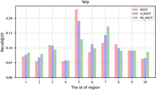
In Figure 7, the NGCF results are marked in red, and the prediction accuracies fluctuate greatly between regions, which may be because the NGCF model does not take into account the region features of the items. The accuracies may have fluctuated because the items are not uniformly distributed over the regions, thus resulting in spatial heterogeneity model performance. Hence, the NGCF model has performed well in certain regions and poorly in others. The results of the RA-NGCF model are shown in green, and their performance is well balanced. They suggest that the introduction of region nodes can improve the balance of spatial distribution.

5. Discussion

5.1. Fused presentation vectors of regions and items

The proposed model predicts user preferences by scoring user vectors and fused item vectors, where the fused item vectors are fused with raw item vectors and region vectors. As mentioned in Section 3.3, some operations can be used to combine item and region vectors. In this section, experiments conducted on several widely used vector fusion methods are presented, and the results are listed in Table 4. As shown in the table, the subtraction operation achieves the best results. Meanwhile, the addition operation has the second best results, while the multiplication operation has the worst results. We use the most common operation, the addition operation, to fuse the two types of vectors in other experiments of this study.

Table 4. Comparison of different vector fusing operations; the best results are shown in bold.

Operation	Recall@20	Hit@20	NDCG@20
Addition	0.1029	0.5617	0.1688
Subtraction	0.1034	0.5658	0.1690
Multiplication	0.0936	0.5325	0.1556

5.2. Experiments on sparsity data

To illustrate the importance of regional information in the recommendation task further, we conduct experiments on datasets with different sparsity, and the results are shown in Table 5. Specifically, we randomly select items from the used dataset mentioned in Section 4. Then, we randomly remove the visit records from the training set. The percentage in Table 5 indicates the proportion of randomly selected items omitted. As shown in the table, the sparser the dataset is, the worse the performance of the NGCF model and the RA-NGCF model will be. The RA-NGCF model always outperforms the NGCF model, which indicates that RA-NGCF is robust and that fusing regional information can improve the performance of the model.

Table 5. Performance of NGCF model and RA-NGCF model under different sparse data; the best results are shown in bold.

Percentage	NGCF		RA-NGCF
	Recall@20	NDCG@20	Recall@20	NDCG@20
0	0.0973	0.1622	0.1029	0.1688
5	0.0950	0.1607	0.1006	0.1671
10	0.0948	0.1619	0.0982	0.1657
15	0.0903	0.1576	0.0938	0.1637
20	0.0876	0.1556	0.0904	0.1607

5.3. Grid-based regions

As most of the spatial applications meet the modified area unit problem (MAUP) (Xiong et al. 2019), the performance of the proposed model may be affected by different region division strategies. The section will examine the impact of region division strategies on the performance of the model.

In this section, we perform experiments with two regions and define the methods mentioned in Section 3.1. Then, we list the results in Table 6. For grid-based regions, two spatial sizes, 500*500 and 1,000*1000 are selected, and their results are marked as grid (500*500) and grid (1000*1000), respectively. The zip code denotes defined regions by post codes, which is adopted in several spatial applications.

Table 6. Performance of RA-NGCF model under different regional division methods; the best results are shown in bold.

Region	Recall@20	Hit@20	NDCG@20
Grid (500, 500)	0.1041	0.5701	0.1707
Grid (1000, 1000)	0.1037	0.5658	0.1705
Zip code	0.1029	0.5617	0.1688

As shown in Table 6, different region types affect the performance of the proposed model. The best prediction performance is obtained when dividing the spatial area into a 500*500 grid regions. The proposed method also suffers from the MAUP issue (Wong 2009), and the grid size will affect the prediction accuracies when the grid-based method is applied. We argue that if the region is too large, the region will have too many items, and the items may be too ‘noisy.’ Hence, the regional nature of the items is not capture well. Meanwhile, if the region is too small, then the model will have too many regions, which will greatly increase the nodes of the model. All results are superior to the baseline models mentioned in Section 4, thus indicating that the model is robust.

The regions based on administrative areas are more conducive to understanding human activities and are expected to be more easily integrated with existing spatial applications. The rest of the experiments in this study are designed to define region objects with a widely used administrative area, the zip code region.

6. Conclusions

By introducing geographical entities, this study develops an optimized personalized recommendation model, RA-NGCF. The proposed model first uses the user-item-region graph to characterize the relationships among users, items, and regions. Then, it projects items into geographical regions and designs a GNN to propagate the features of users, items, and regions. Experimental results show that RA-NGCF outperforms baseline models. Specifically, the introduction of geographical regions of items not only improves the overall effectiveness of the model but also alleviates the impact of the uneven spatial distribution of items. This study provides a new approach for optimizing personalized recommendation and a methodological reference of facilitating geographical information to spatial applications.

A challenge of this study is that some regions have few items, thus making that the proposed model capture the characteristics of those regions insufficiently. More machine learning techniques, such as transfer learning strategies, can be introduced into the proposed models to improve recommendation accuracy in those regions. In addition, the proposed model faces the challenge from the modified area unit problem (MAUP), i.e. different spatial scale levels and region shapes may affect the performance of the proposed model, and the challenge deserve to be further considered.

Disclosure statement

No potential conflict of interest was reported by the author(s).

References

- Abadi, M., P. Barham, J. Chen, Z. Chen, A. Davis, J. Dean, M. Devin, et al. 2016. “TensorFlow: A System for Large-Scale Machine Learning.” In: Proceedings of the 12th USENIX Symposium on Operating Systems Design and Implementation, OSDI 2016, 265–283.
- Baluja, S., R. Seth, D. S. Sivakumar, Y. Jing, J. Yagnik, S. Kumar, D. Ravichandran, and M. Aly. 2008. “Video Suggestion and Discovery for You Tube: Taking Random Walks Through the View Graph.” In: Proceeding of the 17th International Conference on World Wide Web 2008, WWW’08, 895–904.
- Bao, Y., Z. Huang, L. Li, Y. Wang, and Y. Liu. 2021. “A BiLSTM-CNN Model for Predicting Users’ Next Locations Based on Geotagged Social Media.” International Journal of Geographical Information Science 35 (4): 639–660.
- Botangen, K. A., J. Yu, Q. Z. Sheng, Y. Han, and S. Yongchareon. 2020. “Geographic-Aware Collaborative Filtering for Web Service Recommendation.” Expert Systems with Applications 151: 113347.
- Gambs, S., M. O. Killijian, and M. N. Del Prado Cortez. 2012. “Next Place Prediction Using Mobility Markov Chains.” Proceedings of the 1st Workshop on Measurement, Privacy, and Mobility, MPM’12, 0–5.
- Glorot, X., and Y. Bengio. 2010. “Understanding the Difficulty of Training Deep Feedforward Neural Networks.” Journal of Machine Learning Research 9: 249–256.
- Guo, W., R. Su, R. Tan, H. Guo, Y. Zhang, Z. Liu, R. Tang, and X. He. 2021. “Dual Graph Enhanced Embedding Neural Network for CTR Prediction.” In: Proceedings of the 27th ACM SIGKDD Conference on Knowledge Discovery & Data Mining, 496–504.
- Guo, Q., F. Zhuang, C. Qin, H. Zhu, X. Xie, H. Xiong, and Q. He. 2022. “A Survey on Knowledge Graph-Based Recommender Systems.” IEEE Transactions on Knowledge and Data Engineering 34 (8): 3549–3568.
- He, X., K. Deng, X. Wang, Y. Li, Y. D. Zhang, and M. Wang. 2020. “LightGCN: Simplifying and Powering Graph Convolution Network for Recommendation.” SIGIR 2020 - Proceedings of the 43rd International ACM SIGIR Conference on Research and Development in Information Retrieval, 639–648.
- He, X., M. Gao, M. Y. Kan, and D. Wang. 2017a. “BiRank: Towards Ranking on Bipartite Graphs.” IEEE Transactions on Knowledge and Data Engineering 29 (1): 57–71.
- He, X., Z. He, J. Song, Z. Liu, Y. G. Jiang, and T. S. Chua. 2018. “NAIS: Neural Attentive Item Similarity Model for Recommendation.” IEEE Transactions on Knowledge and Data Engineering 30 (12): 2354–2366.
- He, X., L. Liao, H. Zhang, L. Nie, X. Hu, and T.-S. S. Chua. 2017b. “Neural Collaborative Filtering.” 26th International World Wide Web Conference, WWW 2017, 173–182.
- Huang, Q., and D. W. S. Wong. 2015. “Modeling and Visualizing Regular Human Mobility Patterns with Uncertainty: An Example Using Twitter Data.” Annals of the Association of American Geographers 105 (6): 1179–1197.
- Jiang, Z., H. Liu, B. Fu, Z. Wu, and T. Zhang. 2018. “Recommendation in Heterogeneous Information Networks Based on Generalized Random Walk Model and Bayesian Personalized Ranking.” In: WSDM 2018 – Proceedings of the 11th ACM International Conference on Web Search and Data Mining, 288–296.
- Kipf, T. N., and M. Welling. 2017. “Semi-Supervised Classification with Graph Convolutional Networks.” 5th International Conference on Learning Representations, ICLR 2017 – Conference Track Proceedings, 1–13.
- Koren, Y., R. Bell, and C. Volinsky. 2009. “Matrix Factorization Techniques for Recommender Systems.” Computer 42 (8): 30–37.
- Li, W., X. Liu, C. Yan, G. Ding, Y. Sun, and J. Zhang. 2020. “STS: Spatial-Temporal-Semantic Personalized Location Recommendation.” ISPRS International Journal of Geo-Information 9 (9): 538.
- Li, S., C. Sun, R. Chen, X. Li, Q. Liang, J. Gong, and H. Yao. 2022. “Location-Aware Neural Graph Collaborative Filtering.” International Journal of Geographical Information Science 36 (8): 1550–1574.
- Liu, Y., and H. S. Seah. 2015. “Points of Interest Recommendation from GPS Trajectories.” International Journal of Geographical Information Science 29 (6): 953–979.
- Liu, Z., M. Wan, S. Guo, K. Achan, and P. S. Yu. 2020. “Basconv: Aggregating Heterogeneous Interactions for Basket Recommendation with Graph Convolutional Neural Network.” In: Proceedings of the 2020 SIAM International Conference on Data Mining. SIAM, 64–72.
- Liu, W., Z. J. Wang, B. Yao, and J. Yin. 2019. “Geo-ALM: POI Recommendation by Fusing Geographical Information and Adversarial Learning Mechanism.” IJCAI International Joint Conference on Artificial Intelligence, 2019-August, 1807–1813.
- Liu, Q., S. Wu, L. Wang, and T. Tan. 2016. “Predicting the Next Location: A Recurrent Model with Spatial and Temporal Contexts.” 30th AAAI Conference on Artificial Intelligence, AAAI 2016, 194–200.
- Mikolov, T., I. Sutskever, K. Chen, G. Corrado, and J. Dean. 2013. “Distributed Representations of Words and Phrases and Their Compositionality.” In: Advances in Neural Information Processing Systems, 3111–3119.
- Nikolakopoulos, A. N., and G. Karypis. 2019. “Recwalk: Nearly Uncoupled Random Walks for Top-n Recommendation.” WSDM 2019 – Proceedings of the 12th ACM International Conference on Web Search and Data Mining, 150–158.
- Rendle, S. 2010. “Factorization Machines.” In: 2010 IEEE International Conference on Data Mining. IEEE, 995–1000.
- Rendle, S., C. Freudenthaler, Z. Gantner, and L. Schmidt-Thieme. 2009. “BPR: Bayesian Personalized Ranking from Implicit Feedback.” In: The 25th Conference on Uncertainty in Artificial Intelligence, UAI 2009, 452–461.
- Shi, C., B. Hu, W. X. Zhao, and P. S. Yu. 2019. “Heterogeneous Information Network Embedding for Recommendation.” IEEE Transactions on Knowledge and Data Engineering 31 (2): 357–370.
- van den Berg, R., T. N. Kipf, and M. Welling. 2018. “Graph Convolutional Matrix Completion.” In: Proceedings of the 24th ACM SIGKDD International Conference on Knowledge Discovery & Data Mining. London, UK, 32.
- Wang, X., X. He, M. Wang, F. Feng, and T. S. Chua. 2019a. “Neural Graph Collaborative Filtering.” In: SIGIR 2019 – Proceedings of the 42nd International ACM SIGIR Conference on Research and Development in Information Retrieval, 165–174.
- Wang, S., L. Hu, Y. Wang, X. He, Q. Z. Sheng, M. A. Orgun, L. Cao, F. Ricci, and P. S. Yu. 2021. “Graph Learning Based Recommender Systems: A Review.” In: IJCAI International Joint Conference on Artificial Intelligence, 4644–4652.
- Wang, X., R. Wang, C. Shi, G. Song, and Q. Li. 2020. “Multi-Component Graph Convolutional Collaborative Filtering.” In: Proceedings of the AAAI Conference on Artificial Intelligence, 6267–6274.
- Wang, X., D. Wang, C. Xu, X. He, Y. Cao, and T.-S. Chua. 2019b. “Explainable Reasoning Over Knowledge Graphs for Recommendation.” Proceedings of the AAAI Conference on Artificial Intelligence, 33, 5329–5336.
- Wong, D. 2009. “The Modifiable Areal Unit Problem (MAUP).” The SAGE Handbook of Spatial Analysis, 105–123.
- Wu, J., X. Wang, F. Feng, X. He, L. Chen, J. Lian, and X. Xie. 2021. “Self-Supervised Graph Learning for Recommendation.” SIGIR 2021 – Proceedings of the 44th International ACM SIGIR Conference on Research and Development in Information Retrieval, 726–735.
- Xiao, S., Y. Shao, Y. Li, H. Yin, Y. Shen, and B. Cui. 2022. “LECF: Recommendation via Learnable Edge Collaborative Filtering.” Science China Information Sciences 65 (1): 112101.
- Xiong, C., A. Srivastava, R. Kannan, O. Damle, V. Prasanna, and E. Southers. 2019. “On Predicting Crime with Heterogeneous Spatial Patterns: Methods and Evaluation.” GIS: Proceedings of the ACM International Symposium on Advances in Geographic Information Systems, 43–51.
- Yang, J. H., C. J. Wang, C. M. Chen, and M. F. Tsai. 2018. “HoP-Rec: High-Order Proximity for Implicit Recommendation.” RecSys 2018 – 12th ACM Conference on Recommender Systems, 140–144.
- Yang, W., Y. Zhao, D. Wang, H. Wu, A. Lin, and L. He. 2020. “Using Principal Components Analysis and IDW Interpolation to Determine Spatial and Temporal Changes of Surfacewater Quality of Xin’Anjiang River in Huangshan, China.” International Journal of Environmental Research and Public Health 17 (8): 2942.
- Yin, H., W. Wang, H. Wang, L. Chen, and X. Zhou. 2017. “Spatial-Aware Hierarchical Collaborative Deep Learning for POI Recommendation.” IEEE Transactions on Knowledge and Data Engineering 29 (11): 2537–2551.
- Yuan, Y., M. Raubal, and Y. Liu. 2012. “Correlating Mobile Phone Usage and Travel Behavior – A Case Study of Harbin, China.” Computers, Environment and Urban Systems 36 (2): 118–130.
- Zhang, J. D., and C. Y. Chow. 2013. “iGSLR: Personalized Geo-Social Location Recommendation – A Kernel Density Estimation Approach.” GIS: Proceedings of the ACM International Symposium on Advances in Geographic Information Systems, 324–333.
- Zhang, J. D., C. Y. Chow, and Y. Li. 2015. “IGeoRec: A Personalized and Efficient Geographical Location Recommendation Framework.” IEEE Transactions on Services Computing 8 (5): 701–714.
- Zhang, S., H. Tong, J. Xu, and R. Maciejewski. 2019a. “Graph Convolutional Networks: A Comprehensive Review.” Computational Social Networks 6: 1. doi:10.1186/s40649-019-0069-y.
- Zhang, Y., C. Yin, Q. Wu, Q. He, and H. Zhu. 2019b. “Location-Aware Deep Collaborative Filtering for Service Recommendation.” IEEE Transactions on Systems, Man, and Cybernetics: Systems 51 (6): 3796–3807.
- Zhao, G., P. Lou, X. Qian, and X. Hou. 2020. “Personalized Location Recommendation by Fusing Sentimental and Spatial Context.” Knowledge-Based Systems 196: 105849.
- Zhao, P., A. Luo, Y. Liu, J. Xu, Z. Li, F. Zhuang, V. S. Sheng, and X. Zhou. 2022. “Where to Go Next: A Spatio-Temporal Gated Network for Next POI Recommendation.” IEEE Transactions on Knowledge and Data Engineering 34 (5): 2512–2524.
- Zheng, L., C. T. Lu, F. Jiang, J. Zhang, and P. S. Yu. 2018. “Spectral Collaborative Filtering.” RecSys 2018 – 12th ACM Conference on Recommender Systems, 311–319.