Segmentation of the communication tower and its accessory equipment based on geometrical shape context from 3D point cloud

ABSTRACT

Communication tower (CT) and its accessory equipment (AE) such as radio frequency equipment (RFE) and antenna, are essential in providing highspeed and stable mobile network services. It is necessary to routinely monitor the security and stability of CT and AE for seamless communication. There is limited research on fine segmentation of communication base station objects. This paper proposes a method for accurately segmenting the point cloud of the CT and AE from Terrestrial Laser Scanning (TLS) data. At first, the CT point cloud is accurately segmented based on region growing and Random Sample Consensus (RANSAC). Then, the point cloud of pole-shaped apart is extended to a certain distance to obtain the buffer point cloud containing AE. Normal Differential (ND) clustering is employed to obtain several groups of clusters containing planes, and calculate each plane's filling rate and size. Finally, the cluster type (such as antenna, RFE, or other) is distinguished. The experimental results demonstrate that the point-based average F1-score of CTs is 98. 70%, the point-based and object-based average F1-scores of antennas are 96. 09% and 97. 93%, and the corresponding values for the RFE are 89. 89% and 90. 00%, respectively, indicating the optimal performance of the proposed method.

KEYWORDS:

• Communication tower (CT)
• radio frequency equipment (RFE)
• antenna
• segmentation
• point cloud

1. Introduction

In the past decade, wireless network technology has flourished and become an indispensable communication tool in people's lives (Ali et al. 2021; Pahlavan et al. 2020). Communication Towers (CTs), as the infrastructure of communication base stations, support wireless network technology by transmitting or receiving electromagnetic waves using accessory equipment (AE) such as radio frequency equipment (RFE) and antennas.

(a) The general background of the study

With the development of wireless technology and the Internet of Things (IoT), rapid and precise positioning, high-definition data, real-time transmission, and other requirements have put forward higher requirements for base station construction and security (Huo, Dong, and Beatty 2020; Motlagh, Taleb, and Arouk 2016; Huo et al. 2019). The need for RFE and antenna expansion is increasing day by day. However, various factors such as crustal movement, harsh climate, aging oxidation, and potential human damage may cause CTs to deform, tilt, or even collapse, degrading the regular operation of communication equipment(Wang et al. 2018; Meng 2018). The precise data of the CTs are required to calculate the inclination angle and settlement of the tower body, verify the safety and reliability of the CTs in time, and promote the service life of the CTs. Besides, It is necessary to accurately obtain the position and number of CTs and existing AE on the CT to reasonably layout and standardize the management of communication base stations (Gao, Zhao, and Shen 2019; Fu, Gao, and Zhao 2020).

Currently, the traditional detection methods of CTs and AE can be divided into artificial observation and real-time monitoring using advanced monitoring equipment (Zhang et al. 2021). Due to the difficulty of manual observation of some parameters, it is impossible to achieve comprehensive, timely, and accurate observation, and it is challenging to find problems in time. Although monitoring equipment can perform real-time safety monitoring of CTs and timely and effectively discover potential problems in CTs and AE, it cannot realize 3D visualization of CTs and AE.

(b) Related works

Light Detection and Ranging (LiDAR) can directly and quickly acquire high-density and high-precision 3D point clouds of surface features. This provides advantages like high accuracy, high penetration capability, and high data processing automation (Nowak, Orłowicz, and Rutkowski 2020). TLS can effectively solve the problems of low accuracy and minimal time efficiency of traditional detection methods, realize the 3D visualization of objects (Nowak, Orłowicz, and Rutkowski 2020).

Scholars have studied the LiDAR-based extraction of power towers. For example, Zhang et al. (Zhang et al. 2019) constructed a spatial hash matrix using a statistical method to store the point cloud after noise removal and identify the power tower point cloud by calculating the local distribution characteristics of the points within each hash grid and analyzing the grid features in horizontal and vertical directions. Zhao et al. (Zhao et al. 2020) extracted power tower point clouds by statistically characterizing the spatial distribution of point clouds in transmission corridors, including point cloud density, elevation histogram, terrain elevation distribution, and feature elevation distribution. Tan et al. (Tan et al. 2021) utilized the K-dimensional (Kd) tree segmentation method, region growing algorithm, and Random Sample Consensus (RANSAC) in turn for coarse and fine extraction of power tower point cloud. Tan et al. (Tan et al. 2021) proposed a power line extraction algorithm based on Entropy-Weighting Feature Evaluation (EWFE), which combines six important features, including Height above Ground Surface (HGS), Vertical Range Ratio (VRR), Horizontal Angle (HA), Surface Variation (SV), Linearity (LI), and Curvature Change (CC)), to construct a vector for quantitative evaluation of the features to extract power lines. Zhang et al. (Zhang et al. 2019) constructed a spatial hash matrix to store the point cloud after noise removal based on statistical methods and calculated the local distribution features of points in each hash grid. The power lines were extracted by estimating the height similarity of adjacent grids and linear feature clustering. Zhou et al. (Zhou et al. 2019) vertically processed the LiDAR point cloud, segmented the candidate power lines using a region growing method, extracted the linear point set using a linear discriminant method, and extracted the power lines from the candidate linear point set based on extended and directional features. An insulator chain connects the power tower to the power line. There are few studies on insulator chain point cloud extraction. Chen (Chen 2020) extracted insulator chain points by analyzing the relative position relationship between insulator chain wire endpoints and the power tower. However, few studies were performed(Lukacs et al. 2015; Burd et al. 2018) on the segmentation of the point cloud of the CTs and AE in the communication base station.

This paper collects the point cloud data of the communication base station by Terrestrial Laser Scanning (TLS). Based on the spatial topological characteristics and geometric distribution characteristics of the point cloud of the CTs and AE, a point cloud segmentation algorithm suitable for various tower types of CTs is proposed.

2. Materials and methods

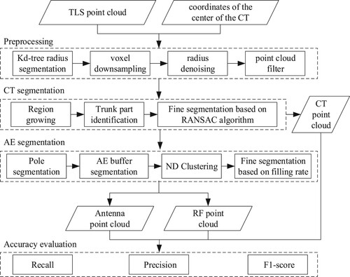
Figure 1 shows the technical flow diagram of the proposed method. The three main steps of segmenting the CT and AE point cloud are: 1) data preprocessing, 2) CT point cloud segmentation, 3) AE point cloud segmentation, and antenna and RFE point cloud classification. Details of each step are described in the following sections.

Figure 1 . Technical flow diagram of the proposed method.

2.1. Study area and dataset acquisition

The study area is in Guangxi Province, China. The main feature types in this area include CTs, roads, vegetation, and buildings. The scanning equipment is RIEGL vz-1000. The device’s Laser Beam Divergence is 0.3 mrad with a repeatability of 5 mm, the average point spacing of the collected data is 0.01 m, and the point density is 4000 pt/m².

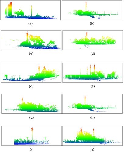
Ten data sets are selected containing typical CT types, named Data-I ∼ X, respectively, as shown in Figure 2. Data-I is a pipe tower, and there are four interference lamps on the upper part; Data-II is also a pipe tower, while there are no lamps or other interferences on the tower; Data-III is a triangular prism CT; Data-IV is a quadrangular CT; Data-V is also a pipe tower but compared with Data-I and Data-II, there are many connected holding poles between AE and the pole-shaped part; Data-VI is also a pipe tower. However, since AE is inside the safety cover, it is unnecessary to segment AE. Although Data-VII∼X are tube towers, the antennas and their corresponding RFE distributions are different to demonstrate the robustness of the AE segmentation algorithm for this variation.

Figure 2 . Dataset overview. (a)–(j) Data-I∼X, respectively.

Table 1 shows the area, number of points, number of CTs, number of antennas, and number of RFE in the test areas.

Table 1 . Statistics of dataset.

	Area (m^2)	Number of points	Number of CTs	Number of antennas	Number of RFE
Data-I	171 × 174	107 953 672	1	9	14
Data-II	147 × 166	42 615 143	1	9	5
Data-III	133 × 117	85 290 516	1	9	6
Data-IV	117 × 143	114 922 071	1	2	3
Data-V	160 × 152	61 941 588	1	5	5
Data-VI	146 × 147	74 337 912	1	0	0
Data-VII	149 × 174	42347656	1	9	12
Data-VIII	148 × 167	42657176	1	6	10
Data-IX	65 × 63	24326205	1	3	4
Data-X	160 × 152	64992213	1	12	7

2.2. Methodology

2.2.1 Preprocessing

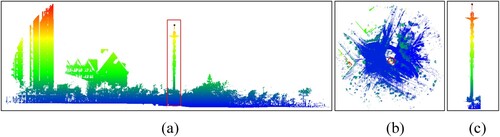
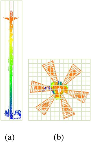
Preprocessing the input point cloud is necessary to remove noise and ground points and improve data processing efficiency. At first, Kd-tree segmentation method is utilized to segment the part of the point cloud containing the CT. This step manually extracts the coordinates of the center of the CT as the center of the circle and sets the segmentation radius r. The plane distance d between each point and the center is calculated, and the point cloud those corresponding d is smaller than r is kept (Figure 3), where r is set according to the cross-section dimensions of the CT.

Figure 3 . Schematic diagram of Kd-tree radius segmentation of the CT point cloud. (a) the front view, where the black point indicates the center point. (b) the top view. (c) the point cloud of CT obtained by Kd-tree radius segmentation.

Moreover, the voxel downsampling method (Shi and Rajkumar 2020) is utilized to uniform the point cloud density. Downsampling helps reduce randomness, improve the data operation efficiency, and handle large point cloud datasets. Then, point cloud denoising method based on connectivity analysis is adopted to remove the discrete noise points around the CT. This denoising method refers to traversing every point in the point cloud after downsampling. If each point has at least N neighboring points within a specific search radius R, the point will be retained; otherwise, it will be removed. Finally, an adaptive hierarchical threshold is utilized for the point cloud filter algorithm of moving surface fitting to remove the ground points (Zhu et al. 2018).

2.2.2 CT segmentation

The following steps are performed to segment the CT point cloud from the preprocessed point cloud: 1) Removing the miscellaneous points that are not connected with the CT using the region growing algorithm; 2) Identification of trunk part of the CT; 3) CT fine segmentation based on the RANSAC algorithm.

2.2.2.1. CT connectivity point segmentation

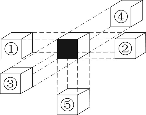
Since the CTs are often spaced from their surrounding vegetation, fences, and other features, there are usually empty grids on the tower and non-tower point grids at the same height. According to this feature, a five-neighborhood spatial grid region downward growing method is utilized based on the region growing idea to remove the grids that are not connected to the CT. The downward region growing method prevents stray spots below the tower from growing in again through the grid around the ground when the growth reaches the bottom of the communication tower. The steps of the algorithm are as follows.

1. Spatial grid division. Perform spatial grid division on the preprocessed point cloud. By setting the spatial grid size, including length l, width w, and height h, the point cloud is divided into a 3D grid according to the point cloud's x, y, and z coordinates.

2. Determination of the seed grid. Select the highest grid in the center of the CT as the seed grid and employ its number in the x, y, and z axes as the grid coordinates $\left(r_0,c_0,l_0\right)$.

3. The seed grid $\left(r_0,c_0,l_0\right)$ is utilized as the center. If the grid contains point cloud data in its five neighborhoods $\left(r_i,c_i,l_i\right)$ (front, back, left, right, and bottom, as shown in Figure 4), the number of points in the grid is compared with the threshold, and if it is greater than the threshold, the points in grids $\left(r_i,c_i,l_i\right)$ and $\left(r_0,c_0,l_0\right)$ are merged, and the grid coordinates are pressed into the stack.

4. Select the lowest grid $\left(r,c,l\right)$ in the stack, employ it as the seed grid in (2), and repeat step (3).

5. Repeat steps (3) to (4) until the stack is empty. Now, the point clouds in the connected grid are entirely extracted.

Figure 4 . five neighborhoods.

2.2.2.2. CT sub-part segmentation

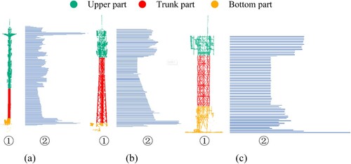
The CT can be divided into three parts: upper, trunk, and bottom. The trunk part refers to the smooth pole-shaped area, while the upper and bottom parts are placed above and bottom of the trunk part, respectively. Depending on the trunk part, the CT can be divided into three types: tube tower, triangular tower, and quadrangular tower, as shown in Figure 5①.

Figure. 5 . the CT structure and histogram of diagonal length and a layer height of each layer bounding box. (a) Tube tower. (b) Triangular tower. (c) Four-cornered tower. In each figure, ① indicates the CT structure, and ② indicates the histogram of diagonal length and layer height of each layer bounding box. The horizontal and vertical coordinates are the average length and height of the two diagonals. The reason for the lack of data at the top of the histogram is that there are fewer points at the top of the tower, and the resulting bounding box cannot be extracted.

(1) Trunk part identification

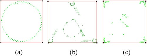
A vertical stratification strategy is utilized to identify the trunk part. First, the CT is divided into equally n layers at a certain interval $\mathrm{\Delta }h$ along with the z-axis, where $\mathrm{\Delta }h$ is set according to the total height of the CT, and the bounding box of the horizontal projection of each layer can be approximated as a quadrilateral, as indicated with the red box in Figure 6. The convex hull algorithm is employed to construct a contour polygon for each layer bounding box. The pipeline algorithm (Shen et al. 2008) is then utilized to simplify the contour polygon to detect the quadrilateral's corner points, as indicated with the black dots in Figure 6.

Figure 6 . Bounding box and corner points of the horizontal projection of a layer in the trunk part for three tower types. (a) Tube tower. (b) Triangular tower. (c) Four-cornered tower. The red line indicates the bounding box projection, and the black points indicate the corner points.

Then, the average length r of the two diagonals of the bounding box for each layer and the height h of the layer in which it is located are calculated. The variation of r with h is shown in the histogram in Figure 5 ②. As shown in Figure 5 ②, there is a linear relationship for the trunk part r and h (equation 1(1) $r=c_1\times h+c_0$(1) ) compared to an upper part with equipment or a bottom part with stray points attached. (1) $r=c_1\times h+c_0$(1) The trunk part is separated according to the linear relationship between r and h. In other words, the best linear model of r and h is established using the RANSAC algorithm. Then, the point cloud data of each layer conforming to the best linear model is extracted to completely identify the trunk part point cloud.

(2) Segmentation of upper and bottom parts

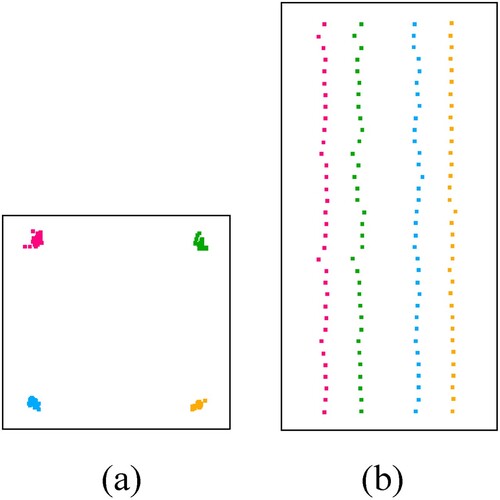
After the region grows, the bottom part of the CT is still closely connected with vegetation and other miscellaneous points. At the same time, there are no miscellaneous points around the upper and trunk parts. Thus, the upper and trunk parts are directly identified as the CT, and only the bottom part is processed. The corner points are partitioned into four subsets based on the orientation of each layer of the corner points located in the trunk part with respect to the center of the bounding box rectangle. Each subset can be approximately described with a three-dimensional straight line (Zhou et al. 2017), as shown in Figure 7(a). The corner points are fitted within the four subsets into four lines using the RANSAC algorithm, and the lines down to the tower’s bottom part are extracted to form the framework of the trunk and bottom parts, as shown in Figure 7(b). The point cloud is iterated at the bottom part; if the data points are inside the frame, they are kept; otherwise, they are recorded as miscellaneous points and are eliminated.

Figure 7 . Prismatic point diagram. (a) Top view. (b) Front view. Different colors indicate different prisms.

Finally, the point clouds of the upper, trunk, and bottom parts are merged to obtain the complete CT point cloud.

2.2.3. AE segmentation

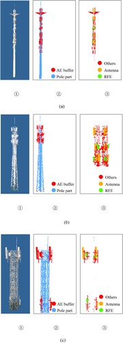
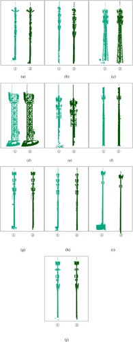
AE segmentation aims to obtain the point cloud of the antenna and RFE from the CT point cloud. The antenna and RFE on the CT have the following characteristics: 1) They do not intersect each other, 2) They are rectangular with a distinct plane surface, 3) They are significantly different in size. Therefore, considering the plane feature of the AE surface, the AE segmentation algorithm based on Normal Differential (ND) clustering is designed. The algorithm first segments the pole-shaped part point cloud and the AE buffer point cloud from the CT point cloud, as shown in Figure 8 ②. The antenna and RFE are further segmented and classified from the AE buffer point cloud, as shown in Figure 8 ③.

Figure 8 . CT with labels. (a) Tube tower. (b) Triangular tower. (c) Four-cornered tower. In each group, ① indicates the original CT point cloud displayed by RGB, ② indicates the AE buffer and pole-shaped part point cloud, and ③ indicates the AE and non-AE point cloud in the AE buffer.

2.2.3.1. Pole-shaped part segmentation

The purpose of pole-shaped part segmentation is twofold. The first is to improve computational efficiency. ND clustering calculates the normal vectors of K-nearest neighbors of a point. As the calculation is carried out point by point, the poles are removed first in order to prevent too many points from making the calculation too large. The second is to prevent the pole-shaped part from interfering with the AE segmentation due to the proximity of the normal vector. Pole-shaped part segmentation process includes 1) plane grid segmentation of the CT point cloud. This method is the division of each point into corresponding grids, based on the x and y coordinates of the point, at a certain grid size. As shown in Figure 9.

1. 2) growing all points in a single planar grid in the vertical space and judging whether there is a pole-shaped part point cloud in the plane grid according to the height of the point cloud growing (Wang et al. 2022). This is due to the good vertical connectivity of the pole-shaped part. The pole-shaped part should be connected in the vertical space after being divided by the plane grid. As the data integrity of TLS scanning decreases with the height increase, the point cloud with height increment becomes sparse. Therefore, under the assumption that the point cloud is always correctly oriented with the Z-axis facing upward, taking the point with the lowest z value in each plane grid as the seed point, the pole-shaped part is segmented using region upward growth of the spatial grid. The minimum z value is determined by traversing all the points in the planar grid, comparing the z value of each point, and selecting the minimum one.

Figure 9 . Plane grid segmentation. (a) Front view (b) Top view.

2.2.3.2 AE buffer segmentation

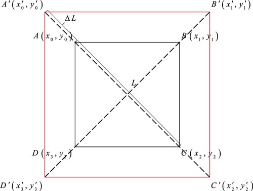
AE buffer refers to the point cloud containing AE after expanding the pole-shaped part outward for a certain distance. The pole-shaped part is extended outward as follows. The pole-shaped points are vertically layered at certain intervals along with the z-axis. Now, the four corner points of each layer of the bounding box are extracted, as described in section 2.2.2.

Taking the expanded corner point $C^{\mathrm{\prime }}$ as an example (as shown in Figure 10), the coordinates of $C^{\mathrm{\prime }}$ can be calculated from equations (2) to (6). Similarly, the coordinates of $A^{\mathrm{\prime }}$, $B^{\mathrm{\prime }}$, and $D^{\mathrm{\prime }}$can be obtained. (2) ${\displaystyle \frac{\overrightarrow{AC}}{\overrightarrow{C{C}^{\mathrm{\prime }}}}={\displaystyle \frac{L}{\mathrm{\Delta }L}}}$(2) (3) ${\displaystyle \frac{\left(x_2-x_0,y_2-y_0\right)}{\left({x^{\mathrm{\prime }}}_2-x_2,{y^{\mathrm{\prime }}}_2-y_2\right)}={\displaystyle \frac{L}{\mathrm{\Delta }L}}}$(3) (4) $\mathrm{\Delta }L\left(x_2-x_0,y_2-y_0\right)=L\left({x^{\mathrm{\prime }}}_2-x_2,{y^{\mathrm{\prime }}}_2-y_2\right)$(4) (5) $\{\begin{array}{c}\mathrm{\Delta }L\left(x_2-x_0\right)=L\left({x^{\mathrm{\prime }}}_2-x_2\right)\\ \mathrm{\Delta }L\left(y_2-y_0\right)=L\left({y^{\mathrm{\prime }}}_2-y_2\right)\end{array}$(5) (6) $\{\begin{array}{c}{x^{\mathrm{\prime }}}_2=x_2+\left(x_2-x_0\right)\times \mathrm{\Delta }L/L\\ {y^{\mathrm{\prime }}}_2=y_2+\left(y_2-y_0\right)\times \mathrm{\Delta }L/L\end{array}$(6) where $\mathrm{\Delta }L$ is the extended distance along with diagonal $\left(x_2-x_0,y_2-y_0\right)$; $\left({x^{\mathrm{\prime }}}_2,{y^{\mathrm{\prime }}}_2\right)$ indicates the coordinates of the expanded corner point C; $\left(x_0,y_0\right)$ and $\left(x_2,y_2\right)$ are the coordinates of corner points A and C, respectively, and L is the diagonal length of the bounding box.

Figure 10 . The original and expanded corner points of the bounding box. A, B, C, and D indicate the original corner points, and $A^{\mathrm{\prime }}$, $B^{\mathrm{\prime }}$, $C^{\mathrm{\prime }}$ and $D^{\mathrm{\prime }}$ indicate the expanded corner points.

If any CT point P is inside the expanded bounding box, it is a non-AE buffer point; otherwise, it is an AE buffer point. In order to determine whether a point is in the expanded bounding box of the corresponding layer, the inequalities (7) should be satisfied. (7) $\{\begin{array}{c}\left(\overrightarrow{P{A}^{\mathrm{\prime }}}\times \overrightarrow{P{B}^{\mathrm{\prime }}}\right)\cdot \left(\overrightarrow{P{D}^{\mathrm{\prime }}}\times \overrightarrow{P{C}^{\mathrm{\prime }}}\right)\le 0\\ \left(\overrightarrow{P{B}^{\mathrm{\prime }}}\times \overrightarrow{P{C}^{\mathrm{\prime }}}\right)\cdot \left(\overrightarrow{P{A}^{\mathrm{\prime }}}\times \overrightarrow{P{D}^{\mathrm{\prime }}}\right)\le 0\end{array}$(7) where point P is the point cloud data to be judged, $A^{\mathrm{\prime }}$, $B^{\mathrm{\prime }}$, $C^{\mathrm{\prime }}$and $D^{\mathrm{\prime }}$ are expended corner points.

2.2.3.3. Fine segmentation and classification of AE

The process of segmenting and classifying AE is as follows. ND Clustering is applied to cluster the AE buffer point cloud with the same normal vector values. The plane of each cluster is extracted, and the plane’s point cloud filling rate is calculated to segment the clusters containing AE. Besides, the AE is labeled as antenna or RFE through the a priori size information of antenna and RFE, respectively.

(1) ND clustering

ND clustering is employed to cluster the point cloud in the AE buffer. For each point p of the input point cloud P, the method employs two different kd-tree neighborhood point thresholds to estimate two normal vectors for the same point. The ND feature is defined according to the difference of the unit normal vector of the input point cloud, as shown in equation (8)(8) $\mathrm{\Delta }n\left(p,n_1,c_2\right)={\displaystyle \frac{n\left(p,c_1\right)-n\left(p,c_2\right)}{2}}$(8) . The point cloud corresponding to the target scale is segmented by setting the ND threshold. Finally, the points with similar ND values are classified into the same cluster based on the Euclidean clustering: (8) $\mathrm{\Delta }n\left(p,n_1,c_2\right)={\displaystyle \frac{n\left(p,c_1\right)-n\left(p,c_2\right)}{2}}$(8) where$n\left(p,c_1\right)$ and $n\left(p,c_2\right)$ are the estimated values of the normal surface vector of point p when the number of points is denoted by $c_1$ and $c_2$ ($c_1$<$c_2$). After repeated trials, $c_1$and $c_2$ are set to 8 and 16, respectively.

(2) Calculation of point cloud filling rate

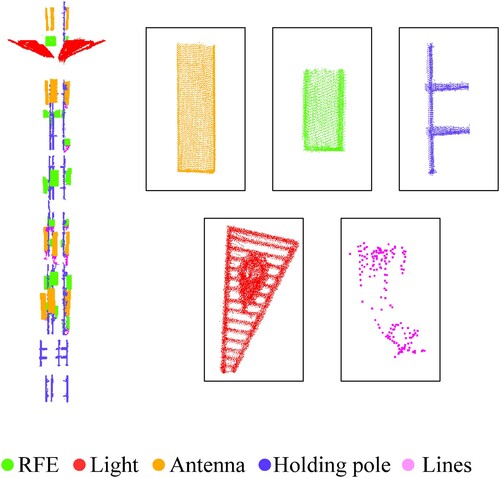
The clusters obtained by ND clustering include antennas, RFE, lines, holding poles, and other objects. RFE and antennas have a rectangular shape and distinctive regular quadrilateral planar features on their outer surface. The line features of the holding bar and line are significant. The light is an irregular trilateral shape, as shown in Figure 11. While extracting the plane of each cluster, the plane points extracted from RFE and antenna should fill the whole quadrilateral, while the plane points extracted from lines, holding poles, and other objects cannot fill the whole quadrilateral. Therefore, the point cloud filling rate of the plane is calculated by extracting the plane of each cluster, and the cluster less than the filling rate threshold is removed to obtain accurate AE points.

Figure 11 . Buffer equipment.

The calculation steps of the plane’s point cloud filling rate are as follows: 1) Extracting the plane from each class cluster; 2) Removing outliers around the plane; 3) Rotating the plane point cloud to the principal direction by Principal Component Analysis (PCA); 4) Extracting the plane grid in the previous step with a specific grid size and calculating the number of filled grids at the existing points and the total number of grids contained in the plane’s external rectangle. The size of the grid in the x-direction and z-direction is one-tenth of the length of the plane in these two directions, respectively. Then, the plane’s point cloud filling rate can be described by (9): (9) $f={\displaystyle \frac{gnp}{gn}}$(9) where $f$ is the filling rate of the point cloud, gnp is the number of grids with points, and gn is the total number of grids contained in the plane’s circumscribed rectangle.

The length and height of the plane are calculated after Principal Component Analysis (PCA) redirect and are compared with the a priori values of the length and height of RFE and antenna to judge whether this cluster is an antenna point, RFE point, or other types. As we are calculating the dimensions of the plane profile of the AE, we need to ensure that the points of the plane profile are complete and that the absence of the point inside the plane does not affect the effect of the dimensioning.

The point cloud used in the segmentation of the CT and AE has been downsampled. These points represent centroid in each voxel grid. Finally, the original points in the voxel grid should be indicated in the same category as the voxel grid's centroid.

2.2.4. Accuracy evaluation

Point-based and object-based strategies are utilized to quantitatively evaluate the algorithm's performance in CT, antenna, and RFE segmentation. The point clouds for CTs and AE are manually labelled as the ground truth values.

(1) Point-based strategy

In order to perform the Point-by-point comparison of the target points segmented by the algorithm with the ground truth values, Recall, Precision, and F1-score (Singh, Raval, and Banerjee 2021), are adopted as evaluation indices. The Recall represents the percentage of correctly detected target objects in the actual value, Precision represents the percentage of correctly detected target objects in all detection results, and the F1-score is the harmonic average of Recall and Precision. The calculation method is shown in (10) ∼ (12): (10) $Recall={\displaystyle \frac{TP}{TP+FN}}$(10) (11) $Precision={\displaystyle \frac{TP}{TP+FP}}$(11) (12) $F1=2\times {\displaystyle \frac{Recall\times Precision}{Recall+Precision}}$(12) where TP, FN, and FP represent the number of target object points that are correctly detected, undetected, and incorrectly detected in the result, respectively.

(2) Object-based strategy

Object-based strategy compares the number of AE segmented by the algorithm with the ground truth (manually segmented objects). If more than 95% of the points in a single AE are correctly identified, the AE object is correctly segmented. Although Recall, Precision, and F1-score are also employed as the evaluation indices, their meaning differ from that of the point-based evaluation. Recall indicates the percentage of correctly detected device objects in the ground truth, and Precision indicates the percentage of correctly detected device objects in all detection results. TP, FN, and FP indicate the number of correctly detected, undetected, and incorrectly detected objects, respectively.

3. Experimentation and analysis

In order to evaluate the effectiveness and robustness of the proposed method, 10 data sets are tested. The experimental results are analyzed from three aspects: (1) the result figures of CT preprocessing and segmentation, (2) the result figures of antenna and RFE segmentation, (3) quantitative analysis of the segmentation accuracy of CTs, antennas and RFE using point-based and object-based strategies. The programming language is C + +, implemented on a Dell desktop, Intel (R) Core (TM) i7-10700 CPU @ 2. 90ghz with 24.0 GB RAM.

3.1. CT segmentation results

For the CT segmentation algorithm proposed in Section 2.2, this section experimentally analyzes the point cloud data of each CT with different structures. The main parameters are set as follows: (1) The downsampled voxel grid size is set to 0.05 m because the average spacing of the point clouds is 0.01 m. (2) The grid's length, width, and height are set to 0.5 m during the spatial grid region growth because the noise removal effect is not evident for larger values of the grid size. In general, the grid size is 5–10 times the average point spacing. If it is less than this interval, it results in more empty meshes (without any point cloud data). (3) The vertical stratification interval in the trunk part identification is set to 0.05 m. The too-large interval will lead to the lack of a fine relationship between the diagonal and the height of the bounding box in each layer. In contrast, a too-small interval may lead to a long calculation time for each layer. Figure 12 shows CTs’ preprocessing and segmentation results in Data-I to Data-X. Compared with the original dataset in Figure 2, the CT segmentation algorithm can effectively segment the CT point cloud.

Figure 12 . Preprocessing and segmentation results of CTs. (a)∼(j) are Data-I∼X, respectively. where ① in each figure indicates the preprocessing result and ② indicates the CT segmentation result.

3.2. AE segmentation results

Precise segmentation of antennas and RFE is performed on each CT. The main parameters are set as follows. 1) The length and width of the planar grid are set to 0.2 m when the pole-shaped part is segmented, considering the small planar projection area of the pole-shaped part. The length, width, and height of the spatial grid region growing upward are set to 1 m. 2) When segmenting the AE buffer, the corner’s outward expansion distance depends on the distance from the AE to the pole-shaped part. Since the AE in Data-I, Data-II, and Data-IV are closely connected with the pole-shaped part, the distance is set to 0.02 m. There is a holding pole between the AE and the pole-shaped part in Data-III and Data-V, resulting in a large spacing between the two parts. Thus, the distance can be appropriately expanded to 0.4 m. In general, the parameter value should be less than 0.4. 3) In ND-based clustering, the distance threshold between point and plane is set to 0.2 m, considering that the edges of the antenna and RFE will have a small normal differential. 4) During the fine segmentation of AE, considering that the collected AE point cloud will be missing, the plane of AE extracted from the cluster may be incomplete due to blindspots. Therefore, after repeated experiments, the plane’s point cloud filling rate is set to 70%. 5) In order to further separate antenna and RFE points from the obtained AE point cloud, the size thresholds of antenna and RFE are determined according to their design specifications, as shown in Table 2.

Table 2 . The empirical size thresholds of antenna and RFE.

	Height (m)	Length(m)	Thickness (m)
Antenna	1–2	0.2–0.4	0.15–0.2
RFE	0.3–0.5	0.3–0.4	0.15–0.2

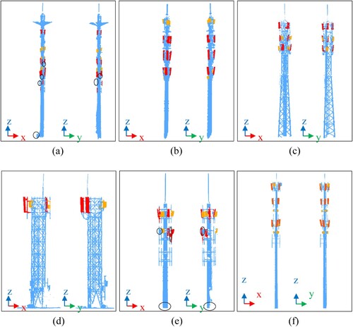
Figure 13 shows the segmentation results of AE, in which the red and yellow points indicate the antenna and the RFE points, respectively. The AE in data VI is enclosed in the safety cover and cannot be divided. The results show that the proposed AE segmentation algorithm is free from the interference of lamps and other sundries on the CT and independent of the type of CTs and the distribution of AE. It can accurately segment the antenna and RFE points and has strong adaptability and robustness.

Figure 13. Segmentation results of CTs and AE: (a) ∼(i) are Data-I∼IX. All points in this Figure are CT points. Among them, the red point is the antenna point, the yellow point is the RFE point, and the point in the black circle is the wrong or omitted point.

3.3. Accuracy evaluation

Point-based and object-based strategies are employed to quantify the segmentation accuracy of CTs, antennas, and RFE. Table 3 shows the point-based accuracy of point cloud segmentation of CTs and AE. The average Recall, Precision, and F1-score of CTs are 97. 52%, 99. 92%, and 98. 70%, respectively. The corresponding values for antennas are 97. 91%, 94. 51% and 96. 09%, respectively. The corresponding values for RFE are 86. 31%, 94. 38% and 89. 89%, respectively.

Table 3 . Point-based segmentation accuracy of CTs and AE.

	Type	Real value	TP	FP	FN	Recall (%)	Precision (%)	F1 (%)
Data-I	CT	726876	693117	1650	33759	95. 36	99. 76	97. 51
	Antenna	56831	55582	11918	1249	97. 8	82. 34	89. 41
	RFE	31406	28738	342	2668	91. 5	98. 82	95. 02
Data-II	CT	238208	237902	4	306	99. 87	100	99. 93
	Antenna	59120	57053	1819	2067	96. 5	96. 91	96. 71
	RFE	14876	13124	323	1752	88. 22	97. 6	92. 67
Data-III	CT	3303476	3239742	22	63734	98. 07	100	99. 03
	Antenna	86801	86426	8177	375	99. 57	91. 36	95. 29
	RFE	55553	54615	5526	938	98. 31	90. 81	94. 41
Data-IV	CT	3625714	3557604	11624	68110	98. 12	99. 67	98. 89
	Antenna	74011	73798	5264	213	99. 71	93. 34	96. 42
	RFE	29682	26197	3994	3485	88. 26	86. 77	87. 51
Data-V	CT	187610	177572	2	10038	94. 65	100	97. 25
	Antenna	25689	25542	2166	147	99. 43	92. 18	95. 67
	RFE	24082	20546	1159	3536	85. 32	94. 66	89. 75
Data-VI	CT	3114598	3114214	434	384	99. 99	99. 99	99. 99
Data-VII	CT	357545	347882	122	9663	97. 30	99. 96	98. 61
	Antenna	33318	32910	250	408	98. 78	99. 25	99. 01
	RFE	15309	13030	571	2279	85. 11	95. 80	90. 14
Data-VIII	CT	396898	378293	37	18605	95. 31	99. 99	97. 60
	Antenna	32761	32342	260	419	98. 72	99. 20	98. 96
	RFE	17227	15843	393	1384	91. 97	97. 58	94. 69
Data-IX	CT	294568	288698	74	5870	98. 01	99. 97	98. 98
	Antenna	15123	14465	59	658	95. 65	99. 59	97. 58
	RFE	7472	6367	205	1105	85. 21	96. 88	90. 67
Data-X	CT	414753	408779	566	5974	98. 56	99. 86	99. 21
	Antenna	57062	54223	2012	2839	95. 02	96. 42	95. 72
	RFE	9229	5802	612	3427	62. 87	90. 46	74. 18

The object-based segmentation results are shown in Table 4. The average Recall, Precision, and F1-score of antennas are 99. 07%, 97. 22% and 97. 93%, respectively. The corresponding values for RFE are 82. 91%, 100. 00% and 90. 00%, respectively. The accuracy indicates a good segmentation effect of the proposed method.

Table 4 . Object-based segmentation results for antennas and RFE.

	Type	TP	FP	FN	Recall (%)	Precision (%)	F1 (%)
Dataset-I	Antenna	9	3	0	100. 00	75. 00	85. 71
	RFE	12	0	2	85. 71	100. 00	92. 31
Dataset-II	Antenna	9	0	0	100. 00	100. 00	100. 00
	RFE	5	0	0	100. 00	100. 00	100. 00
Dataset-III	Antenna	9	0	0	100. 00	100. 00	100. 00
	RFE	6	0	0	100. 00	100. 00	100. 00
Dataset-IV	Antenna	2	0	0	100. 00	100. 00	100. 00
	RFE	2	0	1	66. 67	100. 00	80. 00
Dataset-V	Antenna	5	0	0	100. 00	100. 00	100. 00
	RFE	4	0	1	80. 00	100. 00	88. 89
Data-VII	Antenna	9	0	0	100. 00	100. 00	100. 00
	RFE	11	0	1	91. 67	100. 00	95. 65
Data-VIII	Antenna	6	0	0	100. 00	100. 00	100. 00
	RFE	9	0	1	90. 00	100. 00	94. 74
Data-IX	Antenna	3	0	0	100. 00	100. 00	100. 00
	RFE	3	0	1	75. 00	100. 00	85. 71
Data-X	Antenna	11	0	1	91. 67	100. 00	95. 65
	RFE	4	0	3	57. 14	100. 00	72. 73

Further analysis indicates that when the antenna and RFE are closely connected, and the gap is small, the ND clustering algorithm will classify the two into one class due to the similarity of the two normal vectors, leading to misclassification of the AE. Nevertheless, this algorithm can still effectively segment most CT and AE points, while the average values of Recall, Precision, and F1-score are more than 90%.

4. Discussion

In order to investigate the impact of the algorithm parameters on the F1-score, two main parameters affecting the segmentation accuracy of AE are analyzed. Data-I is employed as an example for sensitivity analysis because the same set of algorithms is used for data preprocessing, CT point cloud segmentation, antenna and RFE point cloud segmentation, and classification for the communication base station data covered in the paper. The sensitivity analysis adopts the control variable method. Accordingly, each experiment only changes the value of its corresponding test parameters and sets the values of other parameters as the default values.

4.1. Outward expansion distance of corners

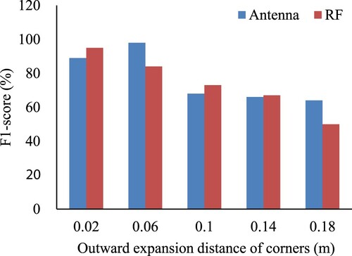
The distance from the corner to the outside influences the AE buffer’s segmentation. The distances are set as 0. 02 m, 0. 06 m, 0. 1 m, 0. 14 m, and 0. 18 m and their corresponding F1-score values are shown in Figure 14. In Data-I, the AE is close to the tower. If the distance is too large, part of the longitudinal section of the AE will not be in the buffer zone, missing the AE point cloud in the buffer zone. Therefore, the Recall will be reduced when segmenting the point cloud in the AE buffer due to the incomplete AE point cloud. The greater the distance, the lower the accuracy. In this paper, the distance of Data-I is set to a smaller value of 0. 02 m.

Figure 14 . F1-score values of the outward expansion distance of different corners.

4.2. Distance from point to plane

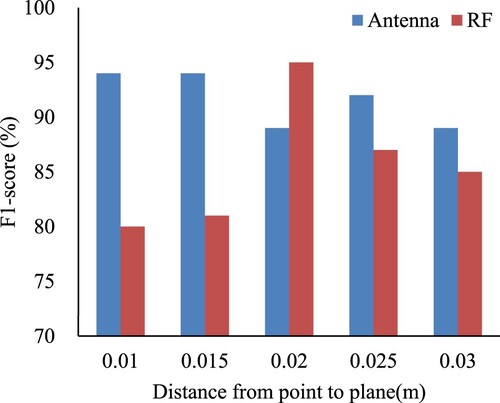
The distance from the point to the plane affects the plane extraction accuracy. The corresponding F1-score values for the distances 0. 01 m, 0. 015 m, 0. 02 m, 0. 025 m, and 0. 03 m are shown in Figure 15. The outer plane of AE is usually not a standard plane but has a radian. Thus, if this value is small, the points at both ends of the arc may be regarded as non-AE points because they do not meet the distance threshold from point to plane, reducing Recall; otherwise, the AE line point cloud cluster may be wrongly divided into AE point cloud because the lines are arranged neatly, reducing the Precision. In order to achieve a high-accuracy antenna and RFE, this value is set to 0. 02 m in this paper.

Figure 15 . F1-score values corresponding to the distance from different points to plane.

5. Conclusion

Obtaining accurate measurement data of CTs helps calculate the tilt angle and settlement of CTs accurately and timely discover the deformation and tilt of CTs. It also helps clarify the location and quantity of existing AE on the CT, providing a planning basis for the reasonable layout of AE. The point cloud of the CT and AE contains information like location and geometry, which provides primary data for the intelligent management and maintenance of the communication base station. However, the point cloud should be segmented in advance to model the CT together with AE and further calculate their inclinations. Limited research has been performed on the fine segmentation of communication base station scene objects. Therefore, this paper proposes a segmentation method of CT and AE point cloud based on geometric features, which is suitable for various tower types, including CT point cloud segmentation based on region growing and RANSAC algorithm, AE point cloud segmentation based on pole-shaped partial segmentation, ND clustering and point cloud filling rate, and antenna and RFE points classification according to a priori size of AE. The experimental results demonstrate that the average values of Recall, Precision, and F1-score of CTs and AE point cloud are all above 90%. It demonstrates that the proposed method is robust to the segmentation of various types of CTs and AE and can be applied to different types of CTs.

The advantages and characteristics of the proposed method are mainly reflected in the following aspects:

1. The region growing and RANSAC algorithms can effectively eliminate miscellaneous points such as vegetation and fences around the CT when the CT is segmented. In addition, as long as the geometry of the CT does not change, even if the CT is tilted or inclined at a certain angle, the CT points can still be segmented using the CT segmentation algorithm in this paper.

2. By analyzing the AE’s planar features, ND clustering can effectively cluster the point clouds with smaller differences in normal vector values into one class.

3. The proposed point cloud fill rate can effectively distinguish objects such as lights, holding poles, and lines on the CT that also have the characteristic of small differences in normal vector values from AE.

4. Compared with machine learning methods, the proposed algorithm does not require much training data, does not require high memory for computer operations, and is not influenced by sample imbalance. It can accurately segment different scenes of CTs and AE and has strong robustness.

Although the proposed method achieves high accuracy and Recall for the segmentation of CT and AE point clouds, it is challenging to evaluate the segmentation accuracy of deep neural networks for CTs and AE due to the lack of sufficient training data. Besides, only the segmentation accuracies of the TLS point cloud-based CTs and AE are evaluated due to the limitation of the acquisition devices. Future work could further explore geometric features of the target objects to improve the method's adaptability. As more datasets become available through a number of 3D imaging devices, such as mobile/airborne LiDAR or photogrammetry, deep neural networks may be employed for classification at a larger scale and in a more complex environment.

Acknowledgements

We thank the anonymous reviewers for their constructive comments on this manuscript.

Disclosure statement

No potential conflict of interest was reported by the author(s).

Additional information

Funding

This research was funded by Guangxi Natural Science Fund for Innovation Research Team [grant number 2019GXNSFGA245001]; High-Level Talent Aggregation Project in Hunan Province, China-Innovation Team [grant number 2019RS1060].

References

- Ali, Marwah T, Yousif R Muhsen, Raad Farhood Chisab, and Sameeha N Abed. 2021. “Evaluation Study of Radio Frequency Radiation Effects from Cell Phone Towers on Human Health.” Radioelectronics and Communications Systems 64 (3): 155–164. doi:10.3103/S0735272721030055
- Burd, Paul Ray, Karl Mannheim, Tobias März, Jonas Ringholz, Alexander Kappes, and Matthias Kadler. 2018. “Detecting Radio Frequency Interference in Radio-Antenna Arrays with the Recurrent Neural Network Algorithm.” Astronomische Nachrichten 339 (5): 358–362. doi:10.1002/asna.201813505
- Chen, Shichao. 2020. Study on High-Voltage Transmission Line Reconstruction Based on Airborne LiDAR Point Cloud. Beijing: China University of Mining & Technology.
- Fu, Shu, Jie Gao, and Lian Zhao. 2020. “Integrated Resource Management for Terrestrial-Satellite Systems.” IEEE Transactions on Vehicular Technology 69 (3): 3256–3266. doi:10.1109/TVT.2020.2964659
- Gao, Jie, Lian Zhao, and Xuemin Shen. 2019. Service Offloading in Terrestrial-Satellite Systems: User Preference and Network Utility. Paper Presented at the 2019 IEEE Global Communications Conference (GLOBECOM).
- Huo, Yiming, Xiaodai Dong, and Scott Beatty. 2020. “Cellular Communications in Ocean Waves for Maritime Internet of Things.” IEEE Internet of Things Journal 7 (10): 9965–9979. doi:10.1109/JIOT.2020.2988634
- Huo, Yiming, Franklin Lu, Felix Wu, and Xiaodai Dong. 2019. Multi-Beam Multi-Stream Communications for 5G and Beyond Mobile User Equipment and UAV Proof of Concept Designs. Paper Presented at the 2019 IEEE 90th Vehicular Technology Conference (VTC2019-Fall).
- Lukacs, Mathew W, Angela J Zeqolari, Peter J Collins, and Michael A Temple. 2015. ““RF-DNA” Fingerprinting for Antenna Classification.” IEEE Antennas and Wireless Propagation Letters 14: 1455–1458. doi:10.1109/LAWP.2015.2411608
- Meng, T. 2018. “Research on the Adjustment Work of Transmission Line Poles.” J. Electric Engineering 3: 122–123.
- Motlagh, Naser Hossein, Tarik Taleb, and Osama Arouk. 2016. “Low-altitude Unmanned Aerial Vehicles-Based Internet of Things Services: Comprehensive Survey and Future Perspectives.” IEEE Internet of Things Journal 3 (6): 899–922. doi:10.1109/JIOT.2016.2612119
- Nowak, Rafał, Romuald Orłowicz, and Radosław Rutkowski. 2020. “Use of TLS (LiDAR) for Building Diagnostics with the Example of a Historic Building in Karlino.” Buildings 10 (2): 24. doi:10.3390/buildings10020024
- Pahlavan, Kaveh, Julang Ying, Ziheng Li, Erin Solovey, John Patrick Loftus, and Zehua Dong. 2020. “RF Cloud for Cyberspace Intelligence.” IEEE Access 8: 89976–89987. doi:10.1109/ACCESS.2020.2993548
- Shen, Wei, Jing Li, Y. H. Chen, Lei Deng, and G. X. Peng. 2008. “Algorithms Study of Building Boundary Extraction and Normalization Based on Lidar Data.” Journal of Remote Sensing 12 (5): 692–698.
- Shi, Weijing, and Raj Rajkumar. 2020. Point-gnn: Graph Neural Network for 3d Object Detection in a Point Cloud. Paper Presented at the Proceedings of the IEEE/CVF Conference on Computer Vision and Pattern Recognition.
- Singh, Sarvesh Kumar, Simit Raval, and Bikram Banerjee. 2021. “A Robust Approach to Identify Roof Bolts in 3D Point Cloud Data Captured from a Mobile Laser Scanner.” International Journal of Mining Science and Technology 31 (2): 303–312. doi:10.1016/j.ijmst.2021.01.001
- Tan, Hongwu, Jingru Wang, Wuneng Liu, Lilong Liu, and Xiaohuan Xi. 2021. “Automatic Extraction of High Voltage Line Tower Point Cloud from Airborne LiDAR Data.” Remote Sensing Information 4.
- Tan, Junxiang, Haojie Zhao, Ronghao Yang, Hua Liu, Shaoda Li, and Jianfei Liu. 2021. “An Entropy-Weighting Method for Efficient Power-Line Feature Evaluation and Extraction from LiDAR Point Clouds.” Remote Sensing 13 (17): 3446. doi:10.3390/rs13173446
- Wang, S. L., Y. Du, J. X. Sun, Q. Fang, Y. C. Weng, L. Ma, X. F. Zhang, J. Wu, Q. Qin, and Q. S. Shi. 2018. “Effect of Superficial gas Velocity on Solid Behaviors in a Full-Loop CFB.” Powder Technology 333: 91–92. doi:10.1016/j.powtec.2018.04.011
- Wang, Jingru, Cheng Wang, Xiaohuan Xi, Pu Wang, Meng Du, and Sheng Nie. 2022. “Location and Extraction of Telegraph Poles from Image Matching-Based Point Clouds.” Remote Sensing 14 (3): 433. doi:10.3390/rs14030433
- Zhang, Ruizhuo, Bisheng Yang, Wen Xiao, Fuxun Liang, Yang Liu, and Ziming Wang. 2019. “Automatic Extraction of High-Voltage Power Transmission Objects from UAV Lidar Point Clouds.” Remote Sensing 11 (22): 2600. doi:10.3390/rs11222600
- Zhang, Guangxin, Liying Zhao, Dongliang Qiao, Ziwen Shang, and Rui Huang. 2021. Design of Transmission Line Safety Early Warning System Based on Big Data Variable Analysis. Paper Presented at The 2021 International Conference on Intelligent Transportation, Big Data & Smart City (ICITBS).
- Zhao, Jian, Di Wang, Xin Long, Shaohua Wu, and Wei Hu. 2020. Power Tower Extraction Method Under Complex Terrain in Mountainous Area Based on Laser Point Cloud Data. Paper Presented at the IOP Conference Series: Earth and Environmental Science.
- Zhou, Ruqin, Wanshou Jiang, Wei Huang, Bo Xu, and San Jiang. 2017. “A Heuristic Method for Power Pylon Reconstruction from Airborne LiDAR Data.” Remote Sensing 9 (11): 1172. doi:10.3390/rs9111172
- Zhou, M., K. Y. Li, J. H. Wang, C. R. Li, G. E. Teng, L. Ma, H. H. Wu, W. Li, H. J. Zhang, and J. Y. Chen. 2019. “Automatic Extraction of Power Lines from UAV Lidar Point Clouds Using a Novel Spatial Feature.” ISPRS Annals of the Photogrammetry, Remote Sensing and Spatial Information Sciences IV-2/W7: 227–234. doi:10.5194/isprs-annals-IV-2-W7-227-2019
- Zhu, Xiaoxiao, Cheng Wang, Xiaohuan Xi, Pu Wang, Xinguang Tian, and Xuebo Yang. 2018. “Hierarchical Threshold Adaptive for Point Cloud Filter Algorithm of Moving Surface Fitting.” Acta Geodaetica et Cartographica Sinica 2: 153–160.