Evaluation of nine machine learning methods for estimating daily land surface radiation budget from MODIS satellite data

ABSTRACT

The all-wave net radiation (Rn) at the land surface represents surface radiation budget and plays an important role in the Earth's energy and water cycles. Many studies have been conducted to estimate from satellite top-of-atmosphere (TOA) data using various methods, particularly the application of machine learning (ML) and deep learning (DL). However, few studies have been conducted to provide a comprehensive evaluation about various ML and DL methods in retrieving. Based on extensive in situ measurements distributed at mid-low latitudes, the corresponding Moderate Resolution Imaging Spectroradiometer (MODIS) TOA observations, and the daily from the fifth generation of European Centre for Medium-Range Weather Forecasts Reanalysis 5 (ERA5) used as a priori knowledge, this study assessed nine models for daily estimation, including six classic ML methods (random forest -RF, adaptive boosting - Adaboost, extreme gradient boosting -XGBoost, multilayer perceptron -MLP, radial basis function neural network -RBF, and support vector machine -SVM) and three DL methods (multilayer perceptron neural network with stacked autoencoders -SAE, deep belief network -DBN and residual neural network -ResNet). The validation results showed that the three DL methods were generally better than the six ML methods except XGBoost, although they all performed poorly in certain conditions such as winter days, rugged terrain, and high elevation. ResNet had the most robust performance across different land cover types, elevations, seasons, and latitude zones, but it has disadvantages in practice because of its highly configurable implementation environment and low computational efficiency. The estimated daily values from all nine models were more accurate than the corresponding Global LAnd Surface Satellite (GLASS) product.

KEYWORDS:

• Net radiation
• energy balance
• mid-low latitude
• model comparison
• machine learning
• deep learning
• MODIS
• ERA5

1. Introduction

Surface all-wave net radiation ($R_n$), which characterizes the available radiative energy budget at the Earth’s surface, drives most biological and physical processes, such as heating the soil and air, evapotranspiration (ET), photosynthesis and so on (Jiang et al. 2014). Therefore, $R_n$ plays an essential role in energy redistribution and the global hydrological and carbon cycle (Alados et al. 2003; Verma et al. 2016). $R_n$ is mathematically expressed as the difference between the surface incoming and outgoing shortwave and longwave radiation (Bisht et al. 2005): (1) $R_n=R_{ns}+R_{nl}$(1) (1a) $R_{ns}=R_s^{\downarrow }-R_s^{\uparrow }=\left(1-\alpha \right)R_s^{\downarrow }$(1a) (1b) $R_{nl}=R_l^{\downarrow }-R_l^{\uparrow }$(1b) where $R_{ns}$ and $R_{nl}$ are the surface net shortwave radiation (Wm⁻², downwards is defined as positive) and net longwave radiation (Wm⁻²), respectively; $R_s^{\downarrow }$, $R_s^{\uparrow }$,$R_l^{\downarrow }$, and $R_l^{\uparrow }$ are the surface downwards shortwave radiation (Wm⁻²), upwards shortwave radiation (Wm⁻²), downwards longwave radiation (Wm⁻²) and upwards longwave radiation (Wm⁻²), respectively; $\alpha$ is the surface shortwave broadband albedo; and $R_s^{\uparrow }$ is calculated by $\alpha \times R_s^{\downarrow }$.

$R_n$ or its four radiative components could be directly measured at the site, but these measurements only determine the $R_n$ at individual points (da Silva et al. 2015) and are sparsely distributed (Bisht and Bras 2010; Chen et al. 2020; Xu, Liang, and Jiang 2022). Hence, because of the unique advantages such as spatiotemporal continuous and global coverage, satellite data is widely used to generated $R_n$ products ranging from regional to global scales, especially the data from Moderate Resolution Imaging Spectroradiometer (MODIS), which onboard the Terra and Aqua satellites (Bisht et al. 2005; Wang et al. 2015a). Generally, the algorithms for estimating the $R_n$ from satellite observations can be roughly divided into two categories (Liang et al. 2010): one calculates radiative quantities from the high-level satellite products of related surface or atmospheric variables (e.g. aerosols, clouds, and atmospheric temperature and humidity profiles) (Carmona, Rivas, and Caselles 2015; Verma et al. 2016), and the other estimates radiation directly from satellite top-of-atmosphere (TOA) observations (called a satellite TOA data-driven algorithm), in which the extensive radiation either simulating from the radiative transfer models (Kim and Liang 2010; Wang et al. 2015b) or collecting from comprehensive ground measurements (Chen et al. 2020; Li et al. 2021) were linked with various statistical models without taking the complicated physical mechanism of an atmospheric radiative transmission into account. The format of the second type of algorithm is simple, and its inputs are easily obtained; hence, it has become increasingly popular in recent years. Wang et al. (2015a) proposed a MODIS TOA data-driven algorithm to estimate $R_n$ based on simulations from MODTRAN5, and the results were validated to achieve higher accuracy than that of other component-based method. However, aware of the limitations in the model simulations and linear statistical method, Chen et al. (2020) developed a new model to estimate the all-sky daily $R_n$ from the MODIS TOA observations at high latitudes according to a similar framework but based on the ground measurements and with a novel artificial neural network tuned by a genetic algorithm. Afterwards, Li et al. (2021) applied a similar idea to estimate the $R_n$ at a relatively high spatial resolution (1 km) at mid-low latitudes from MODIS TOA data by using the random forest (RF) method. In addition, the authors introduced the daily $R_n$ from the fifth generation of the European Center for Medium-Range Weather Forecasts Reanalysis 5 (ERA5) (Hersbach et al. 2020) reanalysis data as a priori knowledge to address the issue of few information provided by the available MODIS TOA observation in this study. The validation results were satisfactory and superior to three existing good performing $R_n$ products, including the MODIS $R_n$ product from the Global LAnd Surface Satellite (GLASS) products suite (referred to as GLASS-MODIS hereinafter) (Liang et al. 2021), the Edition 4A of Synoptic TOA and surface fluxes and clouds from the Clouds and the Earth’s Radiant Energy System (CERES SYN1deg_Ed4A), referred to as CERES4A hereinafter (Kratz et al. 2020) and FLUXCOM_RS. Similarly, (Xu, Liang, and Jiang 2022) generated a global $R_n$ product from 1981 to 2019 based on Advanced Very High Resolution (AVHRR) TOA observations but using a deep learning (DL) method named the residual convolutional neural network (RCNN); the authors concluded that this method performed better than the $R_n$ from second generation of Modern-Era Retrospective Analysis for Research and Applications (MERRA2), GLASS-MODIS, and CERES4A. Therefore, these studies indicate that the advantages of the satellite TOA data-driven algorithm in $R_n$ estimation is outstanding but the performance of this kind of algorithm highly depends on the representativeness and comprehensiveness of the samples used for modeling and the regression abilities of the statistical method, whose influences on algorithm performance were less discussed comparing to samples.

With the development of data-driven methods, an increasing number of ML methods, especially DL methods, including the convolutional neural network (CNN), deep belief network (DBN) (Hinton, Osindero, and Teh 2006), tacked automatic encoding machine (SAE) (Zhang et al. 2020), and long short-term memory network (LSTM) (Hochreiter and Schmidhuber 1997), have been widely used in parameter estimations with satellite data, such as the estimation of atmospheric aerosol (Chen et al. 2020), land surface temperature (Tan et al. 2019), air temperature (Shen et al. 2020), soil moisture (Ge et al. 2018), real-time precipitation (Xue et al. 2021), cyanobacteria (Pyo et al. 2019) and PM_2.5 concentrations (Zhang et al. 2020). Because of the strong adaptive regression ability to learn the relationships of data patterns automatically without specifying a special relationship between the independent and dependent variables in advance of these ML/DL methods (Wu and Ying 2019), these studies all achieved very good results, although the performance of various ML and DL methods is different. Hence, several studies have been conducted to evaluate the performance of various ML and DL methods in various parameter estimations from satellite data (Ağbulut, Gürel, and Biçen 2021; Fan et al. 2021). For example, Wei et al. (2019) and Wang et al. (2019) evaluated the performance of four ML methods in estimating $R_s^{\downarrow }$ and $R_{ns}$ directly from AVHRR and Landsat Thematic Mapper (TM)/Enhanced Thematic Mapper Plus (ETM+) TOA data, respectively. Besides, Carter and Liang (2019) evaluated as many as ten ML methods for estimating terrestrial evapotranspiration (ET) from remotely sensed data. Their studies indicate that the different ML methods do not show a consistent accuracy when estimating the different surface or atmospheric parameters. Hence, similar evaluation work needs to be fully conducted for $R_n$ estimations.

The major objective of this study is to objectively evaluate the performance of the nine ML methods, including the six classical ML methods and the three DL methods, in $R_n$ estimations at mid-low latitudes from MODIS TOA observations from 2000 to 2017 by referring to the similar framework of our previous work (Li et al. 2021). The organization of this paper is as follows: Section 2 briefly introduces the nine ML methods used in this study. Section 3 presents the employed data and the $R_n$ estimation models. The evaluation results of these models and the analysis are given in Section 4. Sections 5 and 6 outlay discussions and conclusions.

2. Review of the nine ML methods

In this study, nine ML methods were evaluated, including six classic ML methods and three DL methods. Specifically, the six ML methods include three tree methods, namely, random forest (RF), adaptive boosting (AdaBoost), and extreme gradient boosting (XGBoost); two artificial neural networks, namely, multilayer perceptron neural network (MLP) and radial basis function neural network (RBF); one kernel method, namely, support vector machine (SVM); and three DL methods, namely, multilayer perceptron neural network with stacked autoencoders (SAE), deep belief network (DBN), and residual neural network (ResNet). A brief introduction of the nine methods is given below.

2.1. Six classical ML methods

2.1.1. Decision tree methods

The decision tree method is a typical nonparametric supervision method (Brown et al. 2020), which can be defined as a procedure that splits the input data into smaller and smaller subsets recursively (Jafarzadeh et al. 2021). According to the different processing methods of training samples, ensemble decision tree methods can be divided into bagging and boosting families, although both aim to integrate weak learners to form strong learners (Jafarzadeh et al. 2021). Bagging algorithms, such as RF (Breiman 1996), whose weak learners are independent of each other, aim to decrease variance. For boosting algorithms, each weak learner is designed to improve the previous prediction result by decreasing the residual of the previous learner (Wang et al. 2019); examples include AdaBoost (Freund and Schapire 1997), gradient boosting decision tree (GBDT) (Min et al. 2020) and XGBoost (Fan et al. 2018), which are mainly used to seek a lower bias.

2.1.1.1. Random forest (RF)

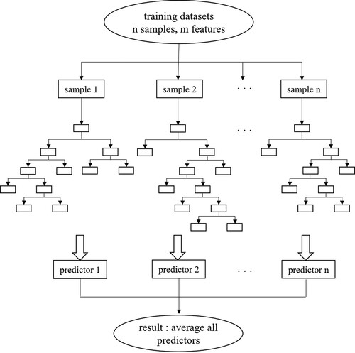
The RF algorithm, presented by Breiman (1996), is a powerful ensemble method consisting of multiple decision trees for classification and regression problems (Feng et al. 2020). Each tree continues to be split according to the minimized Gini index until it reaches the user’s preset values (Hou et al. 2020). The most essential hyperparameters include N-estimators, Max-depth, Min-samples-split, and Min-samples-leaf. The N-estimators parameter is the tree numbers of the forest, and overfitting or underfitting may occur when the n-estimators are larger or smaller than the optimal number (Ibrahim and Khatib 2017; Hou et al. 2020). The Max-depth controls the max depth of each decision tree. In addition, the Min-samples-split and Min-samples-leaf needed to be tuned, although it was found that these two hyperparameters had less impact on the performance of the RF model when N-estimators and Max-depth were determined. RF is good at dealing with nonlinear fitting and can effectively avoid overfitting (Amit and Geman 1997; Dietterich 2000). During the training process, approximately one-third of the training samples that are not used in the bootstrap process are known as out-of-bag data (OOB) (Breiman 1996; Hou et al. 2020), whose residual mean square (RMS) is used to evaluate the prediction accuracy (Gislason, Benediktsson, and Sveinsson 2006). For regression problems, the RF averages all the predictors of all the regression trees. Note that the RF method was carried out using the scikit-learn toolbox in this study (Pedregosa et al. 2011), and the structure of the RF is displayed in Figure 1.

Figure 1. Structure of the random forest (RF) method.

2.1.1.2. Adaptive boosting (AdaBoost)

The AdaBoost algorithm, proposed by Freund and Schapire (1997), is a powerful nonlinear ensemble tool. Compared with the bagging algorithm, in which the training samples are obtained independently relative to the previous step, the training samples of AdaBoost are obtained sequentially in the adaptive boosting ensemble algorithm (Thongkam, Xu, and Zhang 2008; Guo et al. 2012; Hassan et al. 2017). Specifically, the AdaBoost iterative algorithm includes three steps: (1) Initialize the weight distribution of the training samples. For example, if there are N samples, each training sample is initially assigned the same weight as 1/N. (2) Train the weak learner. For example, in a specific classification task during the training process, if a training sample has been accurately classified, its weight will be reduced in the construction of the next training set. Conversely, its weight will increase. Then, the sample set with updated weights is used to train the next classifier, and the whole training process continues iteratively. (3) Last, all the trainer weak classifiers are combined into strong classifiers. The weights of the weak classifiers with small classification error rates are increased to make them play a more decisive role in the final classification function; otherwise, they decrease. In other words, the weak classifiers with low error rates have relatively large weights in the final classifier; otherwise, they are small. In addition to the four hyperparameters, N-estimators, Max-depth, Min-samples-split and Min-samples-leaf, which have the same meaning as RF, two more essential hyperparameters, the Learning rate and Loss function, need to be determined in AdaBoost. The Learning rate represents the convergence rate of the gradient direction, and the Loss function stands for the error processing methods of the samples in the weak classifiers, which include the ‘linear’, ‘square’ and ‘exponential’. In the study, the AdaBoost module was carried out using the scikit-learn toolbox (Pedregosa et al. 2011).

2.1.1.3. Extreme gradient boosting (XGBoost)

The XGBoost algorithm is a relatively new machine learning ensemble algorithm proposed by Chen and Guestrin (2016), which is a novel implementation model based on the GBDT and RF models. Specifically, compared with an ordinary GBDT, it explicitly adds the complexity of the tree model to the optimization objective as a regular term. In addition, it draws on the idea of RF and uses feature sampling to prevent overfitting. During the training process, parallel calculations are automatically executed for the functions in the XGBoost model (Fan et al. 2019). The general function for the prediction at step t is presented as: (3) $f_i^{\left(t\right)}=\sum _{k=1}^t{f}_k\left(x_i\right)=f_i^{\left(t-1\right)}+f_i\left(x_i\right)$(3) where $f_t\left(x_i\right)$ is the learner at step t, $f_i^{\left(t\right)}$ and $f_i^{\left(t-1\right)}$ are the predictions at steps t and t-1, and $x_i$ is the input variable. The most influential hyperparameters in XGBoost modeling of a single weak learner are ‘Booster’, ‘Subsample’ and ‘Learning rate’, except for the four hyperparameters mentioned above that are common to a single decision tree, such as N-estimators, Max-depth, Min-samples-split and Min-samples-leaf. Specifically, ‘Booster’ has two options, namely, ‘gbtree’ and ‘gblinear’, which represent tree-based and linear models, respectively. ‘Subsample’ represents the proportion of samples used for training and can help prevent overfitting, and the Learning rate has the same meaning as in AdaBoost. In this study, the xgboost package in the Python platform was used to conduct the XGBoost-based net radiation estimation.

2.1.2. Artificial neural networks (ANN)

An artificial neural network (ANN) is a type of computing system inspired by the biological neural network. It consists of a layered arrangement of individual computation units called artificial neurons (Ferreira et al. 2011; Wu and Ying 2019). A standard ANN model usually consists of an input layer, one or more hidden layers, and an output layer. The inputs are fed through the hidden layer and are connected to the output layer through a series of weight combinations (Brown et al. 2020). The outputs of the output layer make a comparison to the desired outputs and update the weights through an error back propagation (LeCun, Bengio, and Hinton 2015).

2.1.2.1. Multilayer perceptron neural network (MLP)

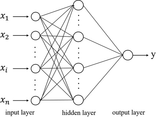
MLP is perhaps the most widespread type of feedforward network for solving classification and regression problems in many fields (Bishop 1995; Behrang et al. 2010). Back-propagation (BP) is the core algorithm of multilayer feedforward neural networks (Wang and Xu 2005). Figure 2 shows a typical neural network consisting of three layers, an input layer, a hidden layer and an output layer. Many studies have shown that one hidden layer is sufficient to solve most problems (Mas and Flores 2008; Xu et al. 2021), so this study applies a typical three-layer neural network to estimate $R_n$. In addition, hyperparameters such as the number of neurons in the hidden layer, activation function and batch size have significant effects on the performance of an MLP. Specifically, an overly low number of neurons in the hidden layer usually makes the network perform underfitting, while an overly high number may result in overfitting (Yeom et al. 2019). Activation functions are used to enhance the nonlinear expression ability of neural networks, and the commonly used nonlinear activation functions include the hyperbolic tangent function (Tanh) (Zhang, Gao, and Song 2016a), sigmoid function (Tsai et al. 2015) and rectified linear units (ReLU) (Wang, Zeng, and Lin 2021). However, when the collected dataset is large, the MLP needs to be trained in batches, and the Batch size refers to the number of samples for one training process, which affects the optimization effect and training speed of the trained model. In this study, the deep learning application programmer interface (API) of ‘Keras’ in the Python platform was used to conduct an MLP-based net radiation estimation.

Figure 2. Structure of the multilayer perceptron neural network (MLP) method.

2.1.2.2. Radial basis function neural network (RBF)

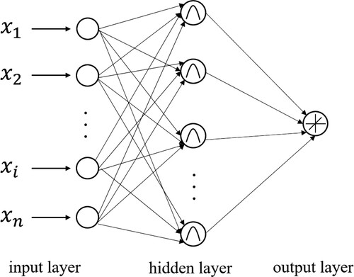
The RBF network is a popular type of network that is widely applied to pattern classification problems (Bishop 1995), and the structure of the RBF is displayed in Figure 3. The radial basis function is a real value function whose value depends only on the distance from the origin, and any activation function that satisfies this characteristic is called the radial basis function, the most commonly used is the Gaussian kernel function, which is also called the RBF kernel. The main difference between the RBF and MLP networks is the activation function of the hidden layer. Specifically, the RBF makes the output of its network related to the partial modulation parameters, which means that the farther the input of the neuron is from the center of the radial basis function, the lower the degree of activation of the neuron. When training the RBF model, two essential hyperparameters need to be determined, namely of the Neurons of the hidden layer and Gamma. The former represents the number of centers of the hidden layer basis function, which is usually determined by the K-means method (Yuchechen et al. 2020), while the latter is used to control the scope of influence of the RBF kernel. In general, with an increase in the number of neurons in the hidden layer, the performance of the RBF improves but the training time also increases dramatically, and there may be an overfitting phenomenon. During prediction, the output of the RBF network is based on a linear combination between the inputs of the RBF and neuron parameters (Kisi et al. 2020).

Figure 3. Structure of the radial basis function neural network (RBF) method.

2.1.3. Kernel methods - support vector machine (SVM)

SVM is a statistical learning theory based on structural risk minimization developed by Vapnik (Sain 1996), which is widely used due to its powerful nonlinear regression capability (Mountrakis, Im, and Ogole 2011; Fan et al. 2019). Support vector regression (SVR), the regression version of SVM, is well suited for modeling small samples owing to its powerful predictability (Mountrakis, Im, and Ogole 2011). The SVR model predicts the regression values through various kernel functions that implicitly convert the original low-dimensional input data into a high-dimensional feature space for linear segmentation (Fan et al. 2018). Compared with an artificial neural network, which easily converges to a local optimum (Chen, Li, and Wu 2013), the SVM gives a unique solution resulting from the convex nature of the optimality problem (Fan et al. 2018). Moreover, by introducing regularization parameters, SVM can effectively overcome the overfitting problem. Therefore, the SVM can better solve the problems of small samples, nonlinearity and high dimensionality and is often used for identification and prediction. However, it should be noted that SVM is more suitable for small samples due to its high computational complexity (Feng et al. 2020), so there is research value in exploring the performance of SVM in large samples. The kernel function is an essential hyperparameter that affects the performance of SVM, which is used to compute the inner product after converting to higher dimensional space, and if the RBF kernel is used, the Gamma must be determined, which has the same meaning as does in the RBF model. In this study, the ‘SVR’ package in the Python platform on the scikit-learn platform was used to conduct SVM-based net radiation estimations (Pedregosa et al. 2011).

2.2. Three DL methods

Deep learning (DL) methods generally represent neural networks with large-sizes and deep layers (Yuan et al. 2020) compared with the traditional machine learning methods above; they help capture the potential relationship between multiple variables and dependent variables owing to multilayer learning (Bengio, Courville, and Vincent 2013; LeCun, Bengio, and Hinton 2015).

2.2.1. Multilayer perceptron neural network with stacked autoencoders (SAE)

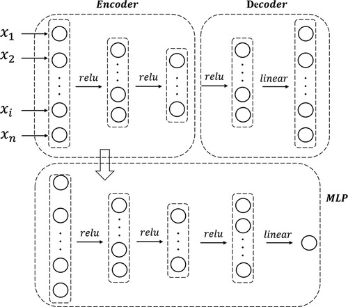
An autoencoder is a type of neural network with a symmetrical structure from encoding to decoding layers with the same numbers of input and output dimensions in an unsupervised or supervised manner (Wang and Liu 2018; Zhang et al. 2020). The encoder layers, as shown in Figure 4, can adaptively learn the abstract features of input data and then represent the complex data in an efficient manner by minimizing the errors between the outputs of the decoder layer and the inputs of the encoder layer. These properties make the autoencoder not only suitable for large samples of data but also effectively reduce the design costs and improve the traditional poor generalizations. Therefore, using the autoencoder algorithm in a deep neural network can efficiently extract the implicit features and yield better estimation results based on an MLP connected behind the autoencoder module. Specifically, the accuracy performance of the SAE model is significantly affected by the construction of the encoder/decoder, neurons of the hidden layer, activation function and Batch size, which will be determined in Section 4.1.

Figure 4. Structure of the stacked autoencoders (SAE) method.

2.2.2. Deep belief network (DBN)

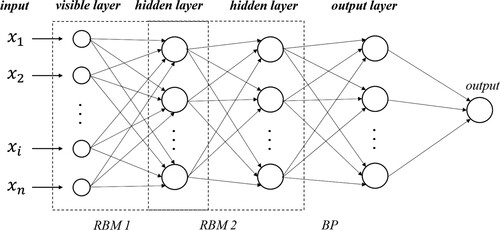
The DBN is one of the most popular deep learning models (Hinton, Osindero, and Teh 2006; Li et al. 2017; Zang et al. 2020) and was proposed by Hinton, Osindero, and Teh (2006). As a Bayesian probabilistic generation model, DBN is generally composed of multiple restricted Boltzmann machine (RBM) layers and a BP layer. Figure 5 shows the structure of the DBN with two RBM layers and one BP layer as an example. The RBM is an energy-based model that can avoid local optima problems and vanishing gradients by pretraining the weights of the dense layers (Hinton, Osindero, and Teh 2006). Specifically, the significance of training an RBM is adjusting the parameters of the model to fit the given input data by a contrastive divergence (CD) and ultimately making the probability distribution of the visible units consistent with the input data (Shen et al. 2020; Wang et al. 2020). An RBM contains a visible layer and a hidden layer, where the hidden layer of the prior RBM is the visible layer of the next RBM (Shen et al. 2018), and the BP layer is usually utilized for a classification or regression, and has the same functions as the MLP module in SAE. Specifically, in addition to the Batch size and Activation function, three important hyperparameters need to be determined for the DBN, namely, the construction of the RBM layers and hidden layers and the learning rate of the RBM layer in the training process.

Figure 5. Structure of the deep belief network (DBN) method.

2.2.3. Residual neural network (ResNet)

Inspired by the very powerful nonlinear representation ability of CNNs, DL algorithms have seen a dramatic rise in popularity for remote-sensing image analysis over the past few years (Zhang, Zhang, and Du 2016b; Kussul et al. 2017; Wu et al. 2019; Yuan et al. 2020). CNNs are biologically inspired variants of multilayer perceptrons that can hierarchically extract powerful low-level and high-level features (LeCun, Bengio, and Hinton 2015; Jiang et al. 2019). A standard CNN is mainly composed of an input layer, a convolutional layer, a pooling layer, a fully connected layer, and an output layer. It should be noted that several convolutional layers and pooled layers can be alternately arranged to form multiple CNNs (Tan et al. 2019). The convolution layer is used to extract local features using local connections and a sharing of the weights (LeCun, Bengio, and Hinton 2015; Aghdam and Heravi 2017), and the pooling layer is used to reduce the number of training parameters in the deep neural network. The feature map is produced by sharing the kernel weights and biases within the receptive field through a sliding convolutional kernel across the entire input imagery. The fully connected layer is used to integrate the local features extracted by the previous convolution layer (Wang et al. 2020). Two convolutional layers are usually connected by a nonlinear layer, which is actually an elementwise operation applying a nonlinear activation function to each value in the feature maps (Jiang et al. 2019). The ReLU (Nair and Hinton 2010; Krizhevsky, Sutskever, and Hinton 2012; Romanuke 2017), which makes the nonpositive values zero and keeps the positive values unchanged, is used in the proposed ResNet model, as it is effective in alleviating the notorious vanishing gradient problem and speeding up the learning process. In addition, a batch normalization layer is usually needed between the convolutional layers and the nonlinear layer to speed up the training of the convolutional neural network and reduce the sensitivity to network initialization (Ioffe and Szegedy 2015).

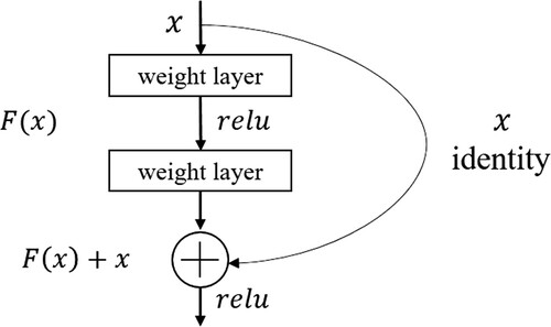
However, deep neural networks are often difficult to train well because CNNs usually face the obstacles of performance degradation problems and vanishing or exploding gradients. Thus, the residual learning technique proposed by He in 2016 (He et al. 2016) has been introduced in deep CNNs to solve these problems. The original directly fitted a desired underlying mapping $\mathrm{H}\left(\mathrm{x}\right)$ for each few stacked layers; nevertheless, the stacked nonlinear layers in the residual modules fit a residual mapping $\mathrm{F}\left(\mathrm{x}\right)=\mathrm{H}\left(\mathrm{x}\right)-x$ and output function $\mathrm{F}\left(\mathrm{x}\right)+x$ with a shortcut connection from the inputs, as shown in Figure 6. With the help of a residual learning algorithm, deep CNNs are easier to optimize and give better results (Lim et al. 2017). In this study, the Python deep learning API of ‘Keras’ was used to conduct ResNet-based net radiation estimations.

Figure 6. Structure of residual block.

3. Data and methodology

3.1. Data and pre-processing

Three types of datasets are used in this study as in our previous study (Li et al. 2021), including the TOA band observations from MODIS, daily $R_n$ from ERA5 reanalysis data, and ground daily $R_n$ measurements collected from more than 300 globally distributed sites at mid-low latitudes. In addition, the GLASS-MODIS $R_n$ product was used for intercomparison. For a more comprehensive evaluation, the daily $R_n$ measurements from seven sites located in the rugged terrain area in China were collected and used for further validation.

3.1.1. Ground measurements

3.1.1.1. From 340 sites at the flat surface

Comprehensive daily $R_n$ measurements from 2000 to 2017 from 340 sites distributed at mid-low latitudes (${60}^{{}^{\circ }}$S –${60}^{{}^{\circ }}$N) in thirteen measuring networks were collected for modeling and validation (see Table 1), and these sites were all at relatively flat surfaces (Li et al. 2021). Figure 7 presents the spatial distribution of these sites located in various climate zones defined by the Köppen–Geiger climate classification (Peel, Finlayson, and McMahon 2007) and the quantitative distribution of the various land cover types and climate zones to which they belong. Statistically, the 340 sites were under fourteen land cover types defined by the International Geosphere-Biosphere Program (IGBP) (Loveland and Belward 1997), including croplands < CRO>, grasslands < GRA>, deciduous broadleaf < DBF>, urban and built up < URB>, mixed forests < MF>, open shrublands < OSH>, evergreen broadleaf < EBF>, deciduous needleleaf < DNF>, permanent wetlands < WET>, evergreen needleleaf < ENF>, barren sparse vegetation < BSV>, woody savannas < WSA>, savannas < SAV>, and closed shrublands < CSH>, and their elevations ranged from −7 m to 4698 m above sea level. Therefore, the ground measurements collected in this study were comprehensive because they are located across the global mid-low latitudes and represent a variety of climate types, land cover types and elevation ranges.

Figure 7. (a) Geographical distribution of the 340 sites in 13 measurement networks and the climate zones these sites belong to, (b) the proportion of fourteen site land cover types, and (c) the proportion of the five climate types of the 340 sites.

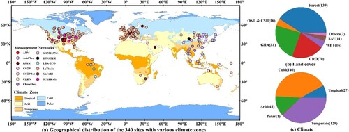
Table 1. Information about the thirteen measuring networks.

Abbreviation	No. of sites	Time Span	Instrument	Temporal resolution	Reference
ARM^1	33	2001–2017	Kipp&Zonen Pyrgeometer	1 min	(Phillips et al. 2017)
AsiaFlux	26	2001–2015	Kipp&Zonen, CM-6F	30 min	(Shi and Liang 2013)
BSRN^2	7	2001–2017	Eppley, PIR/Kipp&Zonen CG4	1 or 3min	(Zo et al. 2017)
CEOP^3	8	2008–2009	Eppley PIR, CG4	30 min	(Yao et al. 2014)
CEOP_Int	5	2002–2019	QMN101	30 min	\
CERN^4	1	2007–2014	–	30min	(Fu et al. 2010)
ChinaFlux	3	2003–2016	–	30min	\
GAME.ANN	2	2001–2003	EKO MS0202F	30 min	\
HiWATER	16	2012–2012	CNR-4	10 min	(Shaomin et al. 2012)
LaThuile^5	227	2001–2017	Kipp&ZonenCNR-1,etc	30 min	(Ornl 2015)
LBA-ECO^6	4	2001–2006	REBS Q*7.1	1 h	(Tóta et al. 2008)
SAFARI^7	1	2001–2017	Kipp&Zonen Pyrgeometer	30 min	(Swap et al. 2003)
SURFRAD	7	2001–2017	Eppley, PIR	3 min	(Augustine, DeLuisi, and Long 2000)

¹ ARM: Atmospheric Radiation Measurement (Phillips et al. 2017), ²BSRN: Baseline Surface Radiation Network (Zo et al. 2017), ³CEOP: Coordinated Enhanced Observation Network of China (Yao et al. 2014), ⁴CERN: Chinese ecosystem research network (Fu et al. 2010), ⁵LaThuile: Global Fluxnet (LaThuile dataset) (Ornl 2015), ⁶LBA-ECO (Large Scale Biosphere-Atmosphere Experiment) (Tóta et al. 2008), ⁷SAFARI: Southern African Regional Science Initiative Project (Swap et al. 2003).

To ensure the quality of the site measurements, only the measurements labeled as high quality by their releasers were used. Since the observation frequency of each measurement network is different, the daily $R_n$ values were calculated only when there was at least one valid observation within half an hour in one day (Jiang et al. 2014; Li et al. 2021). After matching with the corresponding MODIS TOA observations, a total of 664,974 daily $R_n$ samples were collected, which were further divided into training and independent validation datasets. To ensure a reasonable and similar distribution of these two datasets, 80% of the measurements at each site were randomly selected for training (488,390 samples in total), and the remaining 20% were selected for validation (176,584 samples in total).

3.1.1.2. From 7 sites in the rugged terrain area

According to previous studies (Yan et al. 2018; Yan et al. 2020), the influence of the topography on radiative component estimations is significant because of shadows and multiscattering. Therefore, the ground measurements from seven sites located at the Moon Mountain of the Saihanba Forest Park (42${}^{\circ }$23’N, 117${}^{\circ }$24’E) in Chengde city, northeast China (Yan et al. 2018; Yan et al. 2020), were collected from August 2018 to May 2020 to explore how these machine learning models work in a rugged terrain area. Table 2 provides detailed information of the seven sites, and Figure 8 shows their topography distribution, which was acquired from the DEM data provided by the National Aeronautics and Space Administration (NASA) Shuttle Radar Topographic Mission (SRTM). The elevation of the 7 sites ranges from ∼1700m to ∼ 1800m with GRA land cover but these sites were located at various slopes and aspects. The CNR4 net radiometers applied for measuring at the 7 sites were set parallel to the inclined western or southern surfaces for measuring more reasonably at rugged terrain areas. More detailed information can be found in Yan et al. (2018). The original measurements were at a frequency of 1 min, and they were processed into daily averages like those from the 340 sites. After matching with the MODIS TOA observations, 2,982 samples were obtained for validation.

Figure 8. (a) Geographical location and (b) the corresponding DEM distribution of the 7 sites (dark spots) at Chengde mountainous area.

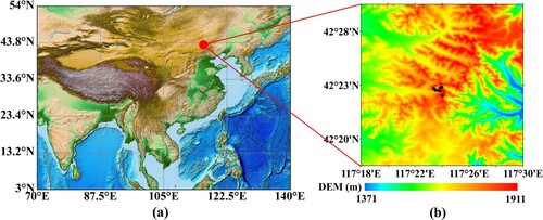
Table 2. The detailed information about the seven mountainous stations in Chengde city in China.

Station	Latitude(${}^{\circ }$)	Longitude(${}^{\circ }$)	Elevation(m)	Slope(${}^{\circ }$)	Aspect(${}^{\circ }$)	IGBP
1	42.397	117.399	1848.551	9	85	GRA
2	42.397	117.398	1848.427	19	269	GRA
3	42.393	117.397	1852.700	26	196	GRA
4	42.393	117.395	1810.066	22	285	GRA
5	42.394	117.392	1700.166	2	47	GRA
6	42.396	117.390	1756.811	29	189	GRA
7	42.387	117.400	1838.169	30	138	GRA

3.1.2. Remotely sensed datasets

3.1.2.1. MODIS products

The MODIS sensors are aboard the Terra and Aqua satellites operated by NASA, providing the MOD and MYD series products, with a 10:30 equatorial crossing time and 13:30 equatorial crossing time during the daytime, respectively (Wu and Ying 2019). Both the Terra and Aqua satellites provide the opportunity to observe the entire Earth’s surface every one or two days for 36 spectral bands in wavelengths from 0.405–14.385 µm. As in the study of Li et al. (2021), the MOD and MYD series products, including the TOA reflectance and irradiance from MOD/MYD021KM and the corresponding geometric information from MOD/MYD03, were used in this study, and the detailed information is given in Table 3. All MODIS products were extracted according to the site locations and quality control as specified by Li et al. (2021).

Table 3. The MODIS products used in this study.

MODIS Product	Temporal Resolution	Spatial Resolution	Variables Used
MOD/MYD02	5 min	1 km	1 km_RefSB,1 km_Emissive
MOD/MYD03	5 min	1 km	SolarZenith(SZA),SolarAzimuth(SAA), SensorZenith(VZA),SensorAzimuth (VAA), Height

3.1.2.2. GLASS-MODIS daily Rn product

Similar to the GLASS-MODIS daytime $R_n$ product (Jiang et al. 2016), the GLASS-MODIS daily $R_n$ product at 0.05° since 2000 was also mainly generated based on the close relationship between $R_s^{\downarrow }$ and $R_n$ with other ancillary information over the global regions where $R_s^{\downarrow }$ was available covering almost all areas at mid-low latitudes. After validating against comprehensive in situ measurements all over the globe, the performance of GLASS-MODIS daily $R_n$ was superior to the other products, with an overall validation root-mean-square error (RMSE) of 26.18 Wm⁻² (Jiang et al. 2016). Guo et al. (2020) applied the GLASS-MODIS daily $R_n$ for ET estimation and achieved a better accuracy than using the daily $R_n$ from the MERRA2 reanalysis product. In this study, GLASS-MODIS daily $R_n$ were extracted according to site locations and measuring times of the validation samples for model evaluations.

3.1.3. Daily ${\mathit{R}}_{\mathit{n}}$ from the ERA5 reanalysis product

As the newest generation of reanalysis products updated from ERA-interim (Dee et al. 2011; Hersbach et al. 2020), ERA5 provides high-quality global land surface, oceanic and atmospheric reanalysis datasets at an hourly resolution with a spatial resolution of 25 km (Hersbach et al. 2020). Its radiative components are generated based on radiative transfer models (RTMs), and the validation results indicated that the radiative components from ERA5 performed better than ERA-Interim and MERRA2 (Martens et al. 2020; Sianturi and Marjuki Kwarti 2020). The ERA5 daily average $R_n$ was calculated by aggregating the hourly $R_n$ values calculated by adding the four hourly radiative components. Similar to Li et al. (2021), the ERA5 daily $R_n$ extracted according to samples was also introduced as a physical constraint into the $R_n$ estimation model based on MODIS TOA observations to improve the estimation accuracy at mid-low latitudes.

3.2. Methodology

According to Li et al. (2021), the accuracy of the estimated daily $R_n$ at mid-low latitudes directly from the MODIS TOA observations would be improved significantly by incorporating the ERA5 daily $R_n$, which could provide additional information that the limited available MODIS TOA data cannot provide in this region. The daily $R_n$ at mid-low latitudes is estimated as follows: (2) $R_n=f\left(TO{A}_{ref},TO{A}_{rad},SZA,VZA,RAA,height,d_r,\phi ,R_{n\mathrm{\_}ERA5}\right)$(2) (2a) $d_r=1+0.033\ast \mathrm{c}\mathrm{o}\mathrm{s}\left({\displaystyle \frac{2\pi doy}{365}}\right)$(2a) where $TO{A}_{ref}$ and $TO{A}_{rad}$ are the MODIS TOA reflectance data (bands 1-5, 7, 19) and radiance data (bands 21, 24, 25, 27-36) from MOD/MYD02 1 km during daytime. $SZA$, $VZA$, $RAA$ and $height$ are the solar zenith angle (°), sensor azimuth (°), relative azimuth (the absolute value of solar azimuth minus sensor azimuth) (°) and height (meter) obtained from MOD/MYD03. $R_{n\mathrm{\_}ERA5}$ is the daily $R_n$ from ERA5 and $d_r$ is the inverse relative distance from the Earth to the Sun calculated by Eq. (2a). $\phi$ is the latitude (°) of the sites and $doy$ is the day of the year. The final daily $R_n$ was the average of all the estimated values in one day, the number of which was determined by the overpass times of MODIS during the daytime. In this study, the nine evaluated ML methods were employed by this equation one by one, and all the models were implemented with a Microsoft Windows 10 system on a Inter Core 3.20 GHz PC with 32 GB memory. Section 4.1 presents the tuning process of each of the nine models.

Afterwards, the performance of the nine models was evaluated by validating against the ground measurements and making comparisons with the GLASS-MODIS daily $R_n$. Four commonly used statistical indices were employed to represent accuracy, the determination coefficient ($R^2$), root mean square error (RMSE), bias, and relative root mean square error (rRSME), and are given as follows: (3a) $R^2=1-{\displaystyle \frac{{\sum }_{i=1}^n{\left(e_i-o_i\right)}^2}{{\sum }_{i=1}^n{\left(o_i-\overline{o}\right)}^2}}$(3a) (3b) $RMSE=\sqrt{{\displaystyle \frac{1}{n}\sum _{i=1}^n{\left(o_i-e_i\right)}^2}}$(3b) (3c) $Bias={\displaystyle \frac{1}{n}\sum _{i=1}^n\left(e_i-o_i\right)}$(3c) (3d) $rRMSE={\displaystyle \frac{RMSE}{mean\left(X\right)}}$(3d) where $e_i$ is the estimated daily $R_n$, $o_i$ is the ground measurement, and X represents all the site observations. The rRMSE was used to eliminate the influence on the validation accuracy caused by the unbalanced sample sizes of various types.

Finally, the influencing factors (i.e. land cover, elevation, topography and sample size), the mapping ability, and the efficiency and requirements for the operating environment or hardware of the nine models were further analysed and discussed.

4. Results and analysis

4.1. Tuning of the nine ML models

To obtain the best models, the hyperparameters of each model described in Section 2 were tuned. The detailed information is as follows.

4.1.1. ML methods

4.1.1.1. Tree methods

Three tree methods (RF, AdaBoost, and XGBoost) were applied in the present study. As mentioned in Section 2, four hyperparameters, including ‘N-estimators’, ‘Max-depth’, ‘Min-samples-split’ and ‘Min-samples-leaf’, all need to be tuned for RF, AdaBoost, and XGBoost modeling. In addition, two more hyperparameters, ‘Learning rate’ and ‘Loss’, are needed for AdaBoost, whereas three hyperparameters, ‘Booster’, ‘Subsample’ and ‘Learning rate’, are needed for XGBoost. After multiple experiments, the threshold settings for all the hyperparameters of the three tree methods are shown in Table 4. The threshold values of all the hyperparameters were set as [minimum value, by step, maximum value] except the ‘Learning rate’, ‘Loss’ and ‘Booster’. For instance, the values for the ‘N-estimators’ were defined as [30, 10, 100], which means that the value of the ‘N-estimator’ for the three tree methods ranged from 30∼100, and the values 30, 40, 50, 60, 70, 80, 90 and 100 by steps of 10 were traversed to determine this hyperparameter. Based on the same training and validation samples, the best combination of hyperparameters for the three tree models were determined and given in parentheses or highlighted in red in Table 4. Note that some hyperparameters have little effect on the three models, such as ‘Min-samples-split’ and ‘Min-samples-leaf’.

Table 4. Hyperparameters setting for determining the optimal RF, AdaBoost and XGBoost models. The value in parentheses or highlighted by red was the determined value for each of the hyperparameters for the optimal three models.

Hyperparameters		Tree Model
	RF	AdaBoost	XGBoost
N-estimators	[30, 10, 100] (50)	[30, 10, 100] (50)	[30, 10, 100] (60)
Max-depth	[5, 1, 14] (11)	[5, 1, 14] (9)	[5, 1, 14] (6)
Min-samples-split	[3, 1, 8] (6)	[3, 1, 8] (6)	[3, 1, 8] (5)
Min-samples-leaf	[3, 1, 8] (5)	[3, 1, 8] (4)	[3, 1, 8] (4)
Learning rate	\	{0.001,0.01,0.1}(0.1)	[0.05, 0.05, 0.55] (0.3)
Loss function	\	linear/square/exponential	\
Subsample	\	\	[0.6, 0.1, 1] (1)
Booster	\	\	gbtree/gblinear

4.1.1.2. ANN

A three-layer network architecture was applied for the MLP and RBF models (Broomhead and Lowe 1988), which means that the two models both contained one input layer, one hidden layer and one output layer. In addition to the number of neurons in the hidden layer being the common hyperparameter to be set in the two models, the other hyperparameters need to be determined separately for the two methods, such as the hyperparmeters ‘Activation function’ and the ‘Batch size’ for MLP and ‘Gamma’ for RBF (see Table 5). Moreover, the widely used Adam optimizer is applied in MLP modeling for iterative training to optimize the weights and biases in the hidden layer to reduce the optimization cost (Kingma and Ba 2014), and the RBF kernel is used in the RBF model.

Table 5. The same as Table 4 but for the MLP and RBF models.

Hyperparameters	Values
	MLP	RBF
Neurons of the hidden layer	[5, 5, 100] (65)	[100, 100, 800] (800)
Activation function	Relu/Tanh/Sigmoid	\
Kernel	\	RBF
Batch size	{32,64,128,256,512,1024} (512)	\
Gamma	\	{0.0001,0.001,0.01,0.1} (0.001)

4.1.1.3. SVM

The common kernel functions used in the SVM model include linear, polynomial, RBF and sigmoid, and the RBF kernel was applied because it performs better than other kernel functions in regression cases after multiple experiments. Similar to the RBF model, Gamma is the most important hyperparameter to be set. The detailed hyperparameters settings are shown in Table 6.

Table 6. The same as Table 4 but for the SVM model.

Hyperparameters	values
Kernel	linear/polynomial/RBF/sigmoid
Gamma (only for RBF)	{0.00001,0.0001,0.001,0.01,0.1} (0.0001)

4.1.2. DL methods

4.1.2.1. SAE

There are four hyperparameters to be determined in SAE, and the most essential are the number of neurons and network layers structure in the encoder/decoder layer and the hidden layer in MLP, and the other two are the ‘Activation function’ and ‘Batch size’. To reduce the tuning cost, a single layer was used for both the encoding/decoder layer and the hidden layer in the MLP. Table 7 lists the settings of these hyperparameters and the determined hyperparameters.

Table 7. The same as Table 4 but for the SAE model.

Hyperparameters	values
Neurons of the encoder layer	[5, 5, 90] (60)
Neurons of the hidden layer	[5, 5, 90] (80)
Activation function	Relu/Tanh/Sigmoid
Batch size	{64,128,256,512,1024,2048} (256)

4.1.2.2. DBN

A previous study indicated that a one-layer RBM was enough to achieve satisfactory accuracy (Wang et al. 2020). Hence, one RBM and one hidden layer were applied in the DBN modeling. Table 8 gives detailed information about the hyperparameter settings in the DBN. Note that the iterative training times for the RBM and hidden layer also affect the final accuracy of the DBN, with the accuracy and training cost increasing when the training times increase. To trade off the training cost and accuracy performance, the iterative times for the RBM layer and hidden layer were finally set as 100 and 1200 times in the present study.

Table 8. The same as Table 4 but for the DBN model.

Hyperparameters	values
Neurons of the hidden layer	{16,32,64,128,256} (256)
Learning rate of RBM	{0.001,0.01,0.1} (0.1)
Activation function	Relu/Tanh/Sigmoid
Batch size	{64,128,256,512,1024,2048} (256)

4.1.2.3. ResNet

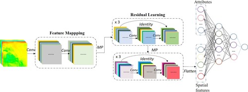
Figure 9 shows a schematic diagram of the proposed ResNet model, which uses the study of Jiang et al. (2019) as a reference. It shows that the input to ResNet is an image block with a format of height × width × channels, in which the channels were set to 20 according to the numbers of bands in Eq. (2)(1a) $R_{ns}=R_s^{\downarrow }-R_s^{\uparrow }=\left(1-\alpha \right)R_s^{\downarrow }$(1a) , and then, the two sequential convolution layers were set to 32 kernels with a 3 × 3 size, and a max-pooling layer was set to a stride of 2 with a 2 × 2 kernel size, which were applied to downsample the input image block. After that, the downsampling feature maps entered into the residual learning blocks equipped with 64 and 128 kernels with a 3 × 3 size, respectively, and the learning process for each residual module was repeated three times. Last, the flattened spatial pattern combined with the auxiliary information at the center pixel entered into the MLP module equipped with two hidden layers with 128 and 64 neurons.

Figure 9. Structure of the residual neural network (Jiang et al. 2019).

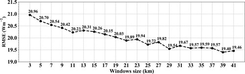
According to previous studies, the window size of the input image block could reflect the influence of the spatial scale on an $R_n$ at a central pixel (Jiang et al. 2020), and the spatial scale is related to the heterogeneity of the underlying surface and the temporal resolution of the samples (Li et al. 2005; Wang et al. 2015a; Huang et al. 2016), which means that the optimal input window size would become larger if the underlying surface become more homogeneous and the sampling frequency became longer. Hence, in ResNet modeling, the most appropriate window size for the input image block should be determined first to achieve the best performance. As suggested by Wang et al. (2015b), the largest window size of the input image block should be less than 50×50 km², and the size of 41$\times$41 km² was set as the threshold in this study by considering the sites used. Then, the optimal window size could be determined by the highest validation accuracy when the size increased from 3×3–41×41 km² at an interval of 2 by using the same training samples. Figure 10 shows the variations in the validated RMSE values with the different input window sizes. The results indicated that the RMSE value gradually decreased with the increasing input window size of the MODIS images and stabilized when the window size was larger than 33×33 km². Finally, the window size was determined to be 39×39 km² in our ResNet model as the RMSE value reached the minimum (19.40 Wm⁻²).

Figure 10. The variations in the validated accuracy (represented by RMSE) in the daily ${\mathit{R}}_{\mathit{n}}$ estimations from the ResNet model when the inputted window size of MODIS images ranging from 3×3 km² to 41×41 km² with the stride of 2.

In summary, it is crucial to determine the most appropriate combination of hyperparameters to obtain an optimal ML model. Among the nine methods, the hyperparameters that need to be set in the SVM method are the fewest. Moreover, when determining the best model the issue of overfitting in ML modeling is also to be considered in addition to the minimum validation accuracy. To do this, the ML models were trained repeatedly with different combinations of hyperparameters until the difference in RMSE values from the training and validation was small ($\le$ 1 Wm⁻² in this study). Overall, tuning an ML method is a subjective process, and the obtained model is highly dependent on the samples, the experience of operators and the modeling platform.

4.2. Nine model performance intercomparisons

4.2.1. Overall validation accuracy at the site scale

The daily $R_n$ estimates from the nine determined ML models were directly validated against the independent ground measurements (No. of samples  = 176,584 samples), and the results are given in Table 9.

Table 9. Validation accuracy of the nine ML models against the independent validation ground measurements.

	Models	RMSE (Wm^−2)	bias (Wm^−2)	R^2
Classical ML methods	RF	22.81	0.09	0.88
	AdaBoost	23.08	0.08	0.88
	XGBoost	20.25	0.06	0.91
	MLP	21.37	0.97	0.90
	RBF	22.34	−0.12	0.89
	SVM	22.73	−0.40	0.88
DL methods	SAE	20.16	0.77	0.91
	DBN	21.72	0.57	0.89
	ResNet	19.40	0.14	0.92

Generally, the three DL models (SAE, DBN and ResNet) performed better than most of the classic ML models with the best and second performing ResNet and SAE models, which yielded RMSEs of 19.40 and 20.16 Wm⁻², biases of 0.14 and 0.77 Wm⁻², and R² values of 0.92 and 0.91, respectively, and the DBN model performed the worst among the three DL models but still yielded a relatively small RMSE of 21.72 Wm⁻² and a high R² of 0.89. Among the six classical ML models, the XGBoost model performed the best and was similar to the SAE model, with an RMSE of 20.25 Wm⁻², a bias of 0.06 Wm⁻², and an R² of 0.91; the MLP model yielded an RMSE of 21.37 Wm⁻², a bias of 0.97 Wm⁻² and an R² of 0.90. The other four ML models (RF, AdaBoost, RBF, and SVM) performed similarly, with RMSE values ranging from 22∼23 Wm⁻², and the performance of the RF model was coincident with the study of Li et al. (2021). Moreover, the three tree models (RF, AdaBoost and XGBoost) yielded minimal bias values between 0.06∼0.09 Wm⁻² among the nine models, which might be because of their ensemble learning characteristics. Overall, the performance of the nine ML methods in $R_n$ estimation was satisfactory.

4.2.2. Model performance under various conditions

For a more comprehensive assessment, the validation accuracy in the daily $R_n$ estimation from the nine ML models under various conditions regarding the land cover types, elevation zones, seasons and latitude zones were further examined.

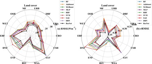
As described in Section 3.1.1, the independent validation samples were from fourteen land cover types; hence, the validation accuracy represented by RMSE and rRMSE for each land cover were compared and are shown in Figure 11. As Figure 11a shows, the ResNet model (black line with dots) performed the best for daily $R_n$ estimations for all land cover types, with RMSE values ranging from 11∼26 Wm⁻². The validation results were shown in the innermost layer, which means that the RMSE values were almost the smallest for each of the land cover types. The SAE model (red line with dots) and XGBoost model (dark green line with dots) followed with similar performances, with RMSE values ranging from 12∼28 Wm⁻² and 13∼28 Wm⁻², respectively. Other ML models, such as MLP, RBF, SVM, AdaBoost and DBN, performed worse but similarly, with RMSE values ranging from 13∼33 Wm⁻², and the results were in accordance with the results in Section 4.2.1. Combined with the results in Figure 11b, which eliminated the influence of different sample sizes, the nine ML models performed better when the land surface was covered with sparse vegetation, such as BSV and URB, followed by OSH and CSH, while almost all the models performed poorly for SAV and some forest types, including MF, DBF, ENF and DNF, and the discrepancy in model performance was the largest for DNF, with rRMSE values ranging from 0.28∼0.39 (RMSE values ranging from 20.4∼28.7 Wm⁻²). It was assumed that the poor performance for SAV, DNF and ENF for the nine ML methods might be caused by the small size of the training samples as compared to the other land cover types (such as 767 for SAV and 2,085 for DNF). In addition, it is also reported that the estimated accuracy of the other parameters (i.e. ET and $R_{ns}$) was also poor in dense forest types such as ENF and DNF (Yao et al. 2015; Wang et al. 2019), possibly due to their special growth environment.

Figure 11. The performance of the nine ML models in daily ${\mathit{R}}_{\mathit{n}}$ estimation at fourteen land cover types represented by (a) RMSE (Wm⁻²) and (b) rRMSE.

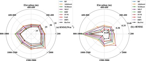
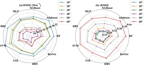
Figure 12a-b shows the validated RMSE and rRMSE of the nine ML models for eight elevation zones (<200 m, 200–400 m, 400–600 m, 600–800 m, 800–1000 m, 1000-1500 m, 1500-2000m and > 2000m), respectively. The results indicate that the performance of the nine ML models was relatively robust but was generally getting worse as the elevation increased, with their RMSE values increasing from ∼20 Wm⁻² for elevations smaller than 800 m to 20∼30 Wm⁻² for other elevation zones (Figure 12a), and the worst performance for these models was shown at the 800–1000 m and >2000m elevation zones. As before, the ResNet model still performed the best across all the elevation zones, followed by the SAE and XGBoost models, and the AdaBoost and SVM models performed the worst.

Figure 12. The same as Figure 11 but for various elevation zones.

The model performance in the four seasons and in different latitudes is shown in Figures 13 and 14, respectively. The four seasons in the Northern Hemisphere were defined as spring from March to May, summer from June to August, autumn from September to November, and winter from December to February in the following year. From the two figures, the uncertainty in the daily $R_n$ estimated by all the ML models was relatively larger in the winter season and at mid-high latitudes, with rRMSE values of 0.86∼1 for winter days and 0.25∼0.37 for latitudes higher than 40°; however, the validated RMSE values under the two conditions were not large, with values of 14.3∼17 Wm⁻² and 19.8∼23.8 Wm⁻², respectively, which was assumed to be due to the influence of snow/ice and clouds, the accuracy of the ERA5 daily $R_n$, and the number of samples used for training. Similar to other results, the ResNet model still performed the best, followed by the SAE and XGBoost models.

Figure 13. The same as Figure 11 but for the four seasons in the Northern Hemisphere.

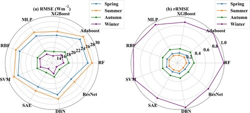
Figure 14. The same as Figure 11 but for the different latitude zones in the Northern Hemisphere, where 10°, 20°, 30°, 40°, 50° and 60° represent the validation accuracy at 10° intervals, for example, 40° represents the range from 30° to 40°.

Overall, similar to the overall validation accuracy, among the nine models, ResNet performed the most robustly and the best across almost all the land cover types, elevation ranges, seasons and latitude zones, followed by SAE and XGBoost. However, nearly all the models performed unsatisfactorily at some land cover types (e.g. SAV, ENF, DNF), some elevation zones (800–1000 m, > 2000m), winter days, and mid-high latitudes owing to the limited number of available training samples, poor accuracy of the ERA5 $R_n$ and so on (Wang et al. 2019).

4.2.3. Model implementation cost

In addition to the estimation accuracy, one of the issues that concern users the most is the resources needed for model implementations in practice, particularly the requirements on the hardware and the model’s running efficiency. In this study, it was found that the time needed for $R_n$ predictions of all the nine ML models was within seconds except for the ResNet model but it was still less than half an hour. Hence, the time needed for model training and the memory required for the running of the nine models were recorded and are presented in Figure 15.

Figure 15. The computational cost of the nine models represented by (a) the time spent for training and (b) the memory needed for model running.

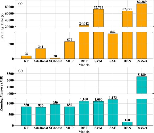
Among the nine ML models, the implementation cost for the ResNet model was the highest, with the most training time (∼24.83 h, 89,389 s) spent and the largest memory (∼5 GB, 5,280 MB) needed. For the other eight models, the time needed for model training differed greatly, with the top three being the SVM (72,723 s, ∼ 20.20 h), the DBN (67,725 s, ∼18.81 h), and the RBF (24,042 s, ∼ 6.67 h), and the least time needed was the XGBoost (28 s). The computer memory needed was similar for these models, ranging from approximately 800–1,200 MB except for the DBN, which had the least memory requirements of 160 MB. Relatively speaking, the implementation costs for the three tree methods (RF, AdaBoost and XGBoost) were the smallest, which is one of the most important reasons why the tree methods are so popular. Moreover, SVM is not suitable for large samples (Mountrakis, Im, and Ogole 2011) because it took more than 3 h for training when only 50% of the total training samples were used, which is due to the complex mapping process in SVM of the high dimensional space (Mountrakis, Im, and Ogole 2011). Therefore, the results demonstrate that the implementation costs for the DL methods are not always expensive except for ResNet, and a trade-off must be made between the running costs and model performance when selecting ML methods.

Based on the above results, it could be concluded that most DL models performed better than most traditional ML models in $R_n$ estimation, especially the ResNet model, and were followed by the SAE. However, the performance of XGBoost and MLP in the classic ML methods was also not disappointing, while RF, AdaBoost, RBF and SVM had general performances. However, the implementation cost required for the ResNet model was the highest, and some methods (e.g. SVM and RBF) worked poorly with large sample sizes.

4.3. Inter-comparison with GLASS-MODIS ${\mathit{R}}_{\mathit{n}}$ of the three outperformed models

The performance of three outperformed models, including the two DL methods, ResNet and SAE, and the one tree method, XGBoost, was further compared with the daily $R_n$ from the GLASS-MODIS product. which was thought to be much better than other existing $R_n$ products, including CERES4A (Li et al. 2021).

4.3.1. At the site scale

With the same validation samples, the validated accuracy of GLASS-MODIS $R_n$ yielded an R² of 0.87, RMSE of 24.42 Wm⁻² and bias of −1.69 Wm⁻². Combined with the results in Table 9, the outputs of the ResNet, SAE and XGBoost models were more accurate than those of GLASS-MODIS, with smaller RMSE values (19.40/20.16/20.25 Wm⁻²), biases (0.14/0.77/0.06 Wm⁻²) and larger R² values (0.92/0.91/0.91). The statistics of their validation accuracy in RMSE and bias in Figure 16 further illustrated the superiority of the three models, especially the ResNet model; hence, more comparisons between the daily $R_n$ from GLASS-MODIS and the ResNet model were conducted, and the results are shown in Figures 17 and 18.

Figure 16. The boxplot of the validation accuracy in daily ${\mathit{R}}_{\mathit{n}}$ from the GLASS-MODIS product and the ResNet, the SAE, and the XGBoost model represented by (a) bias (Wm⁻²) and (b) RMSE (Wm⁻²).

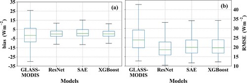
Figure 17. The performance of ResNet model and GLASS-MODIS product over twelve months in the North Hemisphere: (a) RMSE and (b) rRMSE.

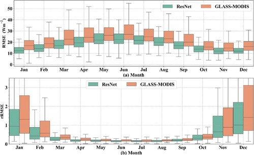
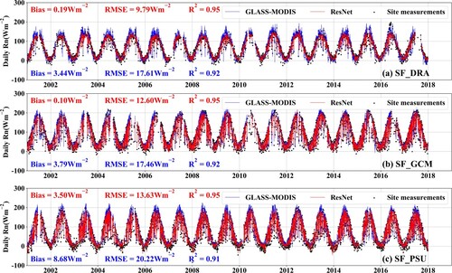
Figure 18. Time series of the estimated daily $R_n$ from ResNet model (red line), GLASS-MODIS (blue line), and in-situ measurements (black dots) at three sites: (a) SF_DRA (36.63°N, 116.02°W, BSV); (b) SF_GCM (34.25°N, 89.87°W, GRA); and (c) SF_SXF (43.73°N, 96.62°W, OSH).

Figure 17 shows the monthly validation accuracy in $R_n$ represented by RMSE (Figure 17a) and rRMSE (Figure 17b) from 2000 to 2017 in the Northern Hemisphere. It shows that the estimated $R_n$ from the ResNet model was more accurate at each of the twelve months than that of GLASS-MODIS, with smaller RMSE values ranging from 10∼26 Wm⁻² (14∼34 Wm⁻² for GLASS-MODIS) but the two both performed poorly in the cold months, which was coincident with the previous results, and this needs to be improved in the future.

To illustrate the ability to capture the temporal variations of $R_n$, the long time series daily $R_n$ estimated from the ResNet model, GLASS-MODIS, and the ground measurements were intercompared at three randomly selected SURFRAD sites (SF_DRA <36.63°N, 116.02°W, BSV>, SF_GCM <34.25°N, 89.87°W, GRA>, and SF_SXF <43.73°N, 96.62°W, OSH>) and are shown in Figure 18. It can be seen that the two daily $R_n$ estimations varied similarly to the in situ $R_n$ measurements (block dots) very well, but the variations in $R_n$ from the ResNet model (red line) were closer to the in situ one, especially at high values with a smaller overall validated RMSE (9.8∼13.6 Wm⁻²) and bias (0.1∼3.5 Wm⁻²) values than those from GLASS-MODIS (blue line). However, both of them had the tendency to overestimate the $R_n$ at very low values (∼ 0 Wm⁻²).

4.3.2. Mapping

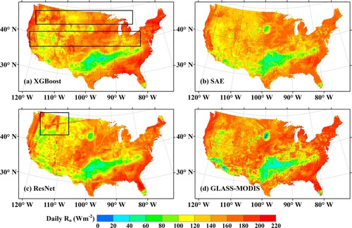
The XGBoost, SAE, and ResNet models were applied to map the daily $R_n$ over the continental United States on a randomly selected day on the 213nd day of 2017, and the results are presented in Figure 19. For reference, the GLASS-MODIS daily $R_n$ on the same day for this region is also presented (Figure 19d). Overall, the spatial distributions of the estimated daily $R_n$ from the three models (Figure 19a – c) were similar to each other and to that of GLASS-MODIS (Figure 19d). Among the three ML models, the mapping results from the SAE performed the best in regards to the spatial continuity and the production efficiency, while various issues appeared in the results of the other two models. Specifically, for the result of the XGBoost model (Figure 19a), some mosaics parallel to the latitude near ${40}^{{}^{\circ }}$N and ${45}^{{}^{\circ }}$N (black rectangle) were shown, which was speculated to be caused by taking the latitude of ${40}^{{}^{\circ }}$N and ${45}^{{}^{\circ }}$N as one of the judgement conditions, which were defined automatically in the formation of the decision trees in XGBoost, whereas for the results of the ResNet model (Figure 19c), the mosaics corresponding to the swath of the MODIS image appeared, which was possibly due to the window size (39$\times$39 km²) of the inputted active image block defined in this study, causing the calculations at the edges of the image to be invalid. In addition, the relatively large window size also made the mapped $R_n$ too smooth to provide more details compared to the others. Regarding the running time for the mapping over the continental United States for one day, it took approximately 3 days for the ResNet model and only a few hours (< 3 h) for the other two models. Hence, a reasonable trade-off between the accuracy and the running efficiency must be carefully considered when conducting global applications (Pyo et al. 2019; Jiang et al. 2020).

Figure 19. The spatial distribution of the daily ${\mathit{R}}_{\mathit{n}}$ on the 213th day of 2017 over the Continental United States from (a) the XGBoost model, (b) the SAE model, (c) the ResNet model and (d) the GLASS-MODIS product. The black boxes in (a) and (c) indicate the mosaics.

In summary, the DL methods, ResNet and SAE, outperformed most of the evaluated ML methods and the GLASS-MODIS product in daily $R_n$ estimations with a higher validation accuracy and a more robust performance under various conditions but the SAE had outstanding advantages if used for global mapping relative to ResNet because of its implementation efficiency and spatial continuity. However, the quality and quantity of the samples are still most essential to all the data-driven methods.

5. Discussion

Two more issues about the performance of the nine ML models in $R_n$ calculations need to be thoroughly discussed, including the influence of the sample size on DL methods and how these models work in predictions, especially in rugged terrain.

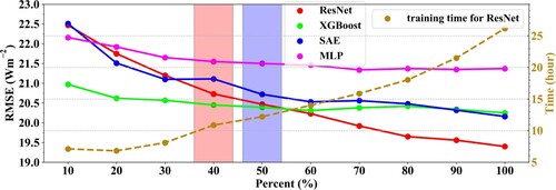
One of the issues that the users are most concerned about is the influence of the samples for model training on the performance of the DL methods, especially the influence of the sample size (Yuan et al. 2020). Hence, the validation accuracy against the same independent validation samples (No. of samples = 176,584) of the four well-performing ML models for $R_n$ estimation, including two the DL methods (ResNet and SAE) and the two classic ML methods (XGBoost and MLP), were examined with different sizes of training samples. For better illustration, the Kneed method (Satopaa et al. 2011) was applied to the four models to detect the inflection points indicating the distinct changes in the overall variations in the validated RMSE when the samples for model training increased with random selections from 10% to 100% of the overall training samples (No, of samples = 488,390) at an interval of 10%.

As Figure 20 shows, the validation accuracy for all four models generally improved with decreasing RMSE values when the training samples increased, especially for the ResNet (red dotted line) and SAE models (blue dotted line). This indicates that the performance of the two ML methods remained stable with a nearly unchanged RMSE when the employed training samples were greater than approximately 293,000 (60% of the total sample size). The performance of the two DL methods improved all the time even when all the training samples were used, especially the ResNet model, where the RMSE value decreased to 19.4 Wm⁻² but its implementation time cost for training increased significantly from 7 to 26 h. Combining the infection points detected for ResNet (red bar) and SAE (blue bar), a larger sample size was required for the DL methods, especially for ResNet, and at least 200,000 and 250,000 samples were required for the ResNet and SAE model training, respectively. However, it was still difficult to determine the best sample size for ResNet, as the validated RMSE was still decreasing when all the samples (∼500,000) were used. Therefore, by combining the model performance in $R_n$ estimations, the SAE and XGBoost methods are also good choices in addition to ResNet in practical use.

Figure 20. The variations in the validated accuracy (in RMSE, left y-axis) of the ResNet, XGBoost, SAE and MLP model for ${\mathit{R}}_{\mathit{n}}$ estimation and the implementation times (in hours, right y-axis) for the ResNet with the increased training samples. The red and blue bars represent the inflection points of the validated RMSE of the ResNet and SAE models, respectively.

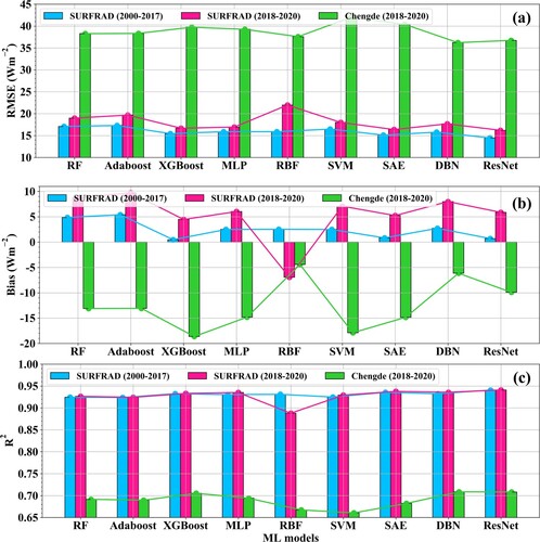
Additionally, the prediction ability of these nine ML methods in daily $R_n$ estimation was explored. The samples from 2000 to 2020 from SURFRAD with a total number of 17,962 were used for validation, in which the samples from 2000–2017 were used for validation and those from 2018–2020 were used for validating predictions. Figure 20 presents the above two results in blue bars and magenta bars for the nine ML models. Overall, the validation accuracy of the predictions from the nine models using the SURFRAD measurements is slightly worse than those from 2000 to 2017, with the RMSE values and the magnitude of bias increasing by 1∼6.1 Wm⁻² and 3.5∼5 Wm⁻², respectively. The results were still better than those for GLASS-MODIS, with RMSE values of 19.4 and 20.7 Wm⁻² and bias values of 1.4 and 6.5 Wm⁻² for 2000–2017 and 2018–2020, respectively. The short time expansion ability of the nine ML models was acceptable; hence, the nine models were used for prediction in rugged terrains. The validation results were also added in Figure 21 in green bars for all the models by using the samples from Chengde (described in Section 3.1.1). For rugged terrains, the estimation accuracy of the nine ML methods was heavily weakened as their RMSE values increased to 36∼42 Wm⁻², the magnitude of the biases was reduced by 14∼25 Wm⁻², the R² values decreased by 0.22∼0.27, and all the models had the tendency to underestimate the daily $R_n$ (negative bias). Relatively speaking, the two DL methods (DBN and ResNet) and RBF performed slightly better than the others. The data-driven methods always describe the characteristics of major samples, which is why these models performed worse in some special cases (e.g. rugged terrain). Therefore, to improve the rugged $R_n$ estimation accuracy, including more rugged terrain samples for use in for model training would be one of the solutions. In addition, the low accuracy of the rugged terrain ERA5 $R_n$ (Figure 21), which was taken as a constraint in modeling, should also be considered; therefore, further experiments have been conducted by removing the ERA5 $R_n$ in these nine models, but the estimation accuracy improved minimally. Hence, it indicated that the other constraints with higher spatial resolutions and accuracies and the parameters related to terrain both needed to be taken into account in the data-driven models for $R_n$ estimations in rugged terrain.

Figure 21. Validation accuracy of the nine ML models, GLASS-MODIS and ERA5 against the measurement from SURFRAD from 2000 to 2017 (blue) and 2018–2020 (magenta), and from Chengde at rugged terrain from 2018 to 2020 (green) in (a) RMSE (Wm⁻²), (b) bias (Wm⁻²) and (c) R².

6. Conclusions

To evaluate the performance of various ML methods in $R_n$ estimations, nine ML methods, including six classic ML methods (i.e. three tree methods, namely, RF, AdaBoost and XGBoost, two artificial neural network methods, namely, MLP and RBF, and one kernel method, namely, SVM) and three deep learning methods, namely, SAE, DBN and ResNet, were developed for estimating the daily $R_n$ at mid-low latitudes using the in situ measurements collected from 340 globally distributed sites at mid-low latitudes, MODIS TOA observations, and ERA5 $R_n$. Then, the $R_n$ estimates from the nine ML models were validated directly at the site’s scale against the same independent validation samples, and their accuracies were further examined under various conditions in terms of land cover types, elevation zones, seasons and latitudes. Finally, the estimates from the outperformed models were compared with those from the GLASS-MODIS product. The validation intercomparison results demonstrated that the three DL models, especially the ResNet and SAE models, generally outperformed all the other ML models with higher overall validation accuracies, and the XGBoost model performed the best among the six classic ML models. Specifically, the ResNet model performed the best among the nine models, yielding an overall validated RSME of 19.40 Wm⁻² and a bias of 0.14 Wm⁻², followed by the SAE and XGBoost models, which yielded validated RMSE values of 20.16 and 20.25 Wm⁻² and biases of 0.77 and 0.06 Wm⁻², respectively. In addition, the estimation accuracy of the other models was also acceptable, with RMSE values ranging from 21∼23 Wm⁻². Furthermore, the performance of the nine models across various conditions showed that the ResNet model was also the best, with the most robust performance and the highest accuracy. In addition, the accuracy of $R_n$ from ResNet, SAE, and XGBoost was better than that of the GLASS-MODIS $R_n$, whose validated RMSE was 24.42 Wm⁻² and with a bias of $-$1.69 Wm⁻². However, there were some cases under which nearly all the evaluated ML models performed unsatisfactory, such as the land cover for SAV and DNF, the elevation zones in 800∼1000 m and higher than 2000m, winter days, mid-high latitudes, and the rugged terrain. Hence, more effort should be made in the future to improve the daily $R_n$ estimation accuracy under specific cases by increasing the modeling sample size or revising the introduced modeling parameters.

Although DL methods achieved better estimation accuracies than the classic ML methods, these nine methods have their own advantages and disadvantages. For example, the DL methods represented by the ResNet and SAE models are greatly affected by the sample size, which should be large enough (> ∼200,000 and ∼250,000, respectively) to ensure the model performance but XGBoost could perform comparatively only with a much smaller sample size. Regarding the best performing ResNet, it will be difficult to apply this model for global mapping or other practical uses because of its large sample size requirements, unreasonable input window size and high implementation cost. The three tree models evaluated in this study are actually the most feasible for practical use because of their low training cost and high running efficiency. However, their accuracy was not that outstanding but it was found that discontinuous values usually appeared when using the tree methods for spatial mapping, possibly due to the discrete variables in the model inputs. For the other three classic ML or DL methods (RBF, SVM and DBN), their performance was relatively worse in $R_n$ estimations, with lower estimation accuracies and medium running efficiencies. Therefore, in terms of accuracy, running cost and mapping performance, SAE may be the best method for $R_n$ estimation, although its accuracy performance is not as high as ResNet.

Overall, this study comprehensively evaluated the performance of nine ML methods in estimating the land surface $R_n$, which could provide a good reference for other researchers. However, many novel network design methods were not considered in the present work, such as LSTM (Ghimire 2019), spatiotemporal weighted neural networks (Li et al. 2020), and generative adversarial networks (GANs) (Hayatbini et al. 2019); hence, additional work needs to be conducted in the future.

Authorship contribution statement

Shaopeng Li: Conceptualization, Investigation, Methodology, Software, Data curation, Visualization, Writing – original draft. Bo Jiang: Methodology, Resources, Investigation, Data curation, Writing – review & editing, Funding acquisition. Shunlin Liang: Methodology, Investigation, Supervision. Jianghai Peng, Hui Liang, Jiakun Han and Xiuwan Yin: Data curation, Supervision. Yunjun Yao, Xiaotong Zhang, Jie Cheng, Xiang Zhao, Qiang Liu and Kun Jia: Supervision.

Data availability

We appreciate the radiation measurements provided by the FLUXNET community, in particular by the following networks: AmeriFlux (U.S. Department of Energy, Biological and Environmental Research, Terrestrial Carbon Program (DE-FG02-04ER63917)), AfriFlux, AsiaFlux, CarboAfrica, CarboEuropeIP, CarboItaly, CarboMont, ChinaFlux, Fluxnet- Canada (supported by CFCAS, NSERC, BIOCAP, Environment Canada, and NRCan), GreenGrass, KoFlux, LBA, NECC, OzFlux, TCOS-Siberia, USCCC. Additionally, we are thankful for the Chengde dataset provided by the Chengde Remote Sensing Test Site, State Key Laboratory of Remote Sensing Sciences. The authors acknowledge the financial support for the eddy covariance data harmonization provided by CarboEuropeIP, FAO-GTOS-TCO, Ileaps, Max Planck Institute for Biogeochemistry, National Science Foundation, University of Tuscia, Université Laval, Environment Canada and the US Department of Energy and the dataset development and technical support from the Berkeley Water Center, Lawrence Berkeley National Laboratory, Microsoft Research Science, Oak Ridge National Laboratory, University of California—Berkeley and the University of Virginia. The authors would also like to thank other radiation measurement providers (listed in Table 1).

Disclosure statement

No potential conflict of interest was reported by the author(s).

Additional information

Funding

This work was supported by National Natural Science Foundation of China: [grant no 41971291, 42090012]; National Key Research and Development Program of China: [grant no 2020YFA0608704].

References

- Aghdam, H. H., and E. J. Heravi. 2017. Guide to Convolutional Neural Networks. New York, NY: Springer 10(978-973), 51.
- Ağbulut, Ü, A. E. Gürel, and Y. Biçen. 2021. “Prediction of Daily Global Solar Radiation Using Different Machine Learning Algorithms: Evaluation and Comparison.” Renewable and Sustainable Energy Reviews 135: 110114.
- Alados, I., I. Foyo-Moreno, F. J. Olmo, and L. Alados-Arboledas. 2003. “Relationship Between net Radiation and Solar Radiation for Semi-Arid Shrub-Land.” Agricultural and Forest Meteorology 116 (3): 221–227.
- Amit, Y., and D. Geman. 1997. “Shape Quantization and Recognition with Randomized Trees.” Neural Computation 9: 1545–1588.
- Augustine, J. A., J. J. DeLuisi, and C. N. Long. 2000. “SURFRAD—A National Surface Radiation Budget Network for Atmospheric Research.” Bulletin of the American Meteorological Society 81: 2341–2357.
- Behrang, M., E. Assareh, A. Ghanbarzadeh, and A. Noghrehabadi. 2010. “The Potential of Different Artificial Neural Network (ANN) Techniques in Daily Global Solar Radiation Modeling Based on Meteorological Data.” Solar Energy 84 (8): 1468–1480.
- Bengio, Y., A. Courville, and P. Vincent. 2013. “Representation Learning: A Review and New Perspectives.” IEEE Transactions on Pattern Analysis and Machine Intelligence 35 (8): 1798–1828.
- Bishop, C. M. 1995. Neural Networks for Pattern Recognition. New York: Oxford university press.
- Bisht, G., and R. L. Bras. 2010. “Estimation of Net Radiation from the MODIS Data Under all Sky Conditions: Southern Great Plains Case Study.” Remote Sensing of Environment 114 (7): 1522–1534.
- Bisht, G., V. Venturini, S. Islam, and L. Jiang. 2005. “Estimation of the Net Radiation Using MODIS (Moderate Resolution Imaging Spectroradiometer) Data for Clear Sky Days.” Remote Sensing of Environment 97 (1): 52–67.
- Breiman, L. 1996. “Bagging Predictors.” Machine Learning 24 (2): 123–140.
- Broomhead, D. S., and D. Lowe. 1988. “Multivariable Functional Interpolation and Adaptive Networks.” Complex System 2: 321–355.
- Brown, M. G. L., S. Skakun, T. He, and S. Liang. 2020. “Intercomparison of Machine-Learning Methods for Estimating Surface Shortwave and Photosynthetically Active Radiation.” Remote Sensing 12 (3): 372.
- Carmona, F., R. Rivas, and V. Caselles. 2015. “Development of a General Model to Estimate the Instantaneous, Daily, and Daytime Net Radiation with Satellite Data on Clear-Sky Days.” Remote Sensing of Environment 171: 1–13.
- Carter, C., and S. Liang. 2019. “Evaluation of Ten Machine Learning Methods for Estimating Terrestrial Evapotranspiration from Remote Sensing.” International Journal of Applied Earth Observation and Geoinformation 78: 86–92.
- Chen, X., G. de Leeuw, A. Arola, S. Liu, Y. Liu, Z. Li, and K. Zhang. 2020. “Joint Retrieval of the Aerosol Fine Mode Fraction and Optical Depth Using MODIS Spectral Reflectance Over Northern and Eastern China: Artificial Neural Network Method.” Remote Sensing of Environment 249: 112006.
- Chen, T., and C. Guestrin. 2016. “XGBoost: A Scalable Tree Boosting System.” Proceedings of the 22nd ACM SIGKDD International Conference on Knowledge Discovery and Data Mining. San Francisco, California, USA, Association for Computing Machinery: 785–794.
- Chen, J., T. He, B. Jiang, and S. Liang. 2020. “Estimation of All-Sky All-Wave Daily Net Radiation at High Latitudes from MODIS Data.” Remote Sensing of Environment 245: 111842.
- Chen, J.-L., G.-S. Li, and S. Wu. 2013. “Assessing the Potential of Support Vector Machine for Estimating Daily Solar Radiation Using Sunshine Duration.” Energy Conversion and Management 75: 311–318.
- da Silva, B. B., S. M. G. L. Montenegro, V. D. P. R. da Silva, H. R. da Rocha, J. D. Galvíncio, and L. M. M. de Oliveira. 2015. “Determination of Instantaneous and Daily Net Radiation from TM – Landsat 5 Data in a Subtropical Watershed.” Journal of Atmospheric and Solar-Terrestrial Physics 135: 42–49.
- Dee, D. P., S. M. Uppala, A. J. Simmons, P. Berrisford, P. Poli, S. Kobayashi, U. Andrae, et al. 2011. “The ERA-Interim Reanalysis: Configuration and Performance of the Data Assimilation System.” Quarterly Journal of the Royal Meteorological Society 137 (656): 553–597.
- Dietterich, T. G. 2000. “An Experimental Comparison of Three Methods for Constructing Ensembles of Decision Trees: Bagging, Boosting, and Randomization.” Machine Learning 40 (2): 139–157.
- Fan, J., X. Wang, L. Wu, H. Zhou, F. Zhang, X. Yu, X. Lu, and Y. Xiang. 2018. “Comparison of Support Vector Machine and Extreme Gradient Boosting for Predicting Daily Global Solar Radiation Using Temperature and Precipitation in Humid Subtropical Climates: A Case Study in China.” Energy Conversion and Management 164: 102–111.
- Fan, J., L. Wu, F. Zhang, H. Cai, W. Zeng, X. Wang, and H. Zou. 2019. “Empirical and Machine Learning Models for Predicting Daily Global Solar Radiation from Sunshine Duration: A Review and Case Study in China.” Renewable and Sustainable Energy Reviews 100: 186–212.
- Fan, J., J. Zheng, L. Wu, and F. Zhang. 2021. “Estimation of Daily Maize Transpiration Using Support Vector Machines, Extreme Gradient Boosting, Artificial and Deep Neural Networks Models.” Agricultural Water Management 245: 106547.
- Feng, Y., W. Hao, H. Li, N. Cui, D. Gong, and L. Gao. 2020. “Machine Learning Models to Quantify and map Daily Global Solar Radiation and Photovoltaic Power.” Renewable and Sustainable Energy Reviews 118: 109393.
- Ferreira, A. G., E. Soria-Olivas, A. J. S. López, E. J. T. López-Baeza, and A. Climatology. 2011. “Estimating NET Radiation at Surface Using Artificial Neural Networks: A New Approach.” Theoretical and Applied Climatology 106: 263–279.
- Freund, Y., and R. E. Schapire. 1997. “A Decision-Theoretic Generalization of On-Line Learning and an Application to Boosting.” Journal of Computer and System Sciences 55 (1): 119–139.
- Fu, B., S. Li, X. Yu, P. Yang, G. Yu, R. Feng, and X. Zhuang. 2010. “Chinese Ecosystem Research Network: Progress and Perspectives.” Ecological Complexity 7 (2): 225–233.
- Ge, L., R. Hang, Y. Liu, and Q. Liu. 2018. “Comparing the Performance of Neural Network and Deep Convolutional Neural Network in Estimating Soil Moisture from Satellite Observations.” Remote Sensing 10 (9): 1327.
- Ghimire, S. 2019. “Deep Solar Radiation Forecasting with Convolutional Neural Network and Long Short-Term Memory Network Algorithms.” Applied Energy 253: 113541.
- Gislason, P. O., J. A. Benediktsson, and J. R. Sveinsson. 2006. “Random Forests for Land Cover Classification.” Pattern Recognition Letters 27 (4): 294–300.
- Guo, L., P.-S. Ge, M.-H. Zhang, L.-H. Li, and Y.-B. Zhao. 2012. “Pedestrian Detection for Intelligent Transportation Systems Combining AdaBoost Algorithm and Support Vector Machine.” Expert Systems with Applications 39 (4): 4274–4286.
- Guo, X., Y. Yao, Y. Zhang, Y. Lin, B. Jiang, K. Jia, X. Zhang, et al. 2020. “Discrepancies in the Simulated Global Terrestrial Latent Heat Flux from GLASS and MERRA-2 Surface Net Radiation Products.” Remote Sensing 12 (17): 2763.
- Hassan, M., A. Khalil, S. Kaseb, and M. A. Kassem. 2017. “Exploring the Potential of Tree-Based Ensemble Methods in Solar Radiation Modeling.” Applied Energy 203: 897–916.
- Hayatbini, N., B. Kong, K. L. Hsu, P. Nguyen, S. Sorooshian, G. Stephens, C. Fowlkes, R. Nemani, and S. Ganguly. 2019. “Conditional Generative Adversarial Networks (cGANs) for Near Real-Time Precipitation Estimation from Multispectral GOES-16 Satellite Imageries—PERSIANN-cGAN.” Remote Sensing 11 (19): 2193.
- He, K., X. Zhang, S. Ren, and J. Sun. 2016. “Deep Residual Learning for Image Recognition.” Proceedings of the IEEE Conference on Computer Vision and Pattern Recognition.
- Hersbach, H., B. Bell, P. Berrisford, S. Hirahara, A. Horányi, J. Muñoz-Sabater, J. Nicolas, et al. 2020. “The ERA5 Global Reanalysis.” Quarterly Journal of the Royal Meteorological Society 146 (730): 1999–2049.
- Hinton, G. E., S. Osindero, and Y.-W. Teh. 2006. “A Fast Learning Algorithm for Deep Belief Nets.” Neural Computation 18 (7): 1527–1554.
- Hochreiter, S., and J. Schmidhuber. 1997. “Long Short-Term Memory.” Neural Computation 9 (8): 1735–1780.
- Hou, N., X. Zhang, W. Zhang, Y. Wei, K. Jia, Y. Yao, B. Jiang, and J. Cheng. 2020. “Estimation of Surface Downward Shortwave Radiation Over China from Himawari-8 ahi Data Based on Random Forest.” Remote Sensing 12 (1): 181.
- Huang, G., C. Huang, L. Shaomin, Y. Ma, and H. Chen. 2016. “Representativeness Errors of Point-Scale Ground-Based Solar Radiation Measurements in the Validation of Remote Sensing Products.” Remote Sensing of Environment 181: 198–206.
- Ibrahim, I. A., and T. Khatib. 2017. “A Novel Hybrid Model for Hourly Global Solar Radiation Prediction Using Random Forests Technique and Firefly Algorithm.” Energy Conversion and Management 138: 413–425.
- Ioffe, S., and C. Szegedy. 2015. “Batch Normalization: Accelerating Deep Network Training by Reducing Internal Covariate Shift.” Proceedings of the 32nd International Conference on International Conference on Machine Learning - Volume 37. Lille, France, JMLR.org.
- Jafarzadeh, H., M. Mahdianpari, E. Gill, F. Mohammadimanesh, and S. Homayouni. 2021. “Bagging and Boosting Ensemble Classifiers for Classification of Multispectral, Hyperspectral and PolSAR Data: A Comparative Evaluation.” Remote Sensing 13 (21): 4405.
- Jiang, B., S. Liang, H. Ma, X. Zhang, Z. Xiao, X. Zhao, K. Jia, Y. Yao, and A. Jia. 2016. “GLASS Daytime All-Wave Net Radiation Product: Algorithm Development and Preliminary Validation.” Remote Sensing 8 (3): 222.
- Jiang, H., N. Lu, G. Huang, L. Yao, J. Qin, and H. Liu. 2020. “Spatial Scale Effects on Retrieval Accuracy of Surface Solar Radiation Using Satellite Data.” Applied Energy 270: 115178.
- Jiang, H., N. Lu, J. Qin, W. Tang, and L. Yao. 2019. “A Deep Learning Algorithm to Estimate Hourly Global Solar Radiation from Geostationary Satellite Data.” Renewable and Sustainable Energy Reviews 114: 109327.
- Jiang, B., Y. Zhang, S. Liang, X. Zhang, and Z. Xiao. 2014. “Surface Daytime Net Radiation Estimation Using Artificial Neural Networks.” Remote Sensing 6 (11): 11031–11050.
- Kim, H.-Y., and S. Liang. 2010. “Development of a Hybrid Method for Estimating Land Surface Shortwave Net Radiation from MODIS Data.” Remote Sensing of Environment 114 (11): 2393–2402.
- Kingma, D., and J. Ba. 2014. “Adam: A Method for Stochastic Optimization.” International conference on learning representations.
- Kisi, O., M. Alizamir, S. Trajkovic, J. Shiri, and S. Kim. 2020. “Solar Radiation Estimation in Mediterranean Climate by Weather Variables Using a Novel Bayesian Model Averaging and Machine Learning Methods.” Neural Processing Letters 52 (3): 2297–2318.
- Kratz, D. P., S. K. Gupta, A. C. Wilber, and V. E. Sothcott. 2020. “Validation of the CERES Edition-4A Surface-Only Flux Algorithms.” Journal of Applied Meteorology and Climatology 59 (2): 281–295.
- Krizhevsky, A., I. Sutskever, and G. E. Hinton. 2012. “ImageNet Classification with Deep Convolutional Neural Networks.” Proceedings of the 25th International Conference on Neural Information Processing Systems - Volume 1. Lake Tahoe, NEVADA, Curran Associates Inc. 1097–1105.
- Kussul, N., M. Lavreniuk, S. Skakun, and A. Shelestov. 2017. “Deep Learning Classification of Land Cover and Crop Types Using Remote Sensing Data.” IEEE Geoscience and Remote Sensing Letters 14 (5): 778–782.
- LeCun, Y., Y. Bengio, and G. Hinton. 2015. “Deep Learning.” Nature 521 (7553): 436–444.
- Li, Z., M. C. Cribb, F.-L. Chang, A. Trishchenko, and Y. Luo. 2005. “Natural Variability and Sampling Errors in Solar Radiation Measurements for Model Validation Over the Atmospheric Radiation Measurement Southern Great Plains Region.” Journal of Geophysical Research: Atmospheres 110 (D15): S19.
- Li, S., B. Jiang, J. Peng, H. Liang, J. Han, Y. Yao, X. Zhang, et al. 2021. “Estimation of the All-Wave All-Sky Land Surface Daily Net Radiation at Mid-Low Latitudes from MODIS Data Based on ERA5 Constraints.” Remote Sensing 14 (1): 33.
- Li, T., H. Shen, Q. Yuan, and L. Zhang. 2020. “Geographically and Temporally Weighted Neural Networks for Satellite-Based Mapping of Ground-Level PM2.5.” ISPRS Journal of Photogrammetry and Remote Sensing 167: 178–188.
- Li, T., H. Shen, Q. Yuan, X. Zhang, and L. Zhang. 2017. “Estimating Ground-Level PM2.5 by Fusing Satellite and Station Observations: A Geo-Intelligent Deep Learning Approach.” Geophysical Research Letters 44 (23): 11,985–11,993.
- Liang, S., J. Cheng, K. Jia, B. Jiang, Q. Liu, Z. Xiao, Y. Yao, et al. 2021. “The Global Land Surface Satellite (GLASS) Product Suite.” Bulletin of the American Meteorological Society 102 (2): E323–E337.
- Liang, S., K. Wang, X. Zhang, and M. Wild. 2010. “Review on Estimation of Land Surface Radiation and Energy Budgets from Ground Measurement, Remote Sensing and Model Simulations.” IEEE Journal of Selected Topics in Applied Earth Observations and Remote Sensing 3 (3): 225–240.
- Lim, B., S. Son, H. Kim, S. Nah, and K. M. Lee. 2017. Enhanced Deep Residual Networks for Single Image Super-Resolution.
- Loveland, T. R., and A. S. Belward. 1997. “The IGBP-DIS Global 1km Land Cover Data set, DISCover: First Results.” International Journal of Remote Sensing 18 (15): 3289–3295.
- Martens, B., D. L. Schumacher, H. Wouters, J. Muñoz-Sabater, N. E. Verhoest, and D. G. Miralles. 2020. “Evaluating the Land-Surface Energy Partitioning in ERA5.” Geoscientific Model Development 13 (9): 4159–4181.
- Mas, J. F., and J. J. Flores. 2008. “The Application of Artificial Neural Networks to the Analysis of Remotely Sensed Data.” International Journal of Remote Sensing 29 (3): 617–663.
- Min, M., J. Li, F. Wang, Z. Liu, and W. P. Menzel. 2020. “Retrieval of Cloud top Properties from Advanced Geostationary Satellite Imager Measurements Based on Machine Learning Algorithms.” Remote Sensing of Environment 239: 111616.
- Mountrakis, G., J. Im, and C. Ogole. 2011. “Support Vector Machines in Remote Sensing: A Review.” ISPRS Journal of Photogrammetry and Remote Sensing 66 (3): 247–259.
- Nair, V., and G. E. Hinton. 2010. “Rectified Linear Units Improve Restricted Boltzmann Machines.” Proceedings of the 27th International Conference on International Conference on Machine Learning. Haifa, Israel, Omnipress, 807–814.
- Ornl, D. 2015. “FLUXNET Web Page. Retrieved from http://fluxnet.ornl.gov.”.
- Pedregosa, F., G. Varoquaux, A. Gramfort, V. Michel, B. Thirion, O. Grisel, M. Blondel, et al. 2011. “Scikit-learn: Machine Learning in Python.” The Journal of Machine Learning Research 12: 2825–2830.
- Peel, M. C., B. L. Finlayson, and T. A. McMahon. 2007. “Updated World map of the Köppen-Geiger Climate Classification.” Hydrology and Earth System Sciences 11 (5): 1633–1644.
- Phillips, T. J., S. A. Klein, H. Y. Ma, Q. Tang, S. Xie, I. N. Williams, J. A. Santanello, D. R. Cook, and M. S. Torn. 2017. “Using ARM Observations to Evaluate Climate Model Simulations of Land-Atmosphere Coupling on the U.S. Southern Great Plains.” Journal of Geophysical Research: Atmospheres 122 (21): 11,524–11,548.
- Pyo, J., H. Duan, S. Baek, M. S. Kim, T. Jeon, Y. S. Kwon, H. Lee, and K. H. Cho. 2019. “A Convolutional Neural Network Regression for Quantifying Cyanobacteria Using Hyperspectral Imagery.” Remote Sensing of Environment 233: 111350.
- Romanuke, V. 2017. Appropriate Number and Allocation of RELUS in Convolutional Neural Networks.” Research Bulletin of the National Technical University of Ukraine Kyiv Politechnic Institute: 69-78.
- Sain, S. R. 1996. “The Nature of Statistical Learning Theory.” Taylor & Francis 38: 409–409.
- Satopaa, V., J. Albrecht, D. Irwin, and B. Raghavan. 2011. “Finding a “Kneedle” in a Haystack: Detecting Knee Points in System Behavior.” 2011 31st International Conference on Distributed Computing Systems Workshops.
- Shaomin, L., M. Ma, Q. Xiao, Q. Liu, R. Jin, et al. 2012. “HiWATER: An Integrated Remote Sensing Experiment on Hydrological and Ecological Processes in the Heihe River Basin.” Chinese Journal 27: 481–498.
- Shen, H., Y. Jiang, T. Li, Q. Cheng, C. Zeng, and L. Zhang. 2020. “Deep Learning-Based air Temperature Mapping by Fusing Remote Sensing, Station, Simulation and Socioeconomic Data.” Remote Sensing of Environment 240: 111692.
- Shen, H., T. Li, Q. Yuan, and L. Zhang. 2018. “Estimating Regional Ground-Level PM2.5 Directly from Satellite Top-of-Atmosphere Reflectance Using Deep Belief Networks.” Journal of Geophysical Research: Atmospheres 123 (24): 13,875–13,886.
- Shi, Q., and S. Liang. 2013. “Characterizing the Surface Radiation Budget Over the Tibetan Plateau with Ground-Measured, Reanalysis, and Remote Sensing Data Sets: 2. Spatiotemporal Analysis.” Journal of Geophysical Research: Atmospheres 118 (16): 8921–8934.
- Sianturi, Y., and S. Marjuki Kwarti. 2020. “Evaluation of ERA5 and MERRA2 Reanalyses to Estimate Solar Irradiance Using Ground Observations Over Indonesia Region.” American institute of physics conference series.
- Swap, R. J., H. J. Annegarn, J. T. Suttles, M. D. King, S. Platnick, J. L. Privette, and R. J. Scholes. 2003. “Africa Burning: A Thematic Analysis of the Southern African Regional Science Initiative (SAFARI 2000).” Journal of Geophysical Research: Atmospheres 108 (D13): 8465.
- Tan, J., N. NourEldeen, K. Mao, J. Shi, Z. Li, T. Xu, and Z. Yuan. 2019. “Deep Learning Convolutional Neural Network for the Retrieval of Land Surface Temperature from AMSR2 Data in China.” Sensors 19 (13): 2987.
- Thongkam, J., G. Xu, and Y. Zhang. 2008. “AdaBoost Algorithm with Random Forests for Predicting Breast Cancer Survivability.” 2008 Ieee International Joint Conference on Neural Networks (IEEE World Congress on Computational Intelligence).
- Tóta, J., D. R. Fitzjarrald, R. M. Staebler, R. K. Sakai, O. M. Moraes, O. C. Acevedo, S. C. Wofsy, and A. O. Manzi. 2008. “Amazon Rain Forest Subcanopy Flow and the Carbon Budget: Santarém LBA-ECO Site.” Journal of Geophysical Research: Biogeosciences 113: 1–16.
- Tsai, C., Y. Chih, W. H. Wong, and C. Lee. 2015. “A Hardware-Efficient Sigmoid Function With Adjustable Precision for a Neural Network System.” IEEE Transactions on Circuits and Systems II: Express Briefs 62 (11): 1073–1077.
- Verma, M., J. B. Fisher, K. Mallick, Y. Ryu, H. Kobayashi, A. Guillaume, G. Moore, et al. 2016. “Global Surface Net-Radiation at 5 km from MODIS Terra.” Remote Sensing 8 (9): 739.
- Wang, Y., B. Jiang, S. Liang, D. Wang, T. He, Q. Wang, X. Zhao, and J. Xu. 2019. “Surface Shortwave Net Radiation Estimation from Landsat TM/ETM+ Data Using Four Machine Learning Algorithms.” Remote Sensing 11 (23): 2847.
- Wang, D., S. Liang, T. He, and Q. Shi. 2015a. “Estimating Clear-sky all-Wave net Radiation from Combined Visible and Shortwave Infrared (VSWIR) and Thermal Infrared (TIR) Remote Sensing Data.” Remote Sensing of Environment 167: 31–39.
- Wang, D., S. Liang, T. He, and Q. Shi. 2015b. “Estimation of Daily Surface Shortwave Net Radiation from the Combined MODIS Data.” IEEE Transactions on Geoscience and Remote Sensing 53 (10): 5519–5529.
- Wang, X., and H. Liu. 2018. “Soft Sensor Based on Stacked Auto-Encoder Deep Neural Network for air Preheater Rotor Deformation Prediction.” Advanced Engineering Informatics 36: 112–119.
- Wang, Y., and H. Xu. 2005. “Spectral Characterization of Scanner Based on PCA and BP ANN.” Chinese Optics Letters 3 (12): 725–728.
- Wang, D., J. Zeng, and S. B. Lin. 2021. “Random Sketching for Neural Networks With ReLU.” IEEE Transactions on Neural Networks and Learning Systems 32 (2): 748–762.
- Wang, S., J. Zhou, T. Lei, H. Wu, X. Zhang, J. Ma, and H. Zhong. 2020. “Estimating Land Surface Temperature from Satellite Passive Microwave Observations with the Traditional Neural Network, Deep Belief Network, and Convolutional Neural Network.” Remote Sensing 12 (17): 2691.
- Wei, Y., X. Zhang, N. Hou, W. Zhang, K. Jia, and Y. Yao. 2019. “Estimation of Surface Downward Shortwave Radiation Over China from AVHRR Data Based on Four Machine Learning Methods.” Solar Energy 177: 32–46.
- Wu, P., Z. Yin, H. Yang, Y. Wu, and X. Ma. 2019. “Reconstructing Geostationary Satellite Land Surface Temperature Imagery Based on a Multiscale Feature Connected Convolutional Neural Network.” Remote Sensing 11 (3): 300.
- Wu, H., and W. Ying. 2019. “Benchmarking Machine Learning Algorithms for Instantaneous Net Surface Shortwave Radiation Retrieval Using Remote Sensing Data.” Remote Sensing 11 (21): 2520.
- Xu, J., B. Jiang, S. Liang, X. Li, Y. Wang, J. Peng, H. Chen, H. Liang, and S. Li. 2021. “Generating a High-Resolution Time-Series Ocean Surface Net Radiation Product by Downscaling J-OFURO3.” IEEE Transactions on Geoscience and Remote Sensing 59 (4): 2794–2809.
- Xu, J., S. Liang, and B. Jiang. 2022. “A Global Long-Term (1981–2019) Daily Land Surface Radiation Budget Product from AVHRR Satellite Data Using a Residual Convolutional Neural Network.” Earth System Science Data 14 (5): 2315–2341.
- Xue, M., R. Hang, Q. Liu, X.-T. Yuan, and X. Lu. 2021. “CNN-based Near-Real-Time Precipitation Estimation from Fengyun-2 Satellite Over Xinjiang, China.” Atmospheric Research 250: 105337.
- Yan, G., Q. Chu, Y. Tong, X. Mu, J. Qi, Y. Zhou, Y. Liu, et al. 2020a. “An Operational Method for Validating the Downward Shortwave Radiation Over Rugged Terrains.” IEEE Transactions on Geoscience and Remote Sensing 59 (1): 714–731.
- Yan, G., Z.-H. Jiao, T. Wang, and X. Mu. 2020b. “Modeling Surface Longwave Radiation Over High-Relief Terrain.” Remote Sensing of Environment 237: 111556.
- Yan, G., Y. Tong, K. Yan, X. Mu, Q. Chu, Y. Zhou, Y. Liu, et al. 2018. “Temporal Extrapolation of Daily Downward Shortwave Radiation Over Cloud-Free Rugged Terrains. Part 1: Analysis of Topographic Effects.” IEEE Transactions on Geoscience and Remote Sensing 56 (11): 6375–6394.
- Yao, Y., S. Liang, X. Li, J. Chen, K. Wang, K. Jia, J. Cheng, et al. 2014. “Bayesian Multimodel Estimation of Global Terrestrial Latent Heat Flux from Eddy Covariance, Meteorological, and Satellite Observations.” Journal of Geophysical Research: Atmospheres 119 (8): 4521–4545.
- Yao, Y., S. Liang, X. Li, J. Chen, K. Wang, K. Jia, J. Cheng, et al. 2015. “A Satellite-Based Hybrid Algorithm to Determine the Priestley–Taylor Parameter for Global Terrestrial Latent Heat Flux Estimation Across Multiple Biomes.” Remote Sensing of Environment 165: 216–233.
- Yeom, J.-M., S. Park, T. Chae, J.-Y. Kim, and C. S. Lee. 2019. “Spatial Assessment of Solar Radiation by Machine Learning and Deep Neural Network Models Using Data Provided by the COMS MI Geostationary Satellite: A Case Study in South Korea.” Sensors 19: 2082.
- Yuan, Q., H. Shen, T. Li, Z. Li, S. Li, Y. Jiang, H. Xu, et al. 2020. “Deep Learning in Environmental Remote Sensing: Achievements and Challenges.” Remote Sensing of Environment 241: 111716.
- Yuchechen, A. E., S. G. Lakkis, A. Caferri, P. O. Canziani, and J. P. Muszkats. 2020. “A Cluster Approach to Cloud Cover Classification Over South America and Adjacent Oceans Using a k-Means/k-Means++ Unsupervised Algorithm on GOES IR Imagery.” Remote Sensing 12: 2991.
- Zang, H., L. Cheng, T. Ding, K. W. Cheung, M. Wang, Z. Wei, and G. Sun. 2020. “Application of Functional Deep Belief Network for Estimating Daily Global Solar Radiation: A Case Study in China.” Energy 191: 116502.
- Zhang, S., H. Gao, and Y. Song. 2016a. “A New Fault-Location Algorithm for Extra-High-Voltage Mixed Lines Based on Phase Characteristics of the Hyperbolic Tangent Function.” IEEE Transactions on Power Delivery 31 (3): 1203–1212.
- Zhang, L., L. Zhang, and B. Du. 2016b. “Deep Learning for Remote Sensing Data: A Technical Tutorial on the State of the Art.” IEEE Geoscience and Remote Sensing Magazine 4 (2): 22–40.
- Zhang, B., H. Zhang, G. Zhao, and J. Lian. 2020. “Constructing a PM2.5 Concentration Prediction Model by Combining Auto-Encoder with Bi-LSTM Neural Networks.” Environmental Modelling & Software 124: 104600.
- Zo, I.-S., J.-B. Jee, B.-Y. Kim, and K.-T. Lee. 2017. “Baseline Surface Radiation Network (BSRN) Quality Control of Solar Radiation Data on the Gangneung-Wonju National University Radiation Station.” Asia-Pacific Journal of Atmospheric Sciences 53: 11–19.