Operational continental-scale land cover mapping of Australia using the Open Data Cube

ABSTRACT

To comprehensively support national and international initiatives for sustainable development, land cover products need to be reliably and routinely generated within operational frameworks. Coupled with consistent semantics and taxonomies, ensuring confidence in mapping land cover for multiple time periods, facilitates informed decision-making at scales appropriate to multiple policy domains. The United Nations Food and Agriculture Organisation (FAO) Land Cover Classification System (LCCS) provides a taxonomy that comparable at different scales, level of detail and geographic location. The Open Data Cube (ODC) initiative offers a framework for operational continental-scale land cover mapping using analysis-ready Earth Observation data. This study utilised the FAO LCCS framework and the Landsat sensor data through Digital Earth Australia (DEA; Australia’s ODC instance) to generate consistent and continent-wide land cover mapping (DEA Land Cover) of the Australian continent. DEA Land Cover provides annual maps from 1988 to 2020 at 25 m resolution. Output maps were validated with ∼12,000 independent validation points, giving an overall map accuracy of 80%. DEA Land Cover provides Australia with a nationally consistent picture of land cover, with an open-source software package using readily available global coverage data and demonstrates a pathway of adoption for national implementations across the world.

KEYWORDS:

• DEA land cover
• digital earth Australia
• FAO LCCS
• landsat
• sustainable development goals

1. Introduction

Identifying the state and condition of landscapes through continuous monitoring is paramount to ecological sustainable development (Díaz et al. 2019). This is becoming increasingly urgent given the rapid changes occurring globally in relation to declared climate and biodiversity emergencies (Tollefson 2019; Gills and Morgan 2020). Landscape state can be identified using land cover, an effective and easily interpretable biophysical descriptor of the Earth’s surface (Wulder et al. 2018). Earth Observation (EO) can provide spatially and temporally explicit land cover information, identifying landscape state and its change over time and space. Reliable, standardised, continental-scale mapping of land cover facilitates informed decision-making at scales appropriate for planning and implementing national and international policies on sustainable development (Franklin and Wulder 2002; Kavvada et al. 2020; Metternicht, Mueller, and Lucas 2020; Mohamed-Ghouse et al. 2021). The provision of ongoing and reproducible land cover maps, particularly at high spatial and temporal scales, has been difficult to achieve in the past (Grekousis, Mountrakis, and Kavouras 2015; Gómez, White, and Wulder 2016). Recent efforts in analysis-ready data (ARD) accessibility and advances in systems capable of providing computational requirements are timely to address these challenges, whereby demand for land cover maps intersects current capacity to provide products that meet end user requirements (Wulder et al. 2018; Homer et al. 2020).

Land cover maps generated recently have overcome several historical limitations of mapping at national and continental scales. Contemporary efforts mapping land cover for Europe (Pflugmacher et al. 2019; Malinowski et al. 2020; Venter and Sydenham 2021), China (Yang and Huang 2021), Africa (Li et al. 2020; Zhang et al. 2020), the conterminous United States (Homer et al. 2020), and near-real time global land use land cover (Brown et al. 2022) have generated products at greater spatial resolutions (i.e. 10 m using Sentinel-2, 30 m using Landsat-8) and higher temporal frequencies (e.g. updated map every 1–5 years), providing valuable data for identifying large scale landscape change. However, the transferability of methods and land cover taxonomies remains a common limitation to widespread adoption beyond the geographic extent or particular year of method development. Several methods use disaggregation measures or ancillary data to account for climatic variation (Pflugmacher et al. 2019; Venter and Sydenham 2021), or employ numerous spatially-stratified models to ensure high classification accuracy of the end mapping product (Inglada et al. 2017; Zhang et al. 2020). Similarly, selected land cover taxonomies are often relevant to a limited geographic extent (Griffiths, Nendel, and Hostert 2019; Ghorbanian et al. 2020), or reflect a data-driven approach (e.g. based on reference data available) (Li et al. 2020; Malinowski et al. 2020; Brown et al. 2022), where land cover classes may not be applicable for many end user requirements (e.g. supporting regional and national policy implementation).

The increasing need to monitoring landscape change for sustainable development, as well as identifying opportunities for climate change mitigation and adaptation, ecosystem restoration and biodiversity conservation, requires ongoing and routine generation of land cover products (Metternicht, Mueller, and Lucas 2020; Owers et al. 2021). National and international efforts to report landscape change, such as the United Nations System of Environmental Economic Accounting (SEEA) and Sustainable Development Goals (SDGs), rely on consistent and relevant national to global land cover information (Kavvada et al. 2020; Metternicht, Mueller, and Lucas 2020; Skidmore et al. 2021). However, many existing products are unsuitable for this reporting as they are not produced routinely or on a consistent, long-term basis, providing only a snapshot of landscape state for specific years (Griffiths, Nendel, and Hostert 2019; Venter and Sydenham 2021). Often methods applied in previous iterations vary widely (e.g. Li et al. 2020; Zhang et al. 2020), requiring modifications for additional retrieval and generation of updated maps (e.g. changing land cover semantics and taxonomy, updated machine learning algorithms). Such variations in the production of land cover information make comparisons between maps through time very difficult (Herold et al. 2016; Phiri and Morgenroth 2017; Yang et al. 2017), limiting confidence in their use for identifying changes in landscape states.

Australia, a country with diverse and dynamic landscapes, is a prime example of the essential need for routine mapping and monitoring of landscape state. To date, the National Dynamic Land Cover Dataset (DLCD) (Lymburner et al. 2011) has provided a nationally consistent land cover product for Australia and its territories (2002–2015). However, the maps are limited in their capacity to identify landscape change, largely because these were produced from a 250 m resolution MODIS composite product encompassing multiple years. Recent advances have utilised the DLCD within a machine learning approach to achieve 30 m resolution mapping for 5-year epochs based on Landsat sensor data (Calderón-Loor, Hadjikakou, and Bryan 2021). However, to comprehensively support international initiatives for sustainable development, land cover products need to prioritise methods that are more transparent (i.e. generated according to Findable, Accessible, Interoperable and Reusable (FAIR) principles, where caveats are easily understood; Wilkinson et al. 2016) and adaptable (e.g. across sensors and platforms, utilising available computational resources), with consistent semantics and taxonomies to facilitate robust and routine generation.

The Land Cover Classification System (LCCS), developed by the United Nations Food and Agriculture Organisation (FAO; Di Gregorio and Jansen 2000), provides a taxonomy that is fundamentally well suited to consistent classification of land cover (Lucas and Mitchell 2017; Lucas et al. 2019). Despite the issues inherent to land cover classification taxonomies (i.e. thematic representations of continuous real-world landscapes), the LCCS addresses key issues of interoperability, a major caveat with many other land cover taxonomies and classifications (Owers et al. 2021). This is because the LCCS is a semantically-driven integrated system, providing a taxonomy that is consistent and comparable at different scales, level of detail and geographic location. Moreover, as an internationally recognised taxonomy, land cover mapping using the LCCS taxonomy is also interoperable with end-user requirements (i.e. classes generated closely align with habitat taxonomies that are widely used by ecologists) (Atyeo and Thackway 2006; Kosmidou et al. 2014; Punalekar et al. 2020, 2021).

Application of the LCCS for use with EO data has been established using the Earth Observation Data for Ecosystem Monitoring (EODESM) system (Lucas and Mitchell 2017; Lucas et al. 2019, 2020). Unlike other EO implementations of the LCCS, which generally directly classify a limited number of ‘end classes’ in the taxonomy, the EODESM adopts a sequential classification that aligns with the LCCS hierarchy using derived products from EO data (Lucas and Mitchell 2017). The EODESM system places emphasis on retrieving continuous or categorical environmental descriptors with predefined units or codes respectively, which are progressively integrated within the hierarchical and module structure of the FAO LCCS and combined to generate several thousands of land cover classes (Owers et al. 2021). The advantage of this classification approach is that it is relevant and applicable to any location globally and can be applied independently of spatial scale. The EODESM system was demonstrated initially through the EU Horizon 2020 Ecopotential project for national parks (Lucas and Mitchell 2017), subsequently for select sites in Australia (Lucas et al. 2019) and Malaysia (Lucas et al. 2020) and most recently for Wales (Planque et al. 2020). A fully implemented EODESM platform, Living Earth, has been optimised for EO data (Owers et al. 2021). However, operational continental scale implementation for routine map production is yet to be demonstrated.

Performing reliable, standardised, continental-scale land cover mapping requires access to analysis-ready data (ARD) and adequate high-performance computing facilitates. The Open Data Cube (ODC) initiative provides a framework to store and analyse EO data for continuous monitoring (Lewis et al. 2017). Digital Earth Australia (DEA) is an ODC instance containing the entire Australian archive of Landsat data (1987 to present), utilising the high-speed storage and processing power of Australia’s National Computing Infrastructure (NCI) as well as the public cloud (i.e. Amazon Web Services; AWS). The ODC framework enables a pixel-based rather than the traditional scene-based approach to analysing Landsat data, directly comparing observations from a specific location acquired over two or more epochs (Dhu et al. 2017). This analytical power provides unprecedented capability for continental-scale analysis at high temporal frequency and has been used to develop innovative products, such as Water Observations from Space (WOfS) (Mueller et al. 2016), intertidal extent and elevation (Sagar et al. 2017; Bishop-Taylor et al. 2019), and high dimensional statistics that allow the production of cloud-free composite mosaics (Roberts, Mueller, and McIntyre 2017, 2018, 2019). The prospect of routinely generating consistent land cover maps using an internationally recognised taxonomy aligns with DEA’s transparent and transferable EO analytical framework (Lewis et al. 2017).

The aim of this study was to generate consistent and continent-wide land cover mapping (DEA Land Cover) for Australia and its territories from the Landsat archive. More specifically, land cover maps were generated from environmental descriptors retrieved or classified from the Landsat sensor data according to the dichotomous FAO LCCS taxonomy (termed Level 3), which provides capacity for more detailed classifications based on the modular-hierarchical phase (termed Level 4). Annual maps were generated for the entire Landsat archive (1988–2020). The specific objectives of this study were to:

• Implement the dichotomous framework of the FAO LCCS within the Living Earth platform.

• Differentiate six (6) key land cover types as defined by the FAO LCCS Level 3; terrestrial (semi) natural vegetation, aquatic natural vegetation, cultivated and managed vegetation, artificial surfaces, natural (bare) surfaces, and water bodies.

• Develop an implementation optimised for national operational land cover mapping using high performance computing within the ODC framework

The method developed and implemented in this study is provided as an open-source software package using readily available global coverage data. This method, demonstrated using the Australian continent, has clear potential for country-level, regional and global adoption. Whilst we demonstrate the application of Living Earth using the rich time-series of Landsat sensor data, the approach can be applied independently of the satellite platform and sensor type.

2. Methods

2.1. The Australian landscape

The focus of this study was the Australian continent, its mainland and island territories. With a land area of 7.7 million km2 and a latitudinal range of 10°41´S to 43°38´ S (ABS 2012), Australia encompasses 6 major climate groups (Peel, Finlayson, and McMahon 2007), ranging from tropical regions in the north, extensive inland arid areas, and temperate regions in the south. Although only 18% of the continent is considered to be desert, up to 70% of the mainland receives less than 500 mm of rain annually, varying substantially with elevation and latitude (Geoscience Australia 1994), as well as through interannual climate variability (e.g. El Niño–Southern Oscillation; ABS 2012). Coupled with a long history of landform evolution, Australia exhibits complex and varying landscapes with vastly different biomes.

The distribution, extent and change in land cover across the continent is broadly influenced by climate and landscape suitability. Agricultural expanses occupy the subtropical and temperate areas of eastern Australia, making up approximately 52% of the land area (ABS 2012). Urbanised areas are predominantly concentrated along the coastline, with temperate coasts hosting most of Australia’s major cities (Clark and Johnston 2017). Naturally bare surfaces are widespread in the continent’s interior, with an extensive band of natural terrestrial and aquatic vegetation along the northern, eastern and southern coastlines. Reported changes in land cover include a continual trend of native vegetation removal for agriculture and urban expansion (Harwood et al. 2016; White, Griffioen, and Newell 2020), fluctuations in water extent (Krause et al. 2021) and variable levels of greenness associated primarily with climate impacts on vegetation cover and productivity (Donohue, McVicar, and Roderick 2009; Xie et al. 2019; Lamchin et al. 2020). Episodic events (e.g. flooding, drought, wildfires, tropical cyclones) are becoming more intense. These can have extensive impacts on the landscape, some with unparalleled severity, including mass mangrove mortality in northern Australia (Duke et al. 2017; Asbridge et al. 2019) and extreme forest fires in southeast Australia (Boer, de Dios, and Bradstock 2020).

Two calendar years (2010 and 2015) were selected to design, apply and evaluate the proposed method for its subsequent scaling out to the entire Landsat archive (1988-2020). These years represent the range of climatic conditions common to the Australian continent; 2010 was one of the wettest years on record (records commenced in 1900) with mean rainfall well above the long-term average (2010, 690 mm; 1961–1990 average, 465 mm) with this attributed to a significant La Niña event (BOM 2011). 2015 represented a particularly warm and dry year, with mean temperatures 0.83°C above the 1961–1990 average, coinciding with below average rainfall (2015, 444 mm; BOM 2016). A robust land cover classification approach developed for these years served to ensure a consistent classification for annual maps of the entire Landsat archive.

2.2. FAO LCCS framework

The FAO LCCS Level 3 land cover taxonomy is hierarchical, consisting of a binary decision tree structure (Figure 1). Primarily vegetated areas, defined as vegetative cover of at least 4% for at least two months of the year, are initially differentiated from primarily non-vegetated areas (Di Gregorio 2005). Terrestrial and aquatic areas are subsequently distinguished, where the latter are associated with landscapes that are significantly influenced by the presence of water over an extensive period each year. Primarily vegetated areas are further classified based on human activities, generating four primarily vegetated Level 3 classes consisting of (a) cultivated and managed terrestrial areas (CTV), (b) natural and semi-natural terrestrial vegetation (NTV), (c) cultivated aquatic or regularly flooded areas and (d) natural and semi-natural aquatic or regularly flooded vegetation (NAV). Similarly, primarily non-vegetated terrestrial areas are separated into (a) artificial surfaces and associated expanses (AS) or (b) naturally bare surfaces (BS). Primarily non-vegetated aquatic areas (W) are also differentiated into artificial and natural land cover. Cultivated aquatic or regularly flooded areas were not included in this study given as land cover type is uncommon in Australia and, where existing, is small in area. In addition, non-vegetated aquatic areas were not differentiated into artificial and natural waterbodies, as the former are difficult to consistently identify and map from EO data.

Figure 1. The modified LCCS Level 3 hierarchical structure with FAO LCCS-2 definitions suitable for land cover products derived from EO data. The dotted line for aquatic vegetation and waterbodies indicates that the land cover class is not differentiated from the Level 2 land cover type. L1; Level 1, L2; Level 2, L3; Level 3.

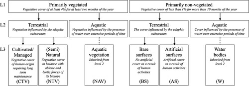
The classification (to LCCS Level 3) was based on the concepts associated with EODESM implemented through the Living Earth platform, as a foundation to enabling wider application to include Level 4. Binary raster inputs were generated using one or more EO products for each decision in the hierarchy. In this way, input products were used for multiple binary decisions, masked by previous levels in the hierarchy. The modified LCCS Level 3 framework used in this study (Figure 1) provides six (6) land cover types, requiring only four (4) binary raster inputs.

2.3. Data

The Landsat data is indexed into DEA as ARD, having already been geometrically corrected, converted to surface reflectance, adjusted for solar illumination and viewing angles, and masked for cloud and cloud shadow (Irish 2000; Li et al. 2020; Zhu and Woodcock 2012; Mueller et al. 2016; Lewis et al. 2017). When stored and accessed through DEA, the Landsat ARD allows individual pixel values for the same location to be accessed and interrogated with consistency through time. Several products derived from Landsat ARD were utilised in the hierarchical framework.

2.4. Classification workflow

2.4.1. Level 1

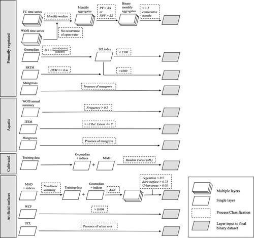
Primarily vegetated areas were identified using time-series analysis of Fractional Cover; a product which utilises a spectral unmixing algorithm to measure green photosynthetic vegetation (FC-PV), non-photosynthetic vegetation (FC-NPV) and bare soil (FC-BS) from each terrain corrected Landsat surface reflectance observation (Gill et al. 2017). Water Observations from Space (WOfS) (described below) was used to mask the occurrence of open water in each observation to avoid erroneous errors associated with Fractional Cover endmembers and water (Guerschman et al. 2009). Similarly, a salt index (SI5; Abbas and Khan 2007) was calculated using annual geometric median pixel composites (Geomedian; Roberts, Mueller, and McIntyre 2017) to mask primarily non-vegetated areas such as mudflats and saltpans that Fractional Cover endmembers did not correctly attribute to BS (Figure 2). Monthly median aggregates were then generated from the masked Fractional Cover observations and used to determine the presence or absence of vegetation. Primarily vegetated areas were defined where the FC-PV or FC-NPV fractions were greater than the FC-BS fraction. These monthly vegetation classifications were then collated and, where the frequency of vegetation presence was two or more consecutive months, the pixel was classified as primarily vegetated. This was considered to meet the FAO LCCS guidelines for primarily vegetated areas. Specific caveats to this method include the inability to confidently define 4% of vegetation cover. However, the criteria were set such that non-vegetated areas needed to demonstrate a majority in the FC-BS endmember (i.e. > 50%).

Figure 2. Input layers and processes adopted to achieve final binary datasets used in hierarchical classification. Layer inputs (grey parallelogram) are binary classifications combined to achieve a final binary dataset. FC; Fractional Cover, PV; photosynthetic vegetation, NPV; non-photosynthetic vegetation, BS; bare soil, WOfS; Water Observations from Space, Geomedian; Landsat geometric median, SI5; salt index 5, SRTM; Shuttle Radar Topographic Mission, ITEM; Intertidal Extent Model, MADs; median absolute deviations, ML; machine learning, ANN; artificial neural network WCF; woody vegetation cover fraction, UCL; urban centre and localities. For Cultivated and Artificial Surfaces indices, see Tables S1 and S2.

2.4.2. Level 2

Aquatic areas were determined using several DEA products applied in combination. Water Observations from Space (WOfS) identifies inland and coastal water bodies through a regression tree classification of Landsat (Mueller et al. 2016). An area was considered aquatic where the presence of water detected was greater than 20% over the annual observations, ensuring infrequent flood events were removed. The Intertidal Extent Model (ITEM) was used to identify non-vegetated intertidal areas such as mud and sand flats (Sagar et al. 2017). This dataset represents the exposed intertidal region of the Australian coastline, based on Landsat observations tagged with reference to corresponding tide heights at the time of image capture. This study applied ITEM to extract aquatic intertidal areas, that is, areas being exposed between 10% and 80% of the tidal range observed by the Landsat archive. National mangrove maps were then used to identify tidally inundated areas not captured by ITEM due to obscuration of water by the mangrove canopy cover (Lymburner et al. 2019). All three data layers were then used in combination to identify aquatic areas, with all those remaining assumed to be terrestrial (Figure 2).

2.4.3. Level 3

Cultivated and managed areas were identified using a supervised machine learning approach. Training data samples were generated for selected Albers tiles using Landsat geometric median images (Geomedians; Roberts, Mueller, and McIntyre 2017) and interpretation confirmed using high resolution imagery from Google Earth^TM for the corresponding years (i.e. training data generated from 2010 and 2015 only). Each tile was segmented in eCognition (to simply group spectrally homogeneous pixels), applying the Normalised Difference Water Index (NDWI) to aggregate and identify water bodies, then manually classifying features to one of five land cover types (cultivated vegetation, n = 5254; natural vegetation, n = 41464; bare areas, n = 995; artificial surface, n = 415; water, n = 2481). Features were selected based on the criteria that they only contain pixels of the required classes and they represent a broad variety of environmental conditions for that class. Each classified training feature was used to extract the median spectral values from two high-dimensional Landsat composite products; annual Geomedians (Roberts, Mueller, and McIntyre 2017), including several spectral indices to enhance differentiation between cultivated areas and other land cover types (see Table S1), and median absolute deviations (MAD; Roberts, Dunn, and Mueller 2018). The MAD dataset identified areas of high and low variability within a calendar year, particularly useful for cultivated areas with distinct sowing, growing and harvesting seasons (Roberts, Dunn, and Mueller 2018).

Training features were selected from a range of locations across Australia to account for variability in climate and cultivated type (e.g. rainfed, irrigated). Features were collated, randomised, and stratified on the five land cover types to provide a balanced training dataset, achieved through scikit-learn ensemble methods such as ‘random state’ and ‘balanced subsample’ weighting (Pedregosa et al. 2011), to develop a classification model. However, testing showed that training on binary data produced more accurate results so the input data was merged to represent just two classes, cultivated areas and counter examples (i.e. natural vegetation, naturally bare surface, artificial surface, water). As an iterative process, several machine learning algorithms were tested with additional training data and features added based on the performance of initial classifications. A Random Forest approach, implemented in scikit-learn (Pedregosa et al. 2011), was selected from this process. Feature selection was conducted using Lasso regression (Tibshirani 1996), this reduced the number of input features to the model (Table S1). The classification model was applied to Landsat Geomedian and MAD datasets where areas classified as cultivated were used as input into LCCS.

Artificial surfaces were differentiated from Bare Surfaces using a deep learning approach, specifically an artificial neural network (ANN). Initially, a continental mask was applied using the MAD dataset to limit false positives due to spectral similarly of salt lakes and other large features in central Australia. Training data was then generated in a semi-automated manner using a non-linear spectral unmixing model based on selected spectral indices for brightness (Tasseled Cap Brightness; Crist 1985), vegetation (Modified Soil Adjusted Vegetation Index; Qi et al. 1994), and water (Modified Normalised Difference Water Index; Xu 2006). The unmixing analysis was used to provide three fractional endmembers based on visual interpretation for Albers tiles covering the Brisbane region. These fractions were labelled based on their broad distinction of vegetation (n = 10000), bare surface (n = 10000), and urban areas (n = 10000). The labelled fractions were then used as model input trained on all Landsat Geomedians bands and several spectral indices (see Table S2, 11 parameters in total). The ANN architecture consisted of four fully connected (dense) layers in sequence (Table S3), implemented with the Keras library (Chollet 2015), using the Tensorflow backend (Abadi et al. 2015). The model was trained for 200 epochs with a batch size of 100, using a Rectified Linear Unit activation function (ReLU) and gradient-based optimisation where the learning rate is adaptive (RMSprop). Thresholds were determined for the three-class output (i.e. three fractions with values that add to 1) through an iterative process (vegetation < 0.5, bare surface > 0.75, urban areas > 0.08) for applying the model to classify Artificial Surfaces. The Woody Cover Fraction (WCF), developed by Liao et al. (2020), was used to further mask naturally bare surfaces (< 0.004) in combination with the Urban Centre and Localities (UCL) map (ABS 2019). The resulting binary mask identifying Artificial Surfaces was used as input to LCCS (Figure 2).

Overall performance of the Cultivated areas model and Artificial surfaces model were evaluated using independent validation data not used in the training of the models. Input variables for each model were evaluated using SHapely Additive exPlanations (SHAP) to identify feature importance (Lundberg and Lee 2017). SHAP values enable fair comparison of input variables to a machine learning model by comparing the model outputs with and without the feature in an iterative process.

2.5. Implementation

The hierarchical classification was executed in Python using the Living Earth software package (Owers et al. 2021), with plugins used to generate custom products. Dataset storage was provided by AWS using S3 and ODC framework of DEA. For implementation, the Australian continent was tiled into 100 km × 100 km Albers tiles (EPSG: 3577) to facilitate distributed compute on AWS. Each tile was classified using the hierarchical approach described in section 2.4. Annual continent-scale land cover maps were produced for the Landsat archive (1988–2020).

2.6. Validation

Validation was completed for the continental-scale land cover maps, using the years (2010 and 2015) for method development and evaluation, in accordance with good practice guidelines (Olofsson et al. 2014; Salk et al. 2018) and FAO accuracy assessment standards (FAO 2016). An overall expected standard error of 0.007 was selected, and the number of points generated was based on proportional area (see Olofsson et al. 2014). Validation points were generated based on the LCCS level 3 output for 2015, stratified to ensure adequate points were selected for each output class based on areal proportion. This stratification was then adjusted to account for the dominant landscape classes across the continent, with 5% more validation points being added to the four under-represented classes and 10% removed from (Semi) Natural Terrestrial Vegetation (NTV) and Bare Surfaces (BS). Final percentages were rounded to the nearest integer prior to generating the standard validation set (Table S4). This resulted in ∼12,000 validation samples (i.e. 6,000 validation points each for 2010 and 2015 annual maps) separated into 60 geographical clusters (∼100 points each cluster) (see Figure S1).

Accuracy assessment was carried out using visual interpretation of annual Geomedians (Roberts, Mueller, and McIntyre 2017) in combination with WOfS (Mueller et al. 2016) and Google Earth^TM / Sentinel-2 imagery for the same epoch where available. Accuracy assessment was manually completed by a small team of remote sensing scientists who observed and followed the same methodology of interpretation, documenting difficult samples, in an effort to enhance consistency and accuracy of the validation set (Wickham et al. 2013; Olofsson et al. 2014; FAO 2016). Each validation team member completed an independent calibration sub-set (∼ 150 points) across the continent to compare visual interpretation consistency between team members (Table S5).

User’s and producer’s accuracy, f-score, quantity and allocation disagreement, as well as overall accuracy, were generated using estimated area proportions, with variance of accuracy measures reported to 95% confidence intervals (Olofsson et al. 2014; FAO 2016). Spatial variation of accuracy was mapped, stratified on major climate groups (Beck et al. 2018), to visualise the performance of the LCCS Level 3 taxonomy. Area proportions were used to estimate the area of each LCCS Level 3 class by generating an error matrix as well as 95% confidence intervals for each class.

3. Results

3.1. Land cover classifications

Annual continent-scale land cover maps were produced for Australia from 1988 to 2020 at 25 m resolution (Figure 3). All maps were generated using the same framework with respective Landsat sensor observations for the calendar year. The DEA Land Cover maps are freely available and accessible on DEA Maps (https://maps.dea.ga.gov.au/ – Select ‘Land and vegetation’ > ‘DEA Land Cover’). The open-source software was produced under an Apache 2.0 license and available online (https://bitbucket.org/au-eoed/livingearth_lccs, https://bitbucket.org/geoscienceaustralia/livingearth_australia).

Figure 3. Annual continent-scale land cover maps for Australia from 1988 to 2020. CTV; cultivated terrestrial vegetation, NTV; natural terrestrial vegetation, NAV; natural aquatic vegetation, AS; artificial surfaces, BS; bare surfaces, W; waterbodies. All maps can be accessed on DEA Maps (https://maps.dea.ga.gov.au/).

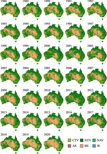
DEA Land Cover demonstrated that the Australian continent was dominated by primarily vegetated areas (> 50%) and interior expanses of primarily bare natural surfaces (> 20%). Artificial surfaces, water bodies and aquatic natural vegetation make up < 5% of the landscape combined, while cultivated and managed areas account for 5–10%. For the selected method development and evaluation years 2010 and 2015, the relative area of land cover classes varied for each year, largely due to considerable differences in rainfall and their influence on vegetation condition (Figures 4 and 5). Waterbodies in 2010 accounted for only 1% of the continental surface, however, this was double the area compared to 2015 (0.45%). Differences in relative area of primarily naturally bare surfaces demonstrate the substantial influence of climate variability on the Australian landscape, with a 10% increase in area for 2015 (2,677,904 km²; 35%) relative to 2010 (1,901,213 km²; 25%).

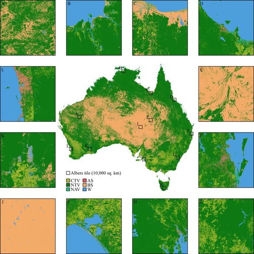
Figure 4. 2010 LCCS Level 3 classification for Australia. Example Albers tiles (100 × 100 km) selected from around the continent. CTV; cultivated terrestrial vegetation, NTV; natural terrestrial vegetation, NAV; natural aquatic vegetation, AS; artificial surfaces, BS; bare surfaces, W; waterbodies. All maps can be accessed on DEA Maps (https://maps.dea.ga.gov.au/).

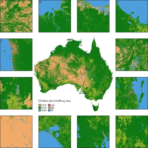
Figure 5. 2015 LCCS Level 3 classification for Australia. Example Albers tiles selected from around the continent. CTV; cultivated terrestrial vegetation, NTV; natural terrestrial vegetation, NAV; natural aquatic vegetation, AS; artificial surfaces, BS; bare surfaces, W; waterbodies. All maps can be accessed on DEA Maps (https://maps.dea.ga.gov.au/).

3.2. Level 3 model accuracy

Total input data to the Cultivated areas Random Forests model was 50609 training samples, with 11737 available for independent validation. The Random Forest model had a reported accuracy of 98% and F1-score of 92%. Feature selection using the Lasso regression removed several Landsat bands and indices from the Geomedian dataset (see Table S1), as well as Bray–Curtis distance median absolute deviations (BCDEV) from the MAD dataset. SHAP analysis demonstrated the greatest variable importance of the near-infrared band (NIR) and Euclidian distance median absolute deviations (EDEV), with several vegetation indices also of moderate importance (Figure 6a). Input variables of lesser importance were those relating to built-up areas (BUI), moisture (NDMI) and bare soil (BSI).

Figure 6. Feature importance of input variables for (a) Cultivated areas machine learning model and (b) Artificial Surfaces deep learning model for DEA Land Cover Level 3 classification. Mean SHAP value indicates feature importance for model output. For Cultivated and Artificial Surfaces indices full names and references, see Tables S1 and S2.

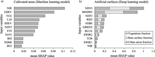
The Artificial surfaces ANN model was trained on total input data size of 54,000 samples, with 6,000 available for independent validation. Final accuracy for the ANN model was 88%, trained for 200 epochs with a batch size of 100, with a reported loss of 0.89. SHAP analysis identified vegetation and water indices, NDVI and MNDWI, as the most prominent input variables impacting model output (Figure 6b). NDVI and MNDWI has substantially higher impact on the model for all output fractions (i.e. vegetation, bare surface, urban areas fractions), having combined mean SHAP values of 1.00 and 0.87 respectively, followed by the tillage index (NDTI) and red band (RED) with only 0.24 and 0.20 respectively. Both the Cultivated areas and Artificial Surfaces models are available on bitbucket (https://bitbucket.org/geoscienceaustralia/livingearth_australia).

3.3. Validation

The overall accuracy of DEA Land Cover annual maps produced using LCCS Level 3 classification was 80%. Validation results discussed here present combined statistics for method evaluation years (2010 and 2015 maps) for the classification approach, however individual statistics for 2010 and 2015 maps are present in the supplementary material. Overall, the summary statistics demonstrate a reasonably robust classification, with high sensitivity (i.e. validation points classified correctly; > 75%, Table 1) and very high specificity (i.e. validation points classified outside of particular category correctly; > 85%, Table 1) across all land cover classes. Allocation and quantity disagreement between validation points and classifications were similar, suggesting that the overall error (i.e. equal to 1 – overall accuracy) was spatially and proportionally distributed (Table 1). However, the exchange component of quantity disagreement (i.e. quantity disagreement = exchange + shift) was substantially greater than the shift, suggesting that the spatial distribution of the overall error was largely due to actual changes in classification. Cultivated and managed areas, as well as naturally bare surfaces, showed substantially higher rates of false discovery (CTV; 45.1%, BS; 41.0%) compared to all other land cover classes (Table 1), reflecting likely confusion in the classification of cultivated and managed areas, and spectral similarity of naturally bare surfaces to other land cover classes.

Table 1. Combined summary statistics (2010 and 2015) for validation points (n = 11737) of the LCCS Level 3 maps.

	Sensitivity (%)	Specificity (%)	False discovery rate (%)
CTV	80.8	94.5	45.1
NTV	77.6	86.3	10.2
NAV	93.5	99.9	1.9
AS	85.1	99.9	3.4
BS	76.6	88.6	41.0
W	97.0	99.7	6.5
Overall Accuracy ± 95 CI		0.80 ± 0.01
Allocation Disagreement		0.11
Shift		0.004
Exchange		0.11
Quantity Disagreement		0.09
AMI		1.03
AMI Adjusted ± 95 CI		1.03 ± 0.03

Note: CTV; cultivated terrestrial vegetation, NTV; natural terrestrial vegetation, NAV; natural aquatic vegetation, AS; artificial surfaces, BS; bare surfaces, W; waterbodies, CI; Confidence Interval, AMI; Average Mutual Information. Individual summary statistics for 2010 and 2015 maps are provided in the supplementary material (2010, Table S6; 2015, Table S7).

The combined error matrix demonstrates patterns of misinterpretation by the classification (Table 2). Naturally bare surfaces and natural terrestrial vegetation were somewhat misclassified with each other, suggesting spectral similarity of endmember fractions in the Fractional Cover product. Similarly, cultivated and managed areas were sometimes misinterpreted as natural terrestrial vegetation but were rarely misclassified as another land cover class. Natural aquatic vegetation, artificial surfaces, and waterbodies presented the least misinterpretation or misclassification, with both user’s and producer’s accuracies > 85%.

Table 2. Combined error matrix (2010 and 2015) for validation points (n = 11737) of the LCCS Level 3 classification.

	CTV	NTV	NAV	AS	BS	W	Total	UA (%) ± 95 CI
CTV	729	559	4	1	35	0	1328	54.89 ± 2.68
NTV	162	5543	6	22	439	2	6174	89.78 ± 0.76
NAV	0	4	575	1	2	4	586	98.12 ± 1.10
AS	0	8	0	430	6	1	445	96.63 ± 1.68
BS	11	1026	2	51	1581	8	2679	59.01 ± 1.86
W	0	4	28	0	2	491	525	93.52 ± 2.11
Total	902	7144	615	505	2065	506	11737
PA (%) ± 95 CI	80.82 ± 2.40	77.59 ± 0.68	93.5 ± 1.85	85.15 ± 2.85	76.56 ± 1.65	97.04 ± 1.46

Note: CTV; cultivated terrestrial vegetation, NTV; natural terrestrial vegetation, NAV; natural aquatic vegetation, AS; artificial surfaces, BS; bare surfaces, W; waterbodies, UA; User’s Accuracy, PA; Producer’s Accuracy. Individual error matrix for 2010 and 2015 maps are provided in the supplementary material (2010, Table S8; 2015, Table S10), and the proportional area error matrix (2010, Table S9; 2015, Table S11).

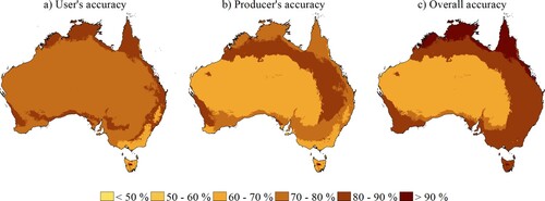
The classification accuracy was spatially variable across the continent, with greater accuracy recorded for tropical (UA = 86%, PA = 76%, OA = 96%) and sub-tropical (UA = 78%, PA = 80%, OA = 88%) climate zones (Figure 7). The reduced accuracies of interior arid zones (UA = 79%, PA = 70%, OA = 68%) likely reflect the misinterpretation and misclassification between natural terrestrial vegetation and naturally bare surfaces that dominate arid landscapes. Reasonably high accuracies were observed in Australia’s agricultural expanses, demonstrating a robust classification of cultivated and managed areas in mixed agricultural landscapes. Similarly, high accuracies in populated coastal regions (i.e. southeast, southwest) demonstrated the capacity of the LCCS Level 3 approach to classify climate regions with complex landscapes.

Figure 7. Combined spatial accuracy map (2010 and 2015) showing mean User’s, Producer’s and Overall accuracy for LCCS Level 3 classification stratified according to Koppen-Gieger climate zones (Beck et al. 2018). Individual spatial accuracy maps for 2010 and 2015 are provided in the supplementary material (2010, Figure S2; 2015, Figure S3).

4. Discussion

This study provides annual continental-scale land cover maps (1988–2020) for Australia and its territories from Landsat sensor data delivered through the ODC platform. Our framework provides a standardised and repeatable approach to land cover mapping utilising an internationally recognised taxonomy in the FAO LCCS Level 3, implemented using the open-source Living Earth system for EO data, with this based on the concepts used in EODESM. Six (6) key land cover classes were generated using this approach, with this requiring only four (4) binary input layers representing vegetated, aquatic, cultivated and artificial landscapes. The DEA instance of the ODC platform was used for developing input environmental descriptors for the Living Earth system, taking full advantage of the Landsat time series to generate annual land cover maps at 25 m spatial resolution. This approach was guided by FAIR principles for software design (Wilkinson et al. 2016) to ensure a nationally operational, open-access mapping product. Map outputs presented here are important for systematic identification of landscape change at scales ranging from continental to sub-national. The LCCS Level 3 classification provides foundational metrics required for reporting on national and international policies and environmental accounting, as well as capacity for more detailed attribution based on LCCS Level 4.

4.1. Annual land cover maps

The overall accuracy of the annual land cover maps generated was 80%, with select assessment year 2015 having marginally greater accuracy (82%) compared to 2010 (78%). This is consistent with other continental-scale maps utilising moderate resolution satellite data (Pflugmacher et al. 2019; Homer et al. 2020; Yang and Huang 2021). The DLCD reports map accuracy using fuzzy logic, where the ‘exact’ and ‘very similar’ matches are 30% and 35% respectively (Lymburner et al. 2011). Although these may appear as low accuracy outputs, the DLCD generated 35 independent classes based on the LCCS Level 4. Therefore, a comparative overall accuracy for DLCD Level 3 can be interpreted as 65%, lower than map accuracies of DEA Land Cover (80%). More recent efforts demonstrate that greater accuracy can be achieved for the Australian continental at 30 m resolution (∼93% overall accuracy, Calderón-Loor, Hadjikakou, and Bryan 2021), though accomplished for 5-year epochs rather than annual time steps, for six user defined classes rather than a standard taxonomic framework. It is important to note that unlike many other land cover products, the accuracy of the land cover products generated in this study are a direct consequence of the four binary input layers, not the final six thematic classes. This approach, therefore, provides a highly flexible and robust platform for generating land cover products that is not grounded on the quality of reference data, or a particular machine learning approach for generating end classes. This is likely at the expense of some map accuracy. However, achieving higher overall accuracy may require compromise on the land cover taxonomy (e.g. use of spectrally similar ‘other areas’ that cannot be identified, see Calderón-Loor, Hadjikakou, and Bryan 2021), reducing the useability of the map product for multiple purposes.

The accuracy obtained for the six land cover classes was similar for 2010 and 2015, with natural aquatic vegetation (99.8% = 2010, 99.6% = 2015), waterbodies (99.8% = 2010, 99.6% = 2015), and artificial surfaces (99.9% = 2010, 99.9% = 2015) recording the highest classification accuracy. Natural aquatic vegetation and waterbodies were primarily derived using existing validated products (e.g. Mangroves = 97.9 - 98.5%, Lymburner et al. 2019; WOfS = 97%, Mueller et al. 2016), contributing to their impressive classification accuracies, whereas artificial surfaces utilised state-of-the-art deep learning techniques that have demonstrated substantial promise in mapping land covers (e.g. Parente et al. 2019; Amani et al. 2020). Naturally bare surfaces proved challenging to classify correctly, with considerable confusion occurring with natural terrestrial vegetated areas. This is reflective of the reduced accuracies for the interior arid regions of Australia, which are dominated by naturally bare and sparsely vegetated landscapes (Walter and Breckle 1986; Donohue, McVicar, and Roderick 2009; McFarlane and Wallace 2019). This confusion has been recognised in similar arid environments when producing continental mapping products (Gong et al. 2019; Venter and Sydenham 2021), as well as limitations with the Fractional Cover product utilised to determine vegetated and non-vegetated areas (Guerschman et al. 2009; Gill et al. 2017; Hill and Guerschman 2020). Moreover, evidence of temporal climatic variability (e.g. year’s with above average rainfall) across the continent have substantial impact on natural terrestrial vegetated area classifications due to greening of sparsely vegetated landscapes (e.g. Figure 3; 2000 and 2011).

Similarly, reduced classification accuracy was recorded for cultivated and managed areas. Evidence of misclassification and confusion is present in tropical areas of the continent, with this attributed in part to the monsoonal seasonal variation of natural vegetation that mimics similar growth patterns observed for cultivated areas (Huete et al. 2006; Poulter and Cramer 2009; Bégué et al. 2018). Notably, the classification was largely correct in areas of cultivation and high land use management (southeast and southwest temperate regions of Australia), suggesting that the machine learning approach utilised in this study has a high classification accuracy in areas of known relevance (i.e. agricultural expanses).

4.2. Land cover classifications using EODESM and Living Earth software

The FAO LCCS is a globally relevant taxonomy with semantics that support and align with end-user requirements (Atyeo and Thackway 2006; Kosmidou et al. 2014; Di Gregorio 2016). The EODESM hierarchical approach, fully implemented in the Living Earth software, facilitates direct comparison between map outputs (Lucas et al. 2019, 2020; Planque et al. 2020; Owers et al. 2021). The four binary input layers used to generate six land cover classes through a range of methods, including a time-series rule-based approach at Level 1, existing aquatic products for Level 2, and a range of machine learning techniques at Level 3, demonstrate the simplicity and flexibility of EODESM in that it enables tailoring and adapting a range of methods for different thematic classes. The hierarchical classification of LCCS Level 3 means that regardless of the environmental descriptors used to form the binary layer inputs, map comparisons will be valid, as the same taxonomic end classes are used. The approach implemented in this study can be applied broadly, to produce spatially and temporally comparable map outputs; a unique feature compared to other continental scale land cover classifications of Australia, providing a straightforward approach for application regardless of geographical context.

In addition, the hierarchical classification approach is adaptive to technological advances in EO sensors and image processing, ensuring longevity of the standardised cartography of land covers. This is a major limitation of other land cover products, and it affects the life cycle of national and continental-scale maps (Wulder et al. 2018; Li et al. 2020; Venter and Sydenham 2021). As higher accuracy environmental descriptor layers become available for implementations such as DEA Land Cover, they are simply substituted or added into the hierarchical framework to generate the next annual land cover product, where the end class taxonomy and hierarchical implementation provide consistent and comparable outputs to previously generated maps. This is currently not possible for many national and continental-scale land cover products underpinned by reference data to train models (e.g. Inglada et al. 2017; Griffiths, Nendel, and Hostert 2019; Malinowski et al. 2020; Zhang et al. 2020; Calderón-Loor, Hadjikakou, and Bryan 2021; Yang and Huang 2021; Brown et al. 2022). Moreover, as a machine learning model becomes superseded in favour of newer models that produce greater accuracy (e.g. spatial and temporal convolutional neural networks in favour of single pixel-based classifications), this will result in maps that are not standardised or comparable, where end classes are generated directly from model classification. This is likely to limit the use of a particular land cover programme for ongoing use and future development.

4.3. Current caveats and future opportunities

While this study has demonstrated the benefits of using the EODESM for generating land cover maps, there are some conceptual limitations which are important to acknowledge. The hierarchical approach of the EODESM means classification accuracy of higher levels (i.e. Level 1 and 2) are inherited by lower levels (i.e. Level 3). For example, if an area in the landscape is naturally bare and incorrectly classified at Level 1 or 2, then correct classification at Level 3 (i.e. differentiation from artificial surfaces) will be irrelevant. This can have additional adverse effects, for instance, if incorrectly classified at Level 1 to primarily vegetated, it may become systematically misinterpreted down the hierarchy and attributed to an incorrect class. If the naturally bare surface is incorrectly classified as natural vegetation at Level 1, then at Level 3 it may have spectral characteristics similar to cultivated and managed areas. The map accuracy statistics may then suggest the cultivated and managed areas machine learning model is an inaccurate classifier. However, this actually represents a misclassification propagated in the hierarchy. This limitation is inherent to hierarchical classifications. However, it demonstrates that implementation of this approach should invest greater resources to ensuring the binary input layer accuracy is greatest at Level 1 and Level 2 before higher accuracies differentiating end classes at Level 3 can be achieved.

The modified FAO LCCS Level 3 framework presented in this paper does not differentiate between natural and artificial waterbodies (such as reservoirs, canals and artificial lakes) nor natural and cultivated aquatic areas (such as rice). This was primarily due to the difficulty of accurate and routine retrieval from EO for these categories based on the FAO LCCS taxonomic definitions (see Di Gregorio 2005; Owers et al. 2021). For example, cultivated aquatic areas in Australia (predominately rice with comparatively high water use efficiency, see Humphreys et al. (2006), Bajwa and Chauhan (2017)) rarely have surface water covering herbaceous vegetation that can be accurately detected from the Landsat sensor data. Instead, land cover characteristics are presented that are spectrally similar to irrigated cultivated and managed areas. Similarly, artificial and natural waterbodies are primarily identified through shape rather than spectral characteristics, with artificial waterbodies having more uniform and rigid extent boundaries. Although many studies have used object-based analysis and machine learning approaches over traditional pixel-based classification, we lack consistent evidence of a robust spatiotemporal techniques that can be applied consistently at a continental scale. Correct and complete identification of these land covers is highly valuable for detecting anthropogenic impacts on landscape change. Future development of these input layers for LCCS level 3 classes would be highly beneficial, and the operational implementation of DEA Land Cover provides the opportunity to develop image processing methods that can be easily integrated into the existing workflow. As the software implementation has been fully designed, interim ancillary products can be easily added within the Living Earth system, such as the Australian Hydrological Geospatial Fabric (Geofabric) to map artificial hydrological features (Atkinson et al. 2008). Further opportunities exist to generate additional environmental descriptors for LCCS Level 4 (additional descriptors for each Level 3 class mapped in this study) that provide detailed land cover descriptions for end users (Owers et al. 2021).

4.4. Application of DEA Land Cover

This study presents a standardised approach to operational implementation of the FAO LCCS Level 3 at national and continental scales. To ensure robust and routinely producible land cover maps, we employ an open-source approach underpinned by the ODC platform, using free and accessible Landsat sensor data (Woodcock et al. 2008) and guided by the FAIR principles of software development. All DEA Land Cover products and metadata are available through DEA Maps (https://maps.dea.ga.gov.au). For DEA Land Cover, two important functions can be implemented in the short to medium term that will enhance ongoing capacity to map and monitor landscape change over the entire Australian continent.

1. DEA Land Cover provides a nationally consistent picture, with the six land cover classes identifying broad land cover categories that are consistent over time and can be compared to detect change. This is highly valuable for retrospective identification of landscape changes over the past 30 years (using the Landsat archive) and into the future (using Landsat and Sentinel sensors), without caveats of jurisdictional boundaries or interoperable land cover taxonomies. Landscape change is a particularly valuable metric derived from multi-temporal land cover maps, and has been demonstrated using the EODESM, where 64 categories of LCCS Level 3 change are identified (Lucas et al. 2019, 2022). This approach could be successfully implemented and extended using the DEA Land Cover products.

2. The LCCS Level 3 output maps provide the foundation for implementing the FAO LCCS Level 4, an attribution-based thematic classification (Di Gregorio 2005, 2016). Delivering a robust Level 3 classification is crucial to providing high confidence in the Level 4 attribution. Level 4 provides more detail to each Level 3 category as available (e.g. canopy cover, water persistence, crop type – see example from Planque et al. 2021) and has been systemically implemented and optimised for EO data (Owers et al. 2021). Existing continental products could be used to derive Level 4 attributes and integrated seamlessly with DEA Land Cover.

DEA Land Cover products have been developed to support national and international reporting that require land cover and land cover change information for routine reporting, such as Sustainable Development Goals (SDGs) and the System of Environmental Economic Accounting (SEEA). EO capacity to support SDGs has been well established (e.g. Paganini et al. 2018; EO4SDGs 2020; Estoque 2020), where maps that produce information for action are required, rather than simply satellite ARD (Metternicht, Mueller, and Lucas 2020; Mohamed-Ghouse et al. 2021). LCCS-based land cover maps can support several SDGs (see Metternicht, Mueller, and Lucas 2020; Owers et al. 2021) and similarly, routine generation of land cover provides consistent and comparable quantification of landscape change for national land and environment accounts. This is particularly useful to address discrepancies across reporting mechanisms, by utilising the same routinely generated national land cover product, and following the principles of good data and information management; ‘collect once, use many times’ (IGGI 2005).

5. Conclusion

DEA Land Cover provides annual continental-scale land cover maps for Australia and its territories using Landsat sensor data from 1988 to 2020. This is generated at a national operational level through Digital Earth Australia using the ODC platform. This study presents a standardised and repeatable approach to land cover mapping utilising an internationally recognised taxonomy in the FAO LCCS, implemented using the open-source Living Earth system that has been optimised for EO data. We developed and evaluated the approach on two calendar years (2010 and 2015) representing the range of climatic conditions experienced on the Australian continent, achieving an overall map accuracy of 80%. The hierarchical structure implemented in FAO LCCS ensures the longevity of the land cover taxonomy, where resources can focus on generating high quality environmental descriptors to be utilised for producing layers that do not alter taxonomic class outputs. Moreover, this study provides key land cover classes (LCCS Level 3) that encourage generation of environmental descriptors for further attribution to landscape descriptions (LCCS Level 4). Map outputs presented here are important for systematic identification of landscape change at scales ranging from the continental to sub-national and can therefore provide foundational measurements required for reporting on national and international policies and environmental accounts.

Acknowledgements

The authors would like to thank the Digital Earth Australia team for their assistance in several aspects of producing DEA Land Cover; from development and feedback of product iterations, to DevOps challenges, ensuring any roadblocks were quickly overcome. We really appreciate the help of Ben Lewis, Cate Kooymans, Eloise Birchall and Erin Telfer who were part of the validation team. Thank you also to Stephen Sagar and Simon Oliver who reviewed this manuscript. This paper was published with the permission of the CEO, Geoscience Australia.

Data availability

The data and code that support the findings of this study are openly available. The open-source software was produced under an Apache 2.0 license and available online (https://bitbucket.org/au-eoed/livingearth_lccs, https://bitbucket.org/geoscienceaustralia/livingearth_australia). All maps can be accessed on DEA Maps (https://maps.dea.ga.gov.au/) and are provided under CC BY Attribution 4.0 International License. All dataset information is available online (https://cmi.ga.gov.au/data-products/dea/607/dea-land-cover-landsat).

Disclosure statement

No potential conflict of interest was reported by the author(s).

Additional information

Funding

This research has been conducted with the support of Geoscience Australia, through the DEA Land Cover project, and the European Regional Development Fund (ERDF) Sêr Cymru II programme award [grant number 80761-AU-108; Living Wales].

References

- Abadi, M., A. Agarwal, P. Barham, E. Brevdo, Z. Chen, C. Citro, G. S. Corrado, et al. 2015. Tensorflow: Large-Scale Machine Learning on Heterogeneous Systems. https://tensorflow.org
- Abbas, A., and S. Khan. 2007. “Using Remote Sensing Techniques for Appraisal of Irrigated Soil Salinity.” Proceedings of the International Congress on Modelling and Simulation, Christchurch, New Zealand, December 10–13.
- ABS. 2012. Year Book Australia: Geography and Climate. Australia Bureau of Statistics, Canberra, Australia. Accessed September 19, 2022. https://www.abs.gov.au/ausstats/[email protected]/Lookup/by%20Subject/1301.0~2012~Main%20Features~Geography%20of%20Australia~12.
- ABS. 2019. Australian Statistical Geography Standard (ASGS) Volume 4 – Significant Urban Areas, Urban Centres and Localities, Section of State (cat no. 1270.0.55.004). Australia Bureau of Statistics, Canberra, Australia. Accessed September 19, 2022. https://www.abs.gov.au/AUSSTATS/[email protected]/Lookup/1270.0.55.004Main+Features1July%202016?OpenDocument.
- Amani, M., M. Kakooei, A. Moghimi, A. Ghorbanian, B. Ranjgar, S. Mahdavi, A. Davidson, et al. 2020. “Application of Google Earth Engine Cloud Computing Platform, Sentinel Imagery, and Neural Networks for Crop Mapping in Canada.” Remote Sensing 12: 3561. doi:10.3390/rs12213561.
- Asbridge, E., R. Bartolo, C. Finlayson, R. Lucas, K. Rogers, and C. Woodroffe. 2019. “Assessing the Distribution and Drivers of Mangrove Dieback in Kakadu National Park, Northern Australia.” Estuarine, Coastal and Shelf Science 228: 106353. doi:10.1016/j.ecss.2019.106353.
- Atkinson, R., R. Power, D. Lemon, R. O’Hagan, D. Dovey, and D. Kinny. 2008. The Australian Hydrological Geospatial Fabric - Development Methodology and Conceptual Architecture. CSIRO: Water for a Healthy Country National Research Flagship, Canberra, Australia.
- Atyeo, C., and R. Thackway. 2006. Classifying Australian Land Cover. Canberra, Australia: Bureau of Rural Sciences.
- Bajwa, A. A., and B. S. Chauhan. 2017. “Rice Production in Australia.” In Rice Production Worldwide, edited by B. S. Chauhan, K. Jabran, and G. Mahajan, 169–184. Basel, Switzerland: Springer Nature.
- Beck, H. E., N. E. Zimmermann, T. R. McVicar, N. Vergopolan, A. Berg, and E. F. Wood. 2018. “Present and Future Köppen-Geiger Climate Classification Maps at 1-km Resolution.” Scientific Data 5: 1–12. doi:10.1038/sdata.2018.214.
- Bégué, A., D. Arvor, B. Bellon, J. Betbeder, D. de Abelleyra, R. P. D. Ferraz, V. Lebourgeois, C. Lelong, M. Simões, and S. R. Verón. 2018. “Remote Sensing and Cropping Practices: A Review.” Remote Sensing 10 (1): 1–32. doi:10.3390/rs10010099.
- Bishop-Taylor, R., S. Sagar, L. Lymburner, and R. J. Beaman. 2019. “Between the Tides: Modelling the Elevation of Australia’s Exposed Intertidal Zone at Continental Scale.” Estuarine, Coastal and Shelf Science 223: 115–128. doi:10.1016/j.ecss.2019.03.006.
- Boer, M. M., V. R. de Dios, and R. A. Bradstock. 2020. “Unprecedented Burn Area of Australian Mega Forest Fires.” Nature Climate Change 10: 171–172. doi:10.1038/s41558-020-0716-1.
- BOM. 2011. “Record-breaking La Niña Events.” Australia Government Bureau of Meteorology, Melbourne, Australia. Accessed September 19, 2022. http://www.bom.gov.au/climate/enso/history/La-Nina-2010-12.pdf.
- BOM. 2016. “Annual Climate Report 2015. “Australia Government Bureau of Meteorology, Melbourne, Australia. Accessed September 19, 2022. http://www.bom.gov.au/climate/annual_sum/2015/Annual-Climate-Report-2015-HR.pdf.
- Brown, C. F., S. P. Brumby, B. Guzder-Williams, T. Birch, S. Brooks Hyde, J. Mazzariello, W. Czerwinski, et al. 2022. “Dynamic World, Near Real-Time Global 10 m Land use Land Cover Mapping.” Scientifc Data 9: 251. doi:10.1038/s41597-022-01307-4.
- Calderón-Loor, M., M. Hadjikakou, and B. A. Bryan. 2021. “High-resolution Wall-to-Wall Land-Cover Mapping and Land Change Assessment for Australia from 1985 to 2015.” Remote Sensing of Environment 252), doi:10.1016/j.rse.2020.112148.
- Chollet, F. 2015. Keras. https://keras.io
- Clark, G. F., and E. L. Johnston. 2017. Australia State of the Environment 2016: Coasts, Independent Report to the Australian Government Minister for Environment and Energy, Australian Government Department of the Environment and Energy, Canberra.
- Crist, E. 1985. “A TM Tasseled Cap Equivalent Transformation for Reflectance Factor Data.” Remote Sensing of Environment 17 (3): 301–206.
- Díaz, S., J. Settele, B. Eduardo, H. T. Ngo, M. Guèze, J. Agard, A. Arneth, et al. 2019. “The Global Assessment Report on Report on Biodiversity and Ecosystem Services. Summary for Policymakers.” IPBES: Bonn, Germany.
- Dhu, T., B. Dunn, B. Lewis, L. Lymburner, N. Mueller, E. Telfer, A. Lewis, A. McIntyre, S. Minchin, and C. Phillips. 2017. “Digital Earth Australia – Unlocking New Value from Earth Observation Data.” Big Earth Data 1: 64–74. doi:10.1080/20964471.2017.1402490.
- Di Gregorio, A. 2005. Land Cover Classification System: Classification Concepts and User Manual, Software Version 2. Rome: Food and Agriculture Organization of the United Nations.
- Di Gregorio, A. 2016. Land Cover Classification System User Manual, Software version 3. Food and Agriculture Organization of the United Nations, Rome. Accessed September 19, 2022. http://www.fao.org/3/i5428e/i5428e.pdf.
- Di Gregorio, A., and L. J. M. Jansen. 2000. Land Cover Classification System – Classification Concepts and User Manual. Food and Agriculture Organization of the United Nations, Rome. Accessed September 19, 2022. http://www.fao.org/3/x0596e/x0596e00.htm.
- Donohue, R. J., T. R. McVicar, and M. L. Roderick. 2009. “Climate-related Trends in Australian Vegetation Cover as Inferred from Satellite Observations 1981–2006.” Global Change Biology 15 (4): 1025–1039. doi:10.1111/j.1365-2486.2008.01746.x.
- Duke, N. C., J. M. Kovacs, A. D. Griffiths, L. Preece, D. J. E. Hill, P. van Oosterzee, J. Mackenzie, H. S. Morning, and D. Burrows. 2017. “Large-scale Dieback of Mangroves in Australia’s Gulf of Carpentaria: A Severe Ecosystem Response, Coincidental with an Unusually Extreme Weather Event.” Marine and Freshwater Research 68: 1816–1829. doi:10.1071/MF16322.
- EO4SDG. 2020. “Earth Observations in Services of the 2030 Agenda for Sustainable Development.” Accessed September 19, 2022. https://earthobservations.org/documents/gwp20_22/eo_for_sustainable_development_goals_ip.pdf.
- Estoque, R. C. 2020. “A Review of the Sustainability Concept and the State of SDG Monitoring Using Remote Sensing.” Remote Sensing 12 (11): 1770. doi:10.3390/rs12111770.
- FAO. 2016. “Map Accuracy Assessment and Area Estimation: A Practical Guide.” National Forest Monitoring Assessment Working Paper,E (46), 69. United Nations Food and Agricultural Organisation. Accessed September 19, 2022. http://www.fao.org/3/a-i5601e.pdf.
- Franklin, S. E., and M. A. Wulder. 2002. “Remote Sensing Methods in Medium Spatial Resolution Satellite Data Land Cover Classification of Large Areas.” Progress in Physical Geography 26 (2): 173–205. doi:10.1191/0309133302pp332ra.
- Geoscience Australia. 1994. “Geoscience Australia Deserts Database.” Geoscience Australia, Canberra, Australia. Accessed September 19, 2022. https://www.ga.gov.au/scientific-topics/national-location-information/landforms/deserts.
- Ghorbanian, A., M. Kakooei, M. Amani, S. Mahdavi, A. Mohammadzadeh, and M. Hasanlou. 2020. “Improved Land Cover Map of Iran Using Sentinel Imagery within Google Earth Engine and a Novel Automatic Workflow for Land Cover Classification Using Migrated Training Samples.” ISPRS Journal of Photogrammetry and Remote Sensing 167: 276–288. doi:10.1016/j.isprsjprs.2020.07.013.
- Gill, T., K. Johansen, S. Phinn, R. Trevithick, P. Scarth, and J. A. Armston. 2017. “A Method for Mapping Australian Woody Vegetation Cover by Linking Continental-Scale Field Data and Long-Term Landsat Time Series.” International Journal of Remote Sensing 38: 679–705. doi:10.1080/01431161.2016.1266112.
- Gills, B., and J. Morgan. 2020. “Global Climate Emergency: After COP24, Climate Science, Urgency, and the Threat to Humanity.” Globalizations 17 (6): 885–902. doi:10.1080/14747731.2019.1669915.
- Gómez, C., J. C. White, and M. A. Wulder. 2016. “Optical Remotely Sensed Time Series Data for Land Cover Classification: A Review.” ISPRS Journal of Photogrammetry and Remote Sensing 116: 55–72. doi:10.1016/j.isprsjprs.2016.03.008.
- Gong, P., H. Liu, M. Zhang, C. Li, J. Wang, H. Huang, N. Clinton, et al. 2019. “Stable Classification with Limited Sample: Transferring a 30-m Resolution Sample set Collected in 2015 to Mapping 10-m Resolution Global Land Cover in 2017.” Science Bulletin 64 (6): 370–373. doi:10.1016/j.scib.2019.03.002.
- Grekousis, G., G. Mountrakis, and M. Kavouras. 2015. “An Overview of 21 Global and 43 Regional Land-Cover Mapping Products.” International Journal of Remote Sensing 36 (21): 5309–5335. doi:10.1080/01431161.2015.1093195.
- Griffiths, P., C. Nendel, and P. Hostert. 2019. “Intra-annual Reflectance Composites from Sentinel-2 and Landsat for National-Scale Crop and Land Cover Mapping.” Remote Sensing of Environment 220: 135–151. doi:10.1016/j.rse.2018.10.031.
- Guerschman, J. P., M. J. Hill, L. J. Renzullo, D. J. Barrett, A. S. Marks, and E. J. Botha. 2009. “Estimating Fractional Cover of Photosynthetic Vegetation, non- Photosynthetic Vegetation and Bare Soil in the Australian Tropical Savanna Region Upscaling the EO- 1 Hyperion and MODIS Sensors.” Remote Sensing of Environment 113 (5): 928–945. doi:10.1016/j.rse.2009.01.006.
- Harwood, T. D., R. J. Donohue, K. J. Williams, S. Ferrier, T. R. McVicar, G. Newell, and M. White. 2016. “Habitat Condition Assessment System: A new way to Assess the Condition of Natural Habitats for Terrestrial Biodiversity Across Whole Regions Using Remote Sensing Data.” Methods in Ecology and Evolution 7 (9): 1050–1059. doi:10.1111/2041-210X.12579.
- Herold, M., L. See, N. E. Tsendbazar, and S. Fritz. 2016. “Towards an Integrated Global Land Cover Monitoring and Mapping System.” Remote Sensing 8 (12): 1–11. doi:10.3390/rs8121036.
- Hill, M. J., and J. P. Guerschman. 2020. “The MODIS Global Vegetation Fractional Cover Product 2001–2018: Characteristics of Vegetation Fractional Cover in Grasslands and Savanna Woodlands.” Remote Sensing 12 (3): 406. doi:10.3390/rs12030406.
- Homer, C., J. Dewitz, S. Jin, G. Xian, C. Costello, P. Danielson, L. Gass, et al. 2020. “Conterminous United States Land Cover Change Patterns 2001–2016 from the 2016 National Land Cover Database.” ISPRS Journal of Photogrammetry and Remote Sensing 162: 184–199. doi:10.1016/j.isprsjprs.2020.02.019.
- Huete, A. R., K. Didan, Y. E. Shimabukuro, P. Ratana, S. R. Saleska, L. R. Hutyra, W. Yang, R. R. Nemani, and R. Myneni. 2006. “Amazon Rainforests Green-up with Sunlight in dry Season.” Geophysical Research Letters 33 (6): 2–5. doi:10.1029/2005GL025583.
- Humphreys, E., L. G. Lewin, S. Khan, H. G. Beecher, J. M. Lacy, J. A. Thompson, G. D. Batten, et al. 2006. “Integration of Approaches to Increasing Water use Efficiency in Rice-Based Systems in Southeast Australia.” Field Crops Research 97 (1 SPEC. ISS.): 19–33. doi:10.1016/j.fcr.2005.08.020.
- IGGI. 2005. “The Principles of Good Data Management.” Intragovernmental Group on Geographic Information. Data Management, 1–35.
- Inglada, J., A. Vincent, M. Arias, B. Tardy, D. Morin, and I. Rodes. 2017. “Operational High Resolution Land Cover Map Production at the Country Scale Using Satellite Image Time Series.” Remote Sensing 9: 95. doi:10.3390/rs9010095.
- Irish, R. R. 2000. “Landsat 7 Automatic Cloud Cover Assessment.” In AeroSense 2000, International Society for Optics and Photonics, 348–355. doi:10.1117/12.410358
- Kavvada, A., G. Metternicht, F. Kerblat, N. Mudau, M. Haldorson, S. Laldaparsad, L. Friedl, A. Held, and E. Chuvieco. 2020. “Towards Delivering on the Sustainable Development Goals Using Earth Observations.” Remote Sensing of Environment 247: 111930. doi:10.1016/j.rse.2020.111930.
- Kosmidou, V., Z. Petrou, R. G. H. Bunce, C. A. Mücher, R. H. G. Jongman, M. M. B. Bogers, R. M. Lucas, et al. 2014. “Harmonization of the Land Cover Classification System (LCCS) with the General Habitat Categories (GHC) Classification System.” Ecological Indicators 36: 290–300. doi:10.1016/j.ecolind.2013.07.025.
- Krause, C. E., V. Newey, M. J. Alger, and L. Lymburner. 2021. “Mapping and Monitoring the Multi-Decadal Dynamics of Australia’s Open Waterbodies Using Landsat.” Remote Sensing 13: 1437. doi:10.3390/rs13081437.
- Lamchin, M., S. W. Wang, C. H. Lim, A. Ochir, U. Pavel, B. M. Gebru, Y. Choi, S. W. Jeon, and W. K. Lee. 2020. “Understanding Global Spatio-Temporal Trends and the Relationship Between Vegetation Greenness and Climate Factors by Land Cover During 1982–2014.” Global Ecology and Conservation 24: e01299. doi:10.1016/j.gecco.2020.e01299.
- Lewis, A., S. Oliver, L. Lymburner, B. Evans, L. Wyborn, N. Mueller, G. Raevksi, et al. 2017. “The Australian Geoscience Data Cube – Foundations and Lessons Learned.” Remote Sensing of Environment 202: 276–292. doi:10.1016/j.rse.2017.03.015.
- Li, Q., C. Qiu, L. Ma, M. Schmitt, and X. X. Zhu. 2020. “Mapping the Land Cover of Africa at 10 m Resolution from Multi-Source Remote Sensing Data with Google Earth Engine.” Remote Sensing 12: 602. doi:10.3390/rs12040602.
- Liao, Z., A. I. J. M. Van Dijk, B. He, P. R. Larraondo, and P. F. Scarth. 2020. “Woody Vegetation Cover, Height and Biomass at 25-m Resolution Across Australia Derived from Multiple Site, Airborne and Satellite Observations.” International Journal of Applied Earth Observation and Geoinformation 93: 102209. doi:10.1016/j.jag.2020.102209.
- Lucas, R. M., S. German, G. Metternicht, R. K. Schmidt, C. J. Owers, S. M. Prober, A. Richards, et al. 2022. “A Globally Relevant Change Taxonomy and Evidence-Based Change Framework for Land Monitoring.” Global Change Biology, 1–25. doi:10.1111/gcb.16346.
- Lucas, R., and A. Mitchell. 2017. “Integrated Land Cover and Change Classifications.” In The Roles of Remote Sensing in Nature Conservation: A Practical Guide and Case Studies, edited by R. Díaz-Delgado, R. Lucas, and C. Hurford, 295–308. Charm, Switzerland: Springer International Publishing.
- Lucas, R., N. Mueller, A. Siggins, C. J. Owers, D. Clewley, P. Bunting, C. Kooymans, et al. 2019. “Land Cover Mapping Using Digital Earth Australia.” Data 4 (4): 143. doi:10.3390/data4040143.
- Lucas, R., V. Otero, R. V. D. Kerchove, D. Lagomasino, B. Satyanarayana, T. Fatoyinbo, and F. Dahdouh-Guebas. 2020. “Monitoring Matang’s Mangroves in Peninsular Malaysia Through Earth Observations: A Globally Relevant Approach.” Land Degradation & Development 32 (1): 354–373. doi:10.1002/ldr.3652.
- Lundberg, S. M., and S. I. Lee. 2017. “A Unified Approach to Interpreting Model Predictions.” Proceedings of the 31st International Conference on Advances in Neural Information Processing Systems, 4765–4774.
- Lymburner, L., P. Bunting, R. Lucas, P. Scarth, I. Alam, C. Phillips, C. Ticehurst, and A. Held. 2019. “Mapping the Multi-Decadal Mangrove Dynamics of the Australian Coastline.” Remote Sensing of Environment 238: 111185. doi:10.1016/j.rse.2019.05.004.
- Lymburner, L., P. Tan, N. Mueller, R. Thackway, and M. Thankappan. 2011. “The National Dynamic Land Cover Dataset - Technical Report.” Record 2011/031. Geoscience Australia, Canberra, Australia. Accessed September 19, 2022. http://www.ga.gov.au/corporate_data/71069/Rec2011_031.pdf.
- Malinowski, R., S. Lewiński, M. Rybicki, E. Gromny, M. Jenerowicz, M. Krupiński, A. Nowakowski, et al. 2020. “Automated Production of a Land Cover/Use Map of Europe Based on Sentinel-2 Imagery.” Remote Sensing 12: 3523. doi:10.3390/rs12213523.
- McFarlane, D. J., and J. F. Wallace. 2019. “Measuring Native Vegetation Extent and Condition Using Remote Sensing Technologies – a Review and Identification of Opportunities.” The Western Australian Biodiversity Science Institute, Perth, Western Australia.
- Metternicht, G., N. Mueller, and R. Lucas. 2020. “Digital Earth for Sustainable Development Goals.” In Manual of Digital Earth, edited by G. Huadong, M. F. Goodchild, and A. Annoni. Singapore: Springer. doi:10.1007/978-981-32-9915-3_13
- Mohamed-Ghouse, Z. S., C. Desha, A. Rajabifard, M. Blicavs, and G. Martin. 2021. “Evaluating the Role of Partnerships in Increasing the use of big Earth Data to Support the Sustainable Development Goals: An Australian Perspective.” Big Earth Data 5 (4): 527–556. doi:10.1080/20964471.2021.1981801.
- Mueller, N., A. Lewis, D. Roberts, S. Ring, R. Melrose, J. Sixsmith, L. Lymburner, et al. 2016. “Water Observations from Space: Mapping Surface Water from 25 Years of Landsat Imagery Across Australia.” Remote Sensing of Environment 174: 341–352. doi:10.1016/j.rse.2015.11.003.
- Olofsson, P., G. M. Foody, M. Herold, S. V. Stehman, C. E. Woodcock, and M. A. Wulder. 2014. “Good Practices for Estimating Area and Assessing Accuracy of Land Change.” Remote Sensing of Environment 148: 42–57. doi:10.1016/j.rse.2014.02.015.
- Owers, C. J., R. M. Lucas, D. Clewley, C. Planque, S. Punalekar, B. Tissott, S. Chua, P. Bunting, N. Mueller, and G. Metternicht. 2021. “Living Earth: Implementing National Standardized Land Cover Classification Systems for Earth Observation in Support of Sustainable Development.” Big Earth Data 5 (3): 368–390. doi:10.1080/20964471.2021.1948179.
- Paganini, M., I. Petiteville, S. Ward, G. Dyke, M. Steventon, J. Harry, and F. Kerblat. 2018. “Satellite Earth Observations in Support of the Sustainable Development Goals.” Accessed September 19, 2022. http://eohandbook.com/sdg/files/CEOS_EOHB_2018_SDG.pdf.
- Parente, L., E. Taquary, A. P. Silva, C. Souza, and L. Ferreira. 2019. “Next Generation Mapping: Combining Deep Learning, Cloud Computing, and big Remote Sensing Data.” Remote Sensing 11: 2881. doi:10.3390/rs11232881.
- Pedregosa, F., G. Varoquaux, A. Gramfort, V. Michel, B. Thirion, O. Grisel, M. Blondel, et al. 2011. “Scikit-learn: Machine Learning in Python.” Journal of Machine Learning Research 12: 2825–2830.
- Peel, M. C., B. L. Finlayson, and T. A. McMahon. 2007. “Updated World map of the Koppen-Geiger Climate Classification. Hydrology and Earth System Sciences Discussions.” European Geosciences Union 4 (2): 439–473. doi:10.5194/hess-11-1633-2007.
- Pflugmacher, D., A. Rabe, M. Peters, and P. Hostert. 2019. “Mapping pan-European Land Cover Using Landsat Spectral-Temporal Metrics and the European LUCAS Survey.” Remote Sensing of Environment 221: 583–595. doi:10.1016/j.rse.2018.12.001.
- Phiri, D., and J. Morgenroth. 2017. “Developments in Landsat Land Cover Classification Methods: A Review.” Remote Sensing 9 (9), doi:10.3390/rs9090967.
- Planque, C., R. Lucas, S. Punalekar, S. Chognard, C. Hurford, C. J. Owers, C. Horton, et al. 2021. “National Crop Mapping Using Sentinel-1 Time Series: A Knowledge-Based Descriptive Algorithm.” Remote Sensing 13: 846. doi:10.3390/rs13050846.
- Planque, C., S. Punalekar, R. Lucas, S. Chognard, C. J. Owers, D. Clewley, P. Bunting, H. Sykes, and C. Horton. 2020. “Living Wales: Automatic and Routine Environmental Monitoring Using Multisource Earth observation Data.” SPIE 11534, Earth Resources and Environmental Remote Sensing/GIS Applications XI, 115340C. doi:10.1117/12.2573763
- Poulter, B., and W. Cramer. 2009. “Satellite Remote Sensing of Tropical Forest Canopies and Their Seasonal Dynamics.” International Journal of Remote Sensing 30 (24): 6575–6590. doi:10.1080/01431160903242005.
- Punalekar, S. M., C. Planque, R. M. Lucas, D. Evans, V. Correia, C. J. Owers, P. Poslajko, P. Bunting, and S. Chognard. 2021. “National Scale Mapping of Larch Plantations for Wales Using the Sentinel-2 Data Archive.” Forest Ecology and Management 501: 119679. doi:10.1016/j.foreco.2021.119679.
- Punalekar, S. M., C. Planque, P. Poslajko, R. Lucas, S. Chognard, C. J. Owers, P. Bunting, D. Clewley, and C. Horton. 2020. “Mapping Dominant Genus/Species Types in Natural and Seminatural Landscapes Across Wales Through Application of Sentinel-2 Time-Series Data.” SPIE 11528. Remote Sensing for Agriculture, Ecosystems, and Hydrology, XXII, 1152805. doi:10.1117/12.2574005
- Qi, J., A. Chehbouni, A. R. Huete, Y. H. Kerr, and S. Sorooshian. 1994. “A Modified Soil Adjusted Vegetation Index.” Remote Sensing of Environment 48 (2): 119–126. doi:10.1016/0034-4257(94)90134-1.
- Roberts, D., B. Dunn, and N. Mueller. 2018. “Open Data Cube Products Using High-Dimensional Statistics of Time Series.” IGARSS IEEE International Geoscience and Remote Sensing Symposium, Valencia, Spain, 8647–8650. doi:10.1109/igarss.2018.8518312
- Roberts, D., N. Mueller, and A. McIntyre. 2017. “High-Dimensional Pixel Composites from Earth Observation Time Series.” IEEE Transactions in Geoscience and Remote Sensing 99: 1–11. doi:10.1109/TGRS.2017.2723896.
- Roberts, D., J. Wilford, and O. Ghattas. 2019. “Exposed Soil and Mineral map of the Australian Continent Revealing the Land at its Barest.” Nature Communications 10: 5297. doi:10.1038/s41467-019-13276-1.
- Sagar, S., D. Roberts, B. Bala, and L. Lymburner. 2017. “Extracting the Intertidal Extent and Topography of the Australian Coastline from a 28 Year Time Series of Landsat Observations.” Remote Sensing of Environment 195: 153–169. doi:10.1016/j.rse.2017.04.009.
- Salk, C., S. Fritz, L. See, C. Dresel, and I. McCallum. 2018. “An Exploration of Some Pitfalls of Thematic map Assessment Using the new map Tools Resource.” Remote Sensing 10 (3): 1–14. doi:10.3390/rs10030376.
- Skidmore, A. K., N. C. Coops, E. Neinavaz, A. Ali, M. E. Schaepman, M. Paganini, W. D. Kissling, et al. 2021. “Priority List of Biodiversity Metrics to Observe from Space.” Nature Ecology and Evolution 5 (7): 896–906. doi:10.1038/s41559-021-01451-x.
- Tibshirani, R. 1996. “Regression Shrinkage and Selection via the Lasso.” Journal of the Royal Statistical Society. Series B (Methodological) 58 (1): 267–288. doi:10.1111/j.2517-6161.1996.tb02080.x.
- Tollefson, J. 2019. “Humans are Driving one Million Species to Extinction.” Nature 569: 171.
- Venter, Z. S., and M. A. K. Sydenham. 2021. “Continental-scale Land Cover Mapping at 10 m Resolution Over Europe (Elc10).” Remote Sensing 13 (12): 1–23. doi:10.3390/rs13122301.
- Walter, H., and S. W. Breckle. 1986. “The Arid Regions of Australia.” In Ecological Systems of the Geobiosphere. Berlin, Heidelberg: Springer. doi:10.1007/978-3-662-06812-0_29
- White, M., P. Griffioen, and G. Newell. 2020. “Multi-temporal Native Vegetation Extent for Victoria. Arthur Rylah Institute for Environmental Research Technical Report No 311.” Department of Environment, Land, Water and Planning. Accessed September 19, 2022. https://www.environment.vic.gov.au/__data/assets/pdf_file/0042/479877/Victorian_Land_Cover_Time_Series_Data_1985-2019_DELWP_ARI_TechReport.pdf.
- Wickham, J. D., S. V. Stehman, L. Gass, J. Dewitz, J. A. Fry, and T. J. Wade. 2013. “Accuracy Assessment of NLCD 2006 Land Cover and Impervious Surface.” Remote Sensing of Environment 130: 294–304. doi:10.1016/j.rse.2012.12.001.
- Wilkinson, M. D., M. Dumontier, Ij Aalbersberg, J. Appleton, G. Axton, M. Baak, A. Blomberg, et al. 2016. “Comment: The FAIR Guiding Principles for Scientific Data Management and Stewardship.” Scientific Data 3: 160018. doi:10.1038/sdata.2016.18.
- Woodcock, C. E., A. A. Allen, M. Anderson, A. S. Belward, R. Bindschadler, W. B. Cohen, F. Gao, et al. 2008. “Free Access to Landsat Imagery.” Science 320: 1011. doi:10.1126/science.320.5879.1011a.
- Wulder, M. A., N. C. Coops, D. P. Roy, J. C. White, and T. Hermosilla. 2018. “Land Cover 2.0.” International Journal of Remote Sensing 39 (12): 4254–4284. doi:10.1080/01431161.2018.1452075.
- Xie, X., B. He, L. Guo, C. Miao, and Y. Zhang. 2019. “Detecting Hotspots of Interactions Between Vegetation Greenness and Terrestrial Water Storage Using Satellite Observations.” Remote Sensing of Environment 231: 111259. doi:10.1016/j.rse.2019.111259.
- Xu, H. 2006. “Modification of Normalised Difference Water Index (NDWI) to Enhance Open Water Features in Remotely Sensed Imagery.” International Journal of Remote Sensing 27 (14): 3025–3033. doi:10.1080/01431160600589179.
- Yang, X., and X. Huang. 2021. “The 30 m Annual Land Cover Dataset and its Dynamics in China from 1990 to 2019.” Earth System Science Data 13: 3907–3925. doi:10.5194/essd-13-3907-2021.
- Yang, H., S. Li, J. Chen, X. Zhang, and S. Xu. 2017. “The Standardization and Harmonization of Land Cover Classification Systems Towards Harmonized Datasets: A Review.” ISPRS International Journal of Geo-Information 6 (5): 154. doi:10.3390/ijgi6050154.
- Zhang, M., H. Huang, Z. Li, K. O. Hackman, C. Liu, R. L. Andriamiarisoa, T. Ny Aina Nomenjanahary Raherivelo, Y. Li, and P. Gong. 2020. “Automatic High-Resolution Land Cover Production in Madagascar Using Sentinel-2 Time Series, Tile-Based Image Classification and Google Earth Engine.” Remote Sensing 12: 3663. doi:10.3390/rs12213663.
- Zhu, Z., and C. E. Woodcock. 2012. “Object-based Cloud and Cloud Shadow Detection in Landsat Imagery.” Remote Sensing of Environment 118: 83–94. doi:10.1016/j.rse.2011.10.028.