A fine-grained evaluation of social vulnerability to COVID-19, healthcare access and built environmental disparities in Tokyo, Japan

ABSTRACT

Measuring vulnerability to COVID-19 and healthcare accessibility at the fine-grained level serves as the foundation for spatially explicit health planning and policy making in response to future public health crises. However, the evaluation of vulnerability and healthcare accessibility is insufficient in Japan – a nation with high population density and super-aging challenges. Drawing on the 2022 census data, transport network, medical and digital cadastral data, land use maps, and points of interest data, our study extends the concept of vulnerability in the context of COVID-19 and constructs the first fine-grained measure of vulnerability and healthcare accessibility in Tokyo Metropolis, Japan – the most populated metropolitan region in the world. We delineate the vulnerable neighbourhoods with low healthcare access and further evaluate the disparity in healthcare access and built environment of areas at different levels of vulnerability. Our outcome datasets and findings provide nuanced and timely evidence to government and health authorities to have a holistic and latest understanding of social vulnerability to COVID-19 and healthcare access at a fine-grained level. Our analytical framework can be employed in different geographic contexts, guiding through place-based health planning and policy making in the post-COVID era and beyond.

KEYWORDS:

• COVID-19
• vulnerability
• healthcare access
• built environment
• network analysis
• Tokyo metropolis

1. Introduction

The ongoing COVID-19 pandemic, which is likely to be long-lasting in the following years, threatens many countries’ national public health systems and has disproportional impacts on people’s daily lives (Sykes et al. 2021; Sha et al. 2021; Hu et al. 2021). Medical resources and services were primarily allocated to COVID-19 treatments which supplanted resources for non-COVID medical care. The redistribution of medical resources and services exacerbated the disparity in healthcare access that has existed in pre-COVID-19 societies (Krouse 2020). On the other hand, the impacts of COVID-19 on people vary across social groups with different demographic and socioeconomic backgrounds (Hawkins, Charles, and Mehaffey 2020). It has been widely witnessed that children and the elderly, people with a low level of socioeconomic status, and certain minorities (e.g. the Hispanic population in the U.S.) are more vulnerable to COVID-19 compared to the general population (Chen et al. 2021; Daoust 2020; Huang et al. 2021; Macias Gil et al. 2020; Zhang et al. 2021). Measuring vulnerability, more importantly, identifying vulnerable communities with low healthcare access provides nuanced evidence for health planning to be spatially explicit. There are many countries that have had vulnerability measures. For example, the Social Vulnerability Index developed by the U.S. Centre for Disease Control and Prevention (US CDC 2018) has been widely employed in COVID-19 related studies and policy making (e.g. Barry et al. 2021; Dailey et al. 2022; Hughes et al. 2021). However, measuring vulnerability to COVID-19 is insufficient in Japan with most of the early studies on vulnerability in the context of natural hazards (e.g. Onozuka and Hagihara 2015; Otani 2000; Rimba et al. 2017). As a high-density and super-aging society, Japan experienced the multi-wave pandemic. The grain-level measure of vulnerability and healthcare accessibility in the context of COVID-19 is urgently needed, especially for Tokyo Metropolis, Japan – the most populated metropolitan region in the world.

The concept of vulnerability, largely adopted in natural hazard studies, has different connotations depending on the research perspective and context (Cutter 1996; Martín and Paneque 2022). A wide range of hazard-related studies perceives that vulnerability is a social condition, reflecting the social resistance or resilience of people or places to a certain natural hazard (e.g. Cutter et al. 2009; Schmidtlein et al. 2008). Such a concept of vulnerability can be also employed to the context of COVID-19. It reflects social inequity that influences or shapes the susceptibility of various groups to be infected by the COVID-19 virus and that also governs their ability to respond to the COVID-19 pandemic (Chen et al. 2021; DeCaprio et al. 2020; Yang et al. 2020); the related indicators usually include demographic and socioeconomic factors, such as age, gender, income, occupation, education, family composition, and housing ownership (e.g. Fekete 2009; Tate 2012; US CDC 2018). The concept of vulnerability also reflects place inequity – the areal characteristics and built environment of neighbourhoods where the compactivity of urban space may influence the viral transmission (Cutter and Finch 2008; Frigerio et al. 2016); the related indicators usually include the density of population and buildings, housing types, and transportation (e.g. Cutter 1996; US CDC 2018). Regarding the approaches used to measure vulnerability, the principal component analysis serves as a data-driven approach easy to implement and reproduce, which has been widely employed in the classic Cutter’s measuring framework in many countries (e.g. Chen et al. 2013; de Loyola Hummell, Cutter, and & Emrich 2016; Holand, Lujala, and Rød 2011; Guillard-Gonçalves et al. 2015; Roncancio, Cutter, and Nardocci 2020; Wang et al. 2022b). It requires a wide range of indicators prepared for computation (e.g. 41 indicators used by Cutter 1996). Another approach is the indexing approach based on a certain set of indicators that are selected by local experience and contextual knowledge. For example, based on 15 selected indicators, the Social Vulnerability Index (SVI) developed by the U.S. CDC (2018) has been widely used in COVID-19-related studies. It provides an exemplary dataset and measuring system that can be tailored to measure vulnerability based on data availability in a specific country. Thus, herein we employed both approaches to measure social vulnerability to COVID-19 and validate our measures of vulnerability with COVID-19 data to decide the appropriate approach to be used.

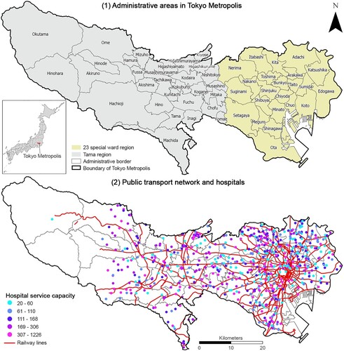
The primary goal of our study is to construct the grained-level measure of vulnerability and healthcare accessibility in Tokyo Metropolis, Japan as the most populated metropolitan region in the world (United Nations 2022) – in order to further identify the vulnerable neighbourhoods with low healthcare access and to evaluate the disparity in the built environment of vulnerable neighbourhoods. Tokyo Metropolis has a total area of 2191 square kilometres and a total population of 13.98 million in 2022 (Statistics Bureau of Japan 2022). It consists of the 23-special-ward (ku in Japanese) region towards the coast of Tokyo Bay as well as the inland Tama region that is made up of 26 cities (shi), 3 towns (machi), and 1 village (mura) (Figure 1). Drawing on multiple data sources, including the latest census data in 2022 at the level of census blocks (chome in Japanese) as the smallest statistical unit of the national census, as well as transport network, medical data, digital cadastral data, land use maps, and points of interest data retrieved from Open Street Map, our study has three research objectives to achieve: (1) measuring social vulnerability to COVID-19; (2) measuring multi-modal healthcare accessibility; and (3) evaluating the disparity in healthcare access and built environment of neighbourhoods at different levels of vulnerability. In doing so, our outcome datasets and findings provide nuanced and timely evidence for place-based health planning and policy making in the post-COVID era and beyond. Our analytical framework can be employed in other geographic contexts to help the nation better prepare for future public health crises.

Figure 1. Geographic context of Tokyo Metropolis. In addition to the 23-special-ward (ku in Japanese) region and the Tama region which is made up of 26 cities (shi), 3 towns (machi), and 1 village (mura), Tokyo Metropolis also includes the Izu Islands and the Ogasawara Islands in the Pacific Ocean, which are excluded in our study given they are geographically separated from the mainland metropolis without continuous road network connections.

2. Conceptualisation of social vulnerability to COVID-19

The definition of vulnerability has no consensus in the literature and commonly involves a number of viewpoints. The first viewpoint perceives that vulnerability as the system of being physically exposed to a crisis and exposure is usually measured by the number or density of people and buildings in hazard-affected areas (Jenelius, Petersen, and Mattsson 2006). The second viewpoint considers vulnerability as a more complex capacity of society and individuals to cope with a hazard or crisis (Flanagan et al. 2011). In this case, vulnerability often refers to social vulnerability quantified in the classic work by Cutter (1996). The latest review work by Martín and Paneque (2022) collated the vulnerability as a composite of exposure, sensitivity, and adaptive capacity however the definitions of these three elements are evolving and somehow overlapping or controversial to some degree in early studies. To narrow down the definition of vulnerability, our paper followed the second viewpoint and defined vulnerability as an adaptive capacity of society and individuals to cope with public crises (hereinafter termed social vulnerability).

We employed the Cutter’s classic framework of measuring social vulnerability (Cutter 1996) and the construction of the Social Vulnerability Index (SVI) by the US CDC (2018) to conceptualise the social vulnerability to COVID-19 and select indicators for its measurement. In the hazard-related studies, the Cutter’s classic framework defines social vulnerability as the social resistance or resilience of individuals and communities to a certain natural hazard (Cutter 1996). Such a definition can be further extended in the context of the COVID-19 pandemic where such social vulnerability indices are urgently needed in designing pandemic-specific urban environment and health planning policies, especially for communities with greater vulnerabilities. In this regard, we specify the social vulnerability to COVID-19 as the ability /capability of various groups to cope with COVID-19 and their exposure to COVID-19.

On one hand, the exposure to COVID-19 can be indicated by the density of population, buildings and/or living space (e.g. crowdedness of living) to reflect the number of victims and assets subject to public crisis/natural hazards according to the Cutter’s framework (Cutter 1996) and the Fifth Report developed by the Intergovernmental Panel on Climate Change (Estoque et al. 2020). In addition, a large body of studies have revealed that there is a positive relationship between density and viral spread (e.g. Biggs et al. 2021; Ganasegeran et al. 2021; Gerritse 2020; Selcuk, Gormus, and Guven 2021). Namely, high-density areas are more vulnerable to COVID-19 although such a relationship is complex and subject to geographic contexts with counter evidence – high-density development may not necessarily correlate to disease spread – also observed in the literature (e.g. Hamidi, Ewing, and Sabouri 2020; Gao et al. 2022; Kar et al. 2022; Khavarian-Garmsir, Sharifi, and Moradpour 2021).

On the other hand, the ability /capability of population to cope with COVID-19 is usually indicated by demographic and socioeconomic factors, such as the elderly and children, female, low income, essential work, low education, single-parent family, and housing ownership (Spielman et al. 2020). The selection of indicators varies across different geographic contexts and is also subject to data availability and local contexts. In Japan, early studies on vulnerability to COVID-19 revealed that females, and low-skilled and low-income workers were more vulnerable to COVID-19 (Kikuchi, Kitao, and Mikoshiba 2020; 2021). The U.S. CDC developed a prestigious dataset of SVI (US CDC 2018) which has been widely used in COVID-19-related studies, based on 15 indicators under four themes – (1) socioeconomic status (e.g. below poverty, unemployed, income, no high school diploma); (2) household composition & disability (e.g. aged 65 or older, aged 17 or younger, older than age 5 with a disability, single-parent households); (3) minority status & language (e.g. minority, speaking English); and (4) housing type & transportation (e.g. multi-unit structures, mobile homes, crowding, no vehicle, and group quarters).

Referring to the construction of SVI by the U.S. CDC, we select 12 indicators and the detailed justification of the expected effect of each indicator on vulnerability to COVID-19 is provided in Supplementary Table S1. A number of indicators used by the U.S. CDC are not available in Japan at the fine level, including speaking English well, vehicle ownership, education levels, disability and income due to the concern of data privacy. Alternatively, we use land prices to reflect income levels with the consideration that the land prices of properties are largely correlated with the income levels of residents (Ahlfeldt 2011; Alonso 2017); the proportion of speaking English well is the reflection of minority or migrants and such a proportion is relatively smaller in Japan compared to the major migrants-receiving countries (e.g. U.S. and Australia) (Yamashiro 2013). Although we would not be able to completely include all indicators used by the U.S. CDC, we believe that the selected 12 indicators could largely capture the ability/capacity of populations to cope with COVID-19 through careful validation from other COVID-19 data sources. To further clarify, our measures of social vulnerability to COVID-19 emphasise the social resilience and capacity of communities, rather than the physical and/or mental sensitivity of individuals to COVID-19. Thus, we do not involve health-related indicators, including the onset of chronic diseases, physical and mental conditions, and heart and vascular diseases, to name a few, which have been involved in early studies to measure health vulnerability.

3. Materials and methods

3.1. Data and the selection of indicators

We collected data from multiple sources. First, demographic and socioeconomic data were retrieved via the e-Stat – an official statistics portal developed by the Statistics Bureau of Japan (2015, 2022) at the level of census blocks (chome) as the smallest statistical unit of the national census. The latest 2022 census included population counts, age, gender, family composition, housing, migration, and living duration but did not include employment, occupation, and working style which were only available in the 2015 census (Table 1). The statistical summary of these indicators is provided in Supplementary Table S2.

Table 1. Indicators used in the measure of vulnerability.

Indicator	Detailed measurement	Definition
Age	Age above 65 (%)	People with age at or above 65over the total population
	Age 0–4 (%)	People with age at 0–4 over the total population
Gender	Female (%)	Female over the total population
Minority	Foreigner (%)	Foreigners or migrants over the total population
Family composition	Single household (%)	Households with two or more families over the total households
Income	Land price (yen/m^2)	The average land price of one census block
Employment	Unemployed (%)	Unemployed people over the total labour force
Occupation	Non-MPA (managers, professionals, and administrators) (%)	People with occupation not in manager, profession, and clerical and administration over the total labour force
Working style	Work remotely (%)	People that need to work in another ward/city over the total labour force
	Work at home (%)	People who work at home over the total labour force
Living style	Crowded living (%)	People living in middle- and high-density space (e.g. high rise apartments) over the total population
Housing ownership	Renter (%)	Renters over the total population

Second, land price data were retrieved from the Ministry of Land, Infrastructure, Transport and Tourism (2022). Given that the income level of residents was not provided in the census, we used land prices as the alternative measure to reflect income levels on the assumption that properties with higher land prices were more likely to be affordable to families/households with higher income (Ahlfeldt 2011; Alonso 2017). In this land price dataset, land prices were originally collected in 2584 survey sites spreading out the whole Tokyo Metropolis; we utilised the spatial interpolation method (detailed in ‘Methods’) to estimate income at the level of census blocks.

Third, digital cadastral and medical data were retrieved from the national land numerical information section of the Ministry of Land, Infrastructure, Transport and Tourism (2022). Medical data provided the locations of medical institutes in three types (i.e. hospitals, regular clinics and dental clinics). Considering that hospitals had inpatient facilities (e.g. beds) which were important for COVID-19 treatments while regular clinics mainly provided outpatient prescriptions and consultations to general patients, we only included hospitals (639 in the whole Tokyo Metropolis) in the measure of healthcare accessibility to ensure the computation manageable and efficient in the network analysis (detailed in ‘Methods’). In addition, hospital data had attributes (e.g. the number of beds and physicians) to reflect the medical capacity, which was used in the calculation of healthcare accessibility.

Fourth, transport network data were also retrieved from the Ministry of Land, Infrastructure, Transport and Tourism (2022). It included the network of public transit (e.g. bus routes, Tokyo Metro lines, and Japan Railway lines) as well as the network of roads with the original 19 classifications which were reclassified into two major types – drivable roads and walkable roads. Drivable roads included motorways, primary, secondary, and tertiary roads, residential streets, and trunk roads; walkable roads included additional bridleways, crossings, cycleways, elevators, escalators, footways, pedestrian paths, tracks, steps and service paths. This transport network dataset also included the attributes of connections and turns (e.g. cross-over bridges) and driving directions (e.g. one way) which were used to initiate the setting of network analysis in order to generate more realistic measures of travel routes.

Fifth, points of interest (PoI) data were retrieved from Open Street Map (OSM 2022) via OSM Application Programming Interface. The PoI dataset contained 285,187 PoI points in Tokyo Metropolis with 17 classifications – barriers (e.g. traffic signals, crossings, and motorway junctions), buildings, geological sites, leisure, military and natural sites, offices, shops, sport facilities, and tourism sites. We extracted each type of PoI to generate a total of 17 point layers which were used to quantify the built environment characteristics in ArcGIS Pro 2.8. The quantification of the built environment has been widely employed in urban research (e.g. Liu, Wang, and Xie 2019; Wang and Liu 2022) in three dimensions (i.e. design, density and diversity) or five dimensions in more recent studies (i.e. design, density, diversity, distance and destination). However, there is less consensus on which ‘D’ to be used. For example, the coverage or the access of facilities (e.g. urban parks) can be quantified as either density or the distance to the nearest facility given the high density of facilities is normally coupled with easy access; the design of streets (e.g. compact space and short blocks) can be also reflected by the density of street intersections or traffic conjunctions.

Herein, we followed the classic work by Ewing and Cervero (2010) to quantify the built environment in ‘3D’ (i.e. density, diversity and distance) with the below rationale. If the number of built environment features (e.g. buildings and amenities) are relatively large, they were quantified as ‘density’ to reflect the coverage of built environment features; if the number of built environment features (e.g. buildings and amenities) are relatively small (e.g. hospitals and museums), they were quantified as ‘distances’ to reflect the access of such facilities; for land use types, it was usually quantified as ‘diversity’ to reflect urban morphology given that the inner city areas tend to be in mixed land use while suburban areas are more likely to be dominantly residential. Specifically, the distance to the nearest PoI was calculated by the ‘near’ function; the density of PoI points in one census block was calculated by the ‘spatial joint’ function; the diversity of land use was calculated as the Simpson’s Diversity Index as detailed in Table 2.

Table 2. ‘3D’ built environment characteristics used to evaluate the disparity of areas with different levels of vulnerability.

Indicators	Definition
Distance
Distance to public facilities (m)	Distance to the nearest public facilities including government and public buildings, libraries, post offices, art galleries, and museums.
Distance to green space (m)	Distance to the nearest green space including city parks and natural parks.
Distance to cultural/historical sites (m)	Distance to the nearest cultural/historical sites including tourism sites, cultural centres, churches, temples, and historical landmarks.
Distance to water body (m)	Distance to the nearest rivers, streams, cannels, ponds and lakes.
Distance to hospitals (m)	Distance to the nearest hospitals.
Distance to public transit (m)	Distance to the nearest railway stations and bus stops.
Density
Density of amenities (per km^2)	The number of amenities over the total area of one census block, including commercial streets, shopping centres, convenience stores, pharmacies, coffee stores, restaurants and clubs.
Density of buildings (per km^2)	The number of buildings over the total area of one census block.
Density of healthcare facilities (per km^2)	The number of healthcare facilities over the total area of one census block, including hospitals, clinics, and dental clinics.
Density of recreational facilities (per km^2)	The number of recreational facilities over the total area of one census block, including leisure places, sport centres, and city parks.
Diversity
Diversity of land use (index)	The Simpson’s index for land-use diversity at the census block level, calculated as: $LUD=1-\sum {\displaystyle \frac{n_i^2}{N^2}}$, where $n_i$ = total number of areas in one census block for land use type i; N = total area of all land use types, i = types of land use classified into ten types, including commercial, education, hospital, industrial, parkland, primary production, residential, transport, water and other land use. LUD score ranges from 0 (minimum diversity) to 1 (maximum diversity).

3.2. Methods

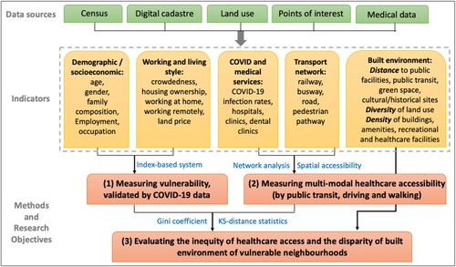
The overall analytical framework was illustrated in Figure 2. We first measured the social vulnerability index to COVID-19 by using two methods – an index-based method and a data-driven method (the principal component analysis) and validated the vulnerability metrics by COVID-19 factors. We then measured the multi-modal healthcare accessibility via network analysis and identified the areas with high vulnerability and low accessibility. Finally, the Gini coefficients and KS-distance statistics were used to evaluate the inequity of healthcare access and the disparity in the built environment of vulnerable neighbourhoods.

Figure 2. Analytical framework.

3.2.1 Estimating land prices

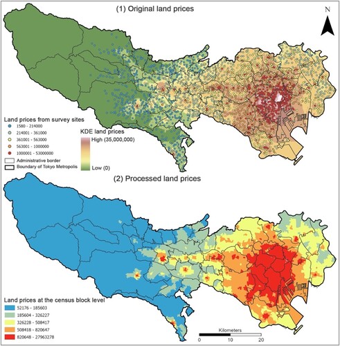
Given that income data at the level of census blocks is not available in the Japanese census, alternatively, we used land prices to reflect the income level of residents across urban space. The original land price data was collected from 2584 survey sites in Tokyo Metropolis (Figure 3(1)). We first employed the kernel density estimate (KDE), as a spatial interpolation technique, to estimate the land price at the level of census blocks based on the land price values on the 2584 survey sites. KDE was commonly used to estimate the density of spatial features within a given radius (or bandwidth) based on a kernel function (Gray and Moore 2003). Herein, we adopted the KDE function tool in ArcGIS Pro 2.8 which is built using the quartic kernel function (technical details found in ArcGIS Pro Documentation 2022). A key point for KDE is the selection of the bandwidth (Raykar and Duraiswami 2006). We defined the initial bandwidth by the tool's default calculation as the optimized option, and then checked the sensitivity of the KDE to the selection of bandwidth by increasing or decreasing the default bandwidth by 10% each time until the value reached 30% higher or lower than the default bandwidth, in order to identify the most suitable bandwidth for use to produce density estimates of land prices. Eventually, KDE generated a smooth surface raster layer of land prices covering the whole Tokyo Metropolis at the spatial resolution of 100 by 100 metres (Figure 3(2)). We then utilised the ‘zonal statistics’ function in ArcGIS Pro 2.8 to assign the land price value at the pixel level to the polygon of census blocks by the mean approach – calculating the mean of land prices of all pixels that fall into each polygon of census blocks.

Figure 3. Kernel density estimates of land prices.

3.2.2 Measuring vulnerability via an indexing approach and a principal component approach

Method 1: Following the indexing approach utilised by Atkinson and Kintrea (2001) and the selection of indicators by the US CDC (2018), we established a multi-index system to measure vulnerability based on the 12 selected indicators (Table 1). As indicated in Equation (1), the value of each indicator at the level of census blocks was compared with the whole-study-area-average value. For the indicators that were expected to have a positive relationship with vulnerability (e.g. a higher proportion of the elderly is associated with a higher level of vulnerability), if the value in one census block was lower than the whole-study-area-average value, then the index in that census block was assigned as 0 meaning that this census block has relatively a lower level of vulnerability; otherwise, it was assigned as 1 representing a higher level of vulnerability. Conversely, for the indicators that were expected to have a negative relationship with vulnerability (e.g. a lower land price is associated with a higher level of vulnerability), the index assignment in Equation (1) was reversed. In this way, we indexed each indicator and summed up the 12 indices as the overall Vulnerability Index (VI, as indicated in Eq (2)) ranging from 0 to 12, which was mapped out in ArcGIS Pro 2.8. (1) $Inde{x}_n=\{\begin{array}{c}1,if{C}_i^n>Averag{e}_i(vulnerable)\\ 0,if{C}_i^n\le Averag{e}_i(notvulnerable)\end{array}$(1) (2) $VI=\sum _{n=0}^{12}Inde{x}_n$(2) where $C_i^n$denotes the value of indicator $C$ ($n$ = 12) at the census block $i$; $Averag{e}_i$ denotes the whole-area-average value of indicator $C$ in Tokyo Metropolis.

Method 2: We also employed the principal component analysis (PCA) as the major approach widely used in the classic Cutter’s vulnerability framework (Cutter 1996) to construct the vulnerability index that was later compared with the vulnerability index generated by Method 1. PCA was commonly used to reduce data dimensions and extract the principal components that were used to construct the vulnerability index via generalising the underlying structure of input indicators (Table 1), as expressed below (Bryant and Yarnold 1995): (3) $P{C}_{block}=\sum _{i=1}^j{\displaystyle \frac{{\alpha }_i}{\sqrt{\mu }}\times X_{i,block}}$(3) where $P{C}_{block}$ denotes the principal component score for one census block; $X_{i,block}$ denotes the normalised indicator of the $i$-th indicator for the census block; ${\alpha }_i$ is the loading for the $i$-th indicator; $\mu$ denotes the eigenvalue of the principal component; $j$ is the total number of indicators in that principal component.

The procedure of PCA also includes the Kaiser-Meyer-Olkin (KMO) Test as a measure of how suited your data is for PCA. The KMO test returns values between 0 and 1. The KMO value close to 1 means the more suited the input data is to PCA. Normally a KMO value above 0.7 is acceptable in PCA (Fatoki and David 2010).

Subsequently, the PCA extracted five PCs (for the sensitivity analysis, we also extracted six to nine PCs, detailed in ‘sensitivity and validation analysis’). These five PCs were aggregated to produce an overall vulnerability index (i.e. VI in Eq. 4(4) $VI=\sum _{n=1}^{p}P{C}_{n,block}$(4) ). While some studies used different weights when aggregating the different components (e.g. Estoque et al. 2020), herein we used the evenly-weighted addition approach which has been largely employed in the Cutter’s framework (Cutter, Boruff, and Shirley 2012) and applied in different countries (e.g. Chen et al. 2013; de Loyola Hummell, Cutter, and & Emrich 2016; Guillard-Gonçalves et al. 2015; Holand, Lujala, and Rød 2011; Roncancio, Cutter, and Nardocci 2020; Wang et al., 2022b). It is easy for interpretation and justification, and not subject to arbitrary settings of weights across various contexts. Thus, the evenly-weighted addition approach to combine the PC values is as below: (4) $VI=\sum _{n=1}^{p}P{C}_{n,block}$(4) where $P{C}_{n,block}$ is the eigenvalue of that PC in one census block and $p$ is the total number of PCs extracted in that census block. Finally, the vulnerability index was normalised to range from 0 to 100 and visualised on a ten-level centile scale. A higher value of the vulnerability index close to 100 indicates a higher level of vulnerability.

3.2.3 Validation and sensitivity analysis

We conducted a series of sensitivity and validation analyses as below to decide which method to be used in the construction of vulnerability indices as well as to evaluate the confidence of such indices. First, in Method 2, we ran the PCA repeatedly to extract five to nine PCs (PCA results are provided in Supplementary Table S3 to S7) and tested whether the outcome measures of vulnerability are sensitive to the selection of PCs. Second, we compared the measures of vulnerability generated by Method 1 and 2 with COVID-19 data (e.g. COVID-19 accumulative number and infection rates) for validation purposes and then decide which method to be used. Supplementary Figure S1 displays the spatial patterns of vulnerability measures based on the extracted five to nine PCs. The pairwise Pearson’s correlation analysis (Supplementary Table S8) shows that these five measures of vulnerability are highly correlated. It means the selection of PCs does not have substantial impacts on the measures of vulnerability. Furthermore, we calculated the mean of the vulnerability measures generated by Method 1 or 2 at the ward/city level and correlated the mean values with the COVID-19 data (i.e. the accumulative number of COVID-19 cases and infection rates, visualised in Supplementary Figure S8) to decide which method is more confident to capture the near-reality vulnerability. The pairwise correlation result (Supplementary Table S8) shows that the COVID-19 accumulative numbers and infection rates are significantly correlated (p < 0.01) with the vulnerability measures generated by the indexing method (Method 1) but not correlated with ones generated by the PCA (Method 2); in addition, the COVID-19 accumulative numbers and infection rates are also significantly correlated (p < 0.01) with the percentage of high vulnerability areas over the total, the percentage of low healthcare access areas over the total, and the percentage of high vulnerability areas with low healthcare access over the high vulnerability areas (Measure 7–9 in Supplementary Table S8) – another indication that the vulnerability measures generated by the indexing approach (Method 1) are more reliable and realistic. Thus, we eventually decided to utilise the indexing approach to generate the vulnerability measures.

3.2.4 Measuring multi-modal healthcare accessibility

Existing studies in healthcare access have intensively discussed the advantages and disadvantages of methods used to measure multi-modal healthcare accessibility, including the traditional two-step floating catchment area (2SFCA) method (Luo and Wang 2003), enhanced 2SFCA (Luo and Qi 2009) and other variations of 2SFCA (e.g. Dai 2010; Dai and Wang 2011; Liu et al. 2022; Luo and Whippo 2012; McGrail and Humphreys 2014; Tao et al. 2014) which improved the traditional 2SFCA by adjusting the search radius for covering adequate supply and demand scales. Herein, we employed the friction-of-distance 2SFCA method developed by Dai (2010) in our study given it integrated the gradual distance decay effect into the traditional 2SFCA as well as functioned appropriately for large study areas (e.g. Tokyo Metropolis) and large volumes of data. The friction-of-distance 2SFCA method is implemented in two steps:

Step 1: The catchment of a hospital $j$ is defined as the area within a certain travel distance by different transport modes (e.g. by public transit, driving and walking). Then all population locations ($k$) were searched within a threshold travel zone ($h$) from a hospital location $j$ (i.e. catchment area $j$) to compute the weighted service-to-population ratio, $R_j$, within the catchment area as follows (Dai 2010): (5) $R_j={\displaystyle \frac{S_{j}F(d_{kj},h)}{{\sum }_{k\in \{d_{kj}\in h\}}{P}_k}}$(5) where $P_k$ is the total population of the census block $k$ falling within the catchment $j$ ($d_{kj}\in h$); $S_j$ is the service capacity of a hospital $j$ (e.g. the number of physicians and beds); $d_{kj}$ is the travel distance between $k$ and $j$ which was predefined to be less than the distance threshold $h$; $F(d_{kj},h)$ is the friction-of-distance function to define the distance decay effect which would be detailed further below.

Step 2: For each population location $i$, we searched all hospital locations $j$ that were within a certain travel distance threshold $h$ from the population location $i$ (i.e. catchment area $i$), and summarised the hospital-to-population ratios (calculated in Step 1), $R_j$, at these locations as follows (Dai 2010): (6) $H{A}_i^M=\sum _{j\in \{d_{ij}\in h\}}{R}_{j}F(d_{ij},h)$(6) where $H{A}_i^M$ represents the healthcare accessibility of the population at a location $i$ to hospitals using a transport mode $M$; $R_j$ is the hospital-to-population ratio at a hospital location $j$ that falls within the catchment catered at a population $i$ ($d_{ij}\in h$), and $d_{ij}$ is the travel distance between $i$ and $j$.$F(d_{ij},h)$ is the friction-of-distance function to define the distance decay effect which would be detailed further below.

To account for the distance decay between hospitals and residents, we integrated a friction-of-distance Gaussian function in the aforementioned two steps, as shown below in Equation (7). The bandwidth ($h$) in the friction-of-distance Gaussian function (Equation (8)) is the predefined travel distance threshold; namely, accessibility is decayed by travel distance proportionally towards the edge of the travel threshold, and becomes 0 beyond the distance threshold. Specifically, in the first step, the friction-of-distance Gaussian function ($F$) is used to rescale the population at each census block ($k$) according to its travel distance from hospital location ($j$). In the second step, the friction-of-distance Gaussian function ($F$) is applied to rescale $R_j$ according to the travel distance between a hospital ($j$) and a resident’s location ($i$). Accordingly, the friction-of-distance 2SFCA is written as (Dai 2010): (7) $H{A}_i^M=\sum _{j\in \{d_{ij}\in h\}}{R}_{j}F(d_{ij},h)=\sum _{j\in \{d_{ij}\in h\}}{\displaystyle \frac{S_{j}F(d_{ij},h)}{{\sum }_{k\in \{d_{kj}\in h\}}{P}_{k}F(d_{kj},h)}}$(7) (8) $F(d_{ij},h)=\{\begin{array}{c}{\displaystyle \frac{e^{-{\displaystyle \frac{1}{2}\times {\left({\displaystyle \frac{d_{ij}}{h}}\right)}^2}}-e^{-{\displaystyle \frac{1}{2}}}}{1-e^{-{\displaystyle \frac{1}{2}}}}if{d}_{ij}\le h}\\ 0if{d}_{ij}>h\end{array}$(8) where $F$ denotes the friction-of-distance Gaussian function and all other parameters are the same as in Equations (5) and (6).

Within the friction-of-distance Gaussian function, the threshold that defines the catchment area $h$ needs to be determined prior to the analysis. Herein we followed the previous studies (e.g. Apparicio et al. 2017; Higgs 2004; Mwaliko et al. 2014; Simoes and Almeida 2014; Ursulica 2016) and defined different thresholds for different transport modes – 10 km for public transit and driving, and 2km for walking. The selection of 10 and 5 km by public transit and driving was corresponding to the 40 min travel time which has been widely used as the threshold in literature (e.g. Apparicio et al. 2017; Higgs 2004; Simoes and Almeida 2014); while 2 km by walking was considered as an acceptable threshold within which people are willing to walk (Mwaliko et al. 2014; Ursulica 2016). There are a total of 5610 census blocks (as origins) and 639 hospitals (as destinations) in Tokyo Metropolis, generating a matrix containing 3,584,790 origin-destination pairs in the network analysis. After applying the distance thresholds (10km for public transit and driving, and 2km for walking), there are 2,491,121 origin-destination pairs by using public transit, 2,556,583 by driving and 224,422 by walking. Due to the large volume of data, this network analysis was conducted using arcpy.na package in Python 3.10 and the results were visualised in ArcGIS Pro 2.8. In the end, we calculated the overall healthcare accessibility as the average of three accessibility metrics for driving, walking and public transit, respectively, on the assumption that people have an equal likelihood of using three transport modes to access healthcare facilities.

3.3. Disparity analysis

We conducted a disparity analysis of areas within and across the three levels of vulnerability to COVID-19, in terms of their healthcare access (calculated in the previous step) and built environment characteristics (Table 2). We first produced a set of violin plots (Hintze and Nelson 1998) to visualise the statistics of healthcare accessibility and built environment characteristics of areas at three levels of vulnerability, including the mean, minimum and maximum, range, and frequency of the values. The horizontal width of each violin plot represents the density of selected characteristics at a certain vulnerability level; the vertical range of each violin plot indicates the range of selected characteristics at each vulnerability level.

We first utilised the Gini coefficient (Dorfman 1979) to measure the disparity in the selected built environment characteristics (e.g. density of buildings) in areas that are within each of the vulnerability categories (Dorfman 1979): (9) $Gini=1-\sum _{k=2}^n(X_k-X_{k-1})(Y_k+Y_{k-1})$(9) where $n$ is the total number of census blocks at a certain vulnerability level; k is an accumulative counter that counts up by 1 from 0 to $n$. $X_k$ is the portion of census blocks over all areas at count $k$; $Y_k$ is the portion of one selected indicator (e.g. the density of buildings) at count $k$ over the sum of that indicator of all census blocks. The value of the Gini coefficient ranges between 0 (representing total similarity) and 1 (representing total disparity).

Furthermore, we also employed the Kolmogorov–Smirnov (KS) distance statistic to measure the variation of selected indicators across areas at different levels of vulnerability. The KS distance is a nonparametric statistic to quantify the distance between the distributions of the two samples (Justel, Peña, and Zamar 1997) by taking into account the differences in both the location and shape of data distributions (Langlois et al. 2012). Hence, it can be used to reflect the similarity or disparity of selected indicators (e.g. density of buildings) across areas at different levels of vulnerability, i.e. low ($V{I}_L$), medium ($V{I}_M$), and high ($V{I}_H$). For example, for two data sub-samples, $V{I}_L=\{{\mathcal{R}}_1^{V{I}_L},{\mathcal{R}}_2^{V{I}_L},{\mathcal{R}}_3^{V{I}_L},\dots ,{\mathcal{R}}_k^{V{I}_L}\}$ with $k$ census blocks and $V{I}_H=\{{\mathcal{R}}_1^{V{I}_H},{\mathcal{R}}_2^{V{I}_H},{\mathcal{R}}_3^{V{I}_H},\dots ,{\mathcal{R}}_l^{V{I}_H}\}$ with $l$census blocks, the KS distance statistic evaluates whether $V{I}_L$ and $V{I}_H$ are drawn from the same distribution (two-sample test). The KS distance between the sets of $V{I}_L$ and $V{I}_H$, i.e. $Di{s}_{V{I}_L\leftrightarrow V{I}_H}$, is calculated as: (10) $Di{s}_{V{I}_L\leftrightarrow V{I}_H}={\left({\displaystyle \frac{kl}{k+l}}\right)}^{1/2}\underset{x}{sup}|F_{V{I}_L}(x)-F_{V{I}_H}(x)|$(10) where $F_{V{I}_L}(x)$ and $F_{V{I}_H}(x)$ denote the empirical cumulative density function (Pianosi and Wagener 2015) of set $V{I}_L$ and $V{I}_H$, respectively; $k$ denotes the number of census blocks $l$ at a certain level of vulnerability. In this study, we conducted the KS statistics based on the pairwise combination of {$V{I}_{\mathrm{L}}$, $V{I}_{\mathrm{M}}$, $V{I}_{\mathrm{H}}$}, namely, $V{I}_L\leftrightarrow V{I}_M$, $V{I}_M\leftrightarrow V{I}_H$, and $V{I}_L\leftrightarrow V{I}_H$. The set of built environment characteristics $\mathcal{R}$ are shown in Table 2.

4. Results

4.1. Spatial patterns of vulnerability to COVID-19

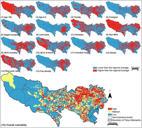
The spatial pattern of the overall vulnerability to COVID-19 is shown in Figure 4(15), with three levels of vulnerability classified in a tertile approach – low (0–33.4%), medium (33.4% to 66.7%), and high (66.7% to 100%). Areas with a high level of vulnerability mainly appear in Kita Ward, Nerima Ward and Suginami Ward in the north and northwest of the 23-special-ward region. Such highly vulnerable areas have relatively higher population density, higher proportions of the elderly, children, the unemployed, and people working in non-MPA occupations, as well as crowded living space compared to the less vulnerable areas.

Figure 4. Spatial patterns of vulnerability measures generated via the indexing approach. (1)–(14) display the spatial patterns of 14 indicators used to generate the overall vulnerability index; (15) displays the overall vulnerability measures classified at three levels – high, medium, and low – using a tertile approach.

4.2. Evaluation of healthcare access

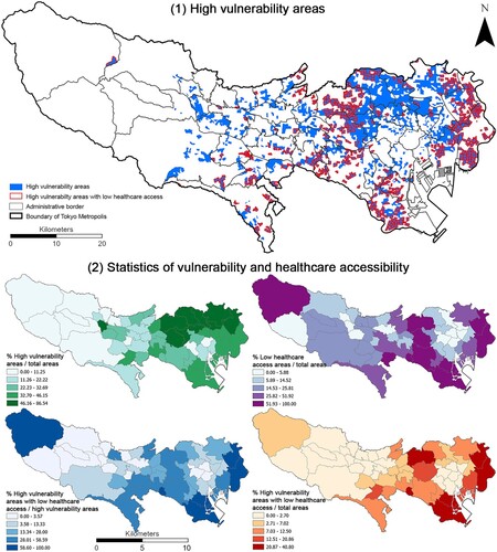
The measures of multi-modal healthcare accessibility are shown in Figure 5(1–3) by public transit, driving and walking, respectively. The overall healthcare accessibility combining the healthcare accessibility by the three types of transport modes is presented in Figure 5(4). Areas with low healthcare accessibility mainly appear in the east of the 23-special-ward region, across the border of the 23-special-ward region and the Tama region, as well as the western Tama region where there are limited numbers of hospitals and less coverage of public transit with the mountainous topography making it more difficult to travel. Figure 5(5) displays the overlay of vulnerability and healthcare accessibility, visualised in a coloured bivariate matrix. Our interest is the areas with high vulnerability and low healthcare accessibility (shown in a dark blue colour in Figure 5(5)). We further extracted the areas with high vulnerability and the areas with high vulnerability and low healthcare accessibility, as shown in Figure 6(1). They mainly appear along the border of the 23-special-ward region and Tama region (e.g. the west of Nerima Ward and Suginami Ward, the northwest of Kita Ward as well as in the east of Katsushika Ward and Edogawa Ward). Figure 6(2) shows that the proportion of highly vulnerable areas over the total is relatively higher in the north of the 23-special-ward region, including Arakawa Ward (86.54%), Kita Ward (84.07%), Nakano Ward (80%), Itabashi Ward (73.88%), Toshima Ward (68.67%), and Suginami Ward (50.36%) (statistical summary provided in Supplementary Table S3). Within these highly vulnerable areas, the proportion of areas with low healthcare access accounts for the highest in Edogawa Ward (100%), followed by Katsushika Ward (67.12%), Shinagawa Ward (66.67%), Ota Ward (65.56%), Nerima Ward (58.59%) and Setagaya Ward (46.15%) where the COVID-19 infection rate is higher than that in the central area of Tokyo and the Tama region.

Figure 5. Healthcare accessibility and vulnerability. (1) to (3) healthcare accessibility by using three transport modes (e.g. public transit, driving and walking); (4) the overall healthcare accessibility based on three transport modes; (5) overlapping healthcare accessibility and vulnerability with a bivariate legend in two dimensions – the white-pink colour ramp in the vertical form representing the three levels of accessibility and the white-blue colour ramp in the horizontal form representing the three levels of vulnerability.

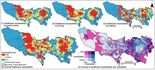
Figure 6. Delineation of areas with high vulnerability and low healthcare accessibility. (1) Location of areas with high vulnerability and low healthcare accessibility. (2) Four statistics of vulnerability and healthcare accessibility; the height of bars indicates the magnitude of percentages.

4.2.1 The disparity in healthcare access and built environment

Based on the measures of vulnerability and healthcare accessibility, we further evaluated the disparity in healthcare access and built environment of areas at each level of vulnerability (reflected by the Gini coefficient) and across different levels of vulnerability (reflected by the KS-distance statistics) (Figure 7). The statistical summary of vulnerability and healthcare accessibility is provided in Supplementary Table S4. There is less disparity in overall healthcare accessibility observed within the highly vulnerable areas (Gini coefficient = 0.25 in Figure 7(1)) compared to that within the less vulnerable areas (Gini coefficient = 0.33 and 0.51 for the medium and low level of vulnerability, respectively, in Figure 7(1)). Meanwhile, the KS-distance statistics are significant pairwise (p < 0.01) (i.e. high versus medium, medium versus low, and high versus low), indicating that healthcare accessibility is significantly different across three levels of vulnerability although such a disparity between the high and medium level of vulnerability (KS-distance = 0.07) is less obvious compared to that between the medium and low (KS-distance = 0.17) or between the high and low (KS-distance = 0.19).

Figure 7. Violin plotting of (1) the overall healthcare accessibility and (2)–(12) ‘3D’ built environment characteristics of census blocks at three levels of vulnerability. In each of the violin plots, the number along the X axis represents the Gini Coefficient for each group of census blocks in a certain level of vulnerability; the Y axis of Plot (1) represents the overall healthcare accessibility; the Y axis of Plot (2) to (7) represents the distance (km) to each type of PoI; the Y axis of Plot (8) represents the land use diversity index; the Y axis of Plot (9) to (12) represents the density of each type of PoI (counts per square km). On the top of each violin plot, three numbers represent the KS distance statistics between two groups of census blocks at different levels of vulnerability (e.g. high versus low, high versus medium, and medium versus low) at a significant level: ** p < 0.01; * p < 0.05. Within the water-drop violin bar, the vertical hollow box indicates the range (maximum and minimum) of vulnerability measures within a group. The width of water-drop areas indicates the density distribution of vulnerability measures within a group; a wider width means more spatial units (census blocks) concentrate at that level of vulnerability. The black horizontal line indicates the mean of vulnerability measures within a group. The statistical summary of vulnerability and healthcare accessibility is provided in Supplementary Table S9.

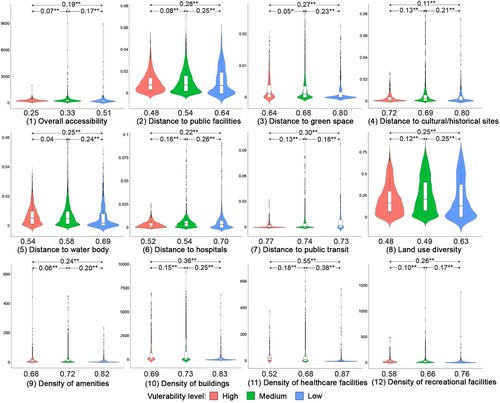
The built environment characteristics (e.g. distances to public facilities, green space, water bodies, and hospitals; land use diversity; density of amenities, buildings, healthcare and recreational facilities) display a similar pattern to the disparity in healthcare accessibility. Specifically, the disparity in the aforementioned built environment characteristics among the highly vulnerable areas is less obvious than that among the areas at low and medium levels of vulnerability; while the disparity between the high and medium levels of vulnerability is less obvious compared to that between the medium and low or between the high and low. The possible explanation is that the highly vulnerable neighbourhoods concentrate in urban areas within the 23-special-ward region (e.g. the west of Nerima Ward and Suginami Ward, the northwest of Kita Ward) where urban infrastructures and public services are fairly configurated compared to the peri-urban and rural space in the Tama region.

5. Discussion

Our study constructed the first fine-grained measures of social vulnerability to COVID-19 and healthcare accessibility in Tokyo Metropolis, Japan, delineated the highly vulnerable areas with low healthcare access, and evaluated the disparity in healthcare access and built environment of areas at different levels of vulnerability. We find that the highly vulnerable areas appear in the north, northwest and far east of the 23-special-ward region and in particular the highly vulnerable areas with low healthcare access concentrate in the west of Nerima Ward (e.g. Nakamurabashi and Oizumimachi) and Suginami Ward (e.g. Igusa and Amanuma), Itabashi Ward (e.g. Takashimadaira and Hasune), and Kita Ward (e.g. Akabane, Ukima, and Shinden) along the border between the 23-special-ward region and the Tama region as well as the north and southeast of the 23-special-ward region including Adachi Ward (e.g. Towa and Takenotsuka) and the south of Edogawa Ward (e.g. Nakakasai and Ichinoe). Such areas with high vulnerability and low healthcare access are featured by higher population density and higher proportions of the elderly, children, the unemployed, and people working in non-MPA occupations, compared to less vulnerable areas. However, the disparity in the built environment characteristics among the highly vulnerable areas is less obvious than that among the areas at low and medium levels of vulnerability, possibly because the highly vulnerable neighbourhoods concentrate in urban areas within the 23-special-ward region where infrastructures and public facilities are well configurated across urban space compared to the peri-urban and rural space in the Tama region.

Our study introduced some empirical and analytical advances in the fields of social vulnerability, healthcare access, and built environment, and provided some new insights that have not been revealed in the literature. First, we extended the concept of social vulnerability in the context of COVID-19, and generated the first fine-grained measure of vulnerability in Tokyo, Japan that can be utilised in multi-disciplinary studies in climate change, natural hazards, epidemiology, and public health. Our measure of social vulnerability to COVID-19 has a spatial pattern consistent with that revealed by Adu-Gyamfi and Shaw (2021) in disaster assessment, but turns out to be more comprehensive integrating more indicators that fit in the context of COVID-19. Second, we also produced the fine-grained measure of multi-modal healthcare accessibility by taking into account turns, driving directions, connections, and the distance-decay effect on the supply-demand ratio in the network analysis to generate a more realistic and accurate calculation of travel distances between homes and hospitals compared to the early work in the Japanese context (e.g. Du and Zhao 2022). Third, we delineated the locales with high vulnerability and low healthcare accessibility where the most efforts are needed to enhance medical resources and services. Such locales are largely concentrated in the urban space rather than rural space as revealed in existing studies (e.g, Cutter, Boruff, and Shirley 2012; Van der Ploeg et al. 2017; Wang et al., 2022a). It is possible due to that population density plays an important role in the COVID-19 viral transmission that makes high-density urban space more vulnerable than rural space (Liao et al. 2022). Fourth, the disparity in the built environment among areas at a high level of vulnerability is not substantial, aligning with the existing finding that the built environment of communities does not significantly associate with the COVID-19 viral transmission (Gao et al. 2022).

Our findings have far-reaching practical consequences for policy implications in the ongoing multi-wave COVID-19 pandemic and beyond. Our nuanced measures of social vulnerability and healthcare accessibility provide timely evidence to government and health authorities to have a latest and quantitative understanding of social resilience and socioeconomic disparities in COVID-19 outcomes in Japan which were similar to that in the U.S. and Europe (Yoshikawa and Kawachi 2021). We delineated the highly vulnerable areas and more importantly the highly vulnerable areas with low healthcare access as the locales which most need to enhance healthcare access and resources. It could guide through the future place-based health planning by prioritising the re-distribution of medical services and resources and preventing viral transmission primarily in densely populated urban space with high vulnerability. Governments and health authorities should prioritise the highly vulnerable neighbourhoods to reduce the socioeconomic inequity that has existed prior to COVID-19 but has been further exacerbated by COVID-19 (Kikuchi, Kitao, and Mikoshiba 2021). In the end, we suggest that the achievement of both socioeconomic and healthcare equity should be regarded as a post-pandemic recovery initiative that requires continuous monitoring and tracking in place-based health planning and the implementation of COVID-19-related policies.

Our study has several limitations that can be further addressed in future studies to extend our findings. First, our measures of vulnerability lack a number of indicators commonly used in other geographic contexts (e.g. income, education level, and vehicle ownership) due to data unavailability. It is possible to use the method employed in Uesugi and Asami’s work (2011) to estimate income based on other data or purchase these data from private companies in order to improve the vulnerability measure to be more robust. Second, the friction-to-distance 2SFCA method involved the distance-decay effect and predefined travel thresholds. It can be improved in future studies via surveys to reveal more realistic travel thresholds that people would bear to access healthcare facilities. Third, our analysis included hospitals – as the tertiary or secondary-level medical facilities in the Japanese healthcare system – which have the capacity and capability to provide inpatient treatments. Further efforts can be made to examine the healthcare access to primary medical facilities (e.g. general clinics and dental clinics) to improve the structure of the research on the healthcare facilities hierarchy.

6. Conclusion

With no end in sight to COVID-19, at least for now, it is crucial to reveal the latest landscape of social vulnerability and healthcare accessibility corresponding to the shift of urban-rural migration and disproportional distribution of medical resources caused by COVID-19. Meeting the urgent need of governments and public health authorities, our study contributes fine-grain measures of social vulnerability to COVID-19 and multi-modal healthcare accessibility in the post-COVID-19 era. Through the delineation of highly vulnerable neighbourhoods with low healthcare access that are most needed to enhance healthcare services in Tokyo Metropolis, Japan, our study sheds new light on the demographic and socioeconomic inequity in face of COVID-19 as well as the disparity of healthcare access and the built environment. It provides important information for place-based health planning and the smart deployment of finite health resources in a super-aging society. Moreover, it offers a practical framework to monitor and track social vulnerability and healthcare access which can be readily extended to other regions and applied to cope with future public health emergencies. We call for the joint effort from public health experts, physicians and nurses, governments and planning authorities to examine driving factors to the landscape of vulnerability and healthcare accessibility and how they shift longitudinally along the pandemic timeline. In this way, our timely evaluation of social vulnerability to COVID-19 and healthcare access can prepare us for what are bound to be new ways of living, caring, and aging in the COVID-19 era and beyond.

Disclosure statement

No potential conflict of interest was reported by the author(s).

Data availability

The COVID-19 vulnerability index and the measures of healthcare accessibility are publicly accessible via the project public repository doi:10.6084/m9.figshare.20268738.v1.

Additional information

Funding

This work was funded by the Japan Society for the Promotion of Science KAKENHI research grant (JP22F21725).

References

- Adu-Gyamfi, B., and R. Shaw. 2021. “Utilizing Population Distribution Patterns for Disaster Vulnerability Assessment: Case of Foreign Residents in the Tokyo Metropolitan Area of Japan.” International Journal of Environmental Research and Public Health 18 (8): 4061.
- Ahlfeldt, G. 2011. “If Alonso was Right: Modeling Accessibility and Explaining the Residential Land Gradient.” Journal of Regional Science 51 (2): 318–338.
- Alonso, W. 2017. “A Theory of the Urban Land Market.” In Readings in Urban Analysis, edited by William Alonso, 1–10. New York: Routledge.
- Apparicio, P., J. Gelb, A. S. Dubé, S. Kingham, L. Gauvin, and É Robitaille. 2017. “The Approaches to Measuring the Potential Spatial Access to Urban Health Services Revisited: Distance Types and Aggregation-Error Issues.” International Journal of Health Geographics 16 (1): 1–24.
- ArcGIS Pro Documentation. 2022. “Kernel Density (Spatial Analyst).” https://pro.arcgis.com/en/pro-app/2.8/tool-reference/spatial-analyst/kernel-density.htm.
- Atkinson, R., and K. Kintrea. 2001. “Disentangling Area Effects. Evidence From Deprived and Non-Deprived Neighbourhoods.” Urban Studies 38 (12): 2277–2298. doi:10.1080/00420980120087162.
- Barry, V., S. Dasgupta, D. L. Weller, J. L. Kriss, B. L. Cadwell, C. Rose, C. Pingali, et al. 2021. “Patterns in COVID-19 Vaccination Coverage, by Social Vulnerability and Urbanicity—United States, December 14, 2020–May 1, 2021.” Morbidity and Mortality Weekly Report 70 (22): 818.
- Biggs, E. N., P. M. Maloney, A. L. Rung, E. S. Peters, and W. T. Robinson. 2021. “The Relationship Between Social Vulnerability and COVID-19 Incidence among Louisiana Census Tracts.” Frontiers in Public Health 1048: 1–7.
- Bryant, F. B., and P. R. Yarnold. 1995. “Principal-components Analysis and Exploratory and Confirmatory Factor Analysis.” In Reading and Understanding Multivariate Statistics, edited by L. G. Grimm and P. R. Yarnold, 99–136. Washington, DC, USA: American Psychological Association.
- Chen, W., S. L. Cutter, C. T. Emrich, and P. Shi. 2013. “Measuring Social Vulnerability to Natural Hazards in the Yangtze River Delta Region.” China. International Journal of Disaster Risk Science 4 (4): 169–181.
- Chen, Y., S. L. Klein, B. T. Garibaldi, H. Li, C. Wu, N. M. Osevala, T. Li, J. B. Margolick, G. Pawelec, and S. X. Leng. 2021. “Aging in COVID-19: Vulnerability, Immunity and Intervention.” Ageing Research Reviews 65: 101205.
- Cutter, S. L. 1996. “Vulnerability to Environmental Hazards.” Progress in Human Geography 20 (4): 529–539.
- Cutter, S. L., B. J. Boruff, and W. L. Shirley. 2012. “Social Vulnerability to Environmental Hazards.” In Hazards Vulnerability and Environmental Justice, edited by S. L. Cutter, 143–160. London: Routledge.
- Cutter, S. L., C. T. Emrich, J. J. Webb, and D. Morath. 2009. “Social Vulnerability to Climate Variability Hazards: A Review of the Literature.” Final Report to Oxfam America 5: 1–44.
- Cutter, S. L., and C. Finch. 2008. “Temporal and Spatial Changes in Social Vulnerability to Natural Hazards.” Proceedings of the National Academy of Sciences 105 (7): 2301–2306.
- Dai, D. 2010. “Black Residential Segregation, Disparities in Spatial Access to Health Care Facilities, and Late-Stage Breast Cancer Diagnosis in Metropolitan Detroit.” Health and Place 16 (5): 1038–1052.
- Dai, D., and F. Wang. 2011. “Geographic Disparities in Accessibility to Food Stores in Southwest Mississippi.” Environment and Planning B: Planning and Design 38 (4): 659–677.
- Dailey, A. F., Z. Gant, X. Hu, S. J. Lyons, A. Okello, and A. S. Johnson. 2022. “Association Between Social Vulnerability and Rates of HIV Diagnoses Among Black Adults, by Selected Characteristics and Region of Residence—United States, 2018.” Morbidity and Mortality Weekly Report 71 (5): 167.
- Daoust, J. F. 2020. “Elderly People and Responses to COVID-19 in 27 Countries.” PloS one 15 (7): e0235590.
- DeCaprio, D., J. Gartner, T. Burgess, K. Garcia, S. Kothari, S. Sayed, and C. J. McCall. 2020. “Building a COVID-19 Vulnerability Index.” Journal of Medical Artificial Intelligence 3 (15): 20–47. doi:10.21037/jmai-20-47.
- de Loyola Hummell, B. M., S. L. Cutter, and C. T. & Emrich. 2016. “Social Vulnerability to Natural Hazards in Brazil.” International Journal of Disaster Risk Science 7 (2): 111–122.
- Dorfman, R. 1979. “A Formula for the Gini Coefficient.” The Review of Economics and Statistics 61 (1): 146–149.
- Du, M., and S. Zhao. 2022. “An Equity Evaluation on Accessibility of Primary Healthcare Facilities by Using V2SFCA Method: Taking Fukuoka City, Japan, as a Case Study.” Land 11 (5): 640.
- Estoque, R. C., M. Ooba, X. T. Seposo, T. Togawa, Y. Hijioka, K. Takahashi, and S. Nakamura. 2020. “Heat Health Risk Assessment in Philippine Cities Using Remotely Sensed Data and Social-Ecological Indicators.” Nature Communications 11 (1): 1–12.
- Ewing, R., and R. Cervero. 2010. “Travel and the Built Environment: A Meta-Analysis.” Journal of the American Planning Association 76 (3): 265–294.
- Fatoki, O., and G. David. 2010. “Obstacles to the Growth of new SMEs in South Africa: A Principal Component Analysis Approach.” African Journal of Business Management 4 (5): 729–738.
- Fekete, A. 2009. “Validation of a Social Vulnerability Index in Context to River-Floods in Germany.” Natural Hazards and Earth System Sciences 9 (2): 393–403.
- Flanagan, B. E., E. W. Gregory, E. J. Hallisey, J. L. Heitgerd, and B. Lewis. 2011. “A Social Vulnerability Index for Disaster Management.” Journal of Homeland Security and Emergency Management 8 (1): 0000102202154773551792. doi:10.2202/1547-7355.1792.
- Frigerio, I., S. Ventura, D. Strigaro, M. Mattavelli, M. De Amicis, S. Mugnano, and M. Boffi. 2016. “A GIS-Based Approach to Identify the Spatial Variability of Social Vulnerability to Seismic Hazard in Italy.” Applied Geography 74: 12–22.
- Ganasegeran, K., M. F. A. Jamil, A. S. H. Ch’ng, I. Looi, and K. M. Peariasamy. 2021. “Influence of Population Density for COVID-19 Spread in Malaysia: An Ecological Study.” International Journal of Environmental Research and Public Health 18 (18): 9866.
- Gao, Z., S. Wang, J. Gu, C. Gu, and R. Liu. 2022. “A Community-Level Study on COVID-19 Transmission and Policy Interventions in Wuhan, China.” Cities 103745.
- Gerritse, M. 2020. “Cities and COVID-19 Infections: Population Density, Transmission Speeds and Sheltering Responses.” Covid Economics 37: 1–26.
- Gray, A. G., and A. W. Moore. 2003. “Nonparametric Density Estimation: Toward Computational Tractability.” In Proceedings of the 2003 SIAM International Conference on Data Mining, edited by Daniel Barbara and Chandrika Kamath, 203–211. Philadelphia, USA: Society for Industrial and Applied Mathematics.
- Guillard-Gonçalves, C., S. L. Cutter, C. T. Emrich, and J. L. Zêzere. 2015. “Application of Social Vulnerability Index (SoVI) and Delineation of Natural Risk Zones in Greater Lisbon, Portugal.” Journal of Risk Research 18 (5): 651–674.
- Hamidi, S., R. Ewing, and S. Sabouri. 2020. “Longitudinal Analyses of the Relationship Between Development Density and the COVID-19 Morbidity and Mortality Rates: Early Evidence from 1,165 Metropolitan Counties in the United States.” Health & Place 64: 102378.
- Hawkins, R. B., E. J. Charles, and J. H. Mehaffey. 2020. “Socio-economic Status and COVID-19–Related Cases and Fatalities.” Public Health 189: 129–134.
- Higgs, G. 2004. “A Literature Review of the use of GIS-Based Measures of Access to Health Care Services.” Health Services and Outcomes Research Methodology 5 (2): 119–139.
- Hintze, J. L., and R. D. Nelson. 1998. “Violin Plots: A box Plot-Density Trace Synergism.” The American Statistician 52 (2): 181–184.
- Holand, I. S., P. Lujala, and J. K. Rød. 2011. “Social Vulnerability Assessment for Norway: A Quantitative Approach.” Norsk Geografisk Tidsskrift-Norwegian Journal of Geography 65 (1): 1–17.
- Hu, T., S. Wang, B. She, M. Zhang, X. Huang, Y. Cui, J. Khuri, et al. 2021. “Human Mobility Data in the COVID-19 Pandemic: Characteristics, Applications, and Challenges.” International Journal of Digital Earth 14 (9): 1126–1147.
- Huang, X., Z. Li, Y. Jiang, X. Ye, C. Deng, J. Zhang, and X. Li. 2021. “The Characteristics of Multi-Source Mobility Datasets and how They Reveal the Luxury Nature of Social Distancing in the US During the COVID-19 Pandemic.” International Journal of Digital Earth 14 (4): 424–442.
- Hughes, M. M., A. Wang, M. K. Grossman, E. Pun, A. Whiteman, L. Deng, E. Hallisey, et al. 2021. “County-level COVID-19 Vaccination Coverage and Social Vulnerability—United States, December 14, 2020–March 1, 2021.” Morbidity and Mortality Weekly Report 70 (12): 431.
- Jenelius, E., T. Petersen, and L.-G. Mattsson. 2006. “Importance and Exposure in Road Network Vulnerability Analysis.” Transportation Research Part A: Policy and Practice 40: 537–560.
- Justel, A., D. Peña, and R. Zamar. 1997. “A Multivariate Kolmogorov-Smirnov Test of Goodness of fit.” Statistics & Probability Letters 35 (3): 251–259.
- Kar, A., A. L. Carrel, H. J. Miller, and H. T. Le. 2022. “Public Transit Cuts During COVID-19 Compound Social Vulnerability in 22 US Cities.” Transportation Research Part D: Transport and Environment 110: 103435. doi:10.1016/j.trd.2022.103435.
- Khavarian-Garmsir, A. R., A. Sharifi, and N. Moradpour. 2021. “Are High-Density Districts More Vulnerable to the COVID-19 Pandemic?” Sustainable Cities and Society 70: 102911.
- Kikuchi, S., S. Kitao, and M. Mikoshiba. 2020. “Heterogeneous Vulnerability to the Covid-19 Crisis and Implications for Inequality in Japan.” Research Institute of Economy, Trade, and Industry (RIETI). http://www.crepe.e.u-tokyo.ac.jp/results/2020/CREPEDP71.pdf.
- Kikuchi, S., S. Kitao, and M. Mikoshiba. 2021. “Who Suffers from the COVID-19 Shocks? Labor Market Heterogeneity and Welfare Consequences in Japan.” Journal of the Japanese and International Economies 59: 101117.
- Krouse, H. J. 2020. “COVID-19 and the Widening gap in Health Inequity.” Otolaryngology–Head and Neck Surgery 163 (1): 65–66.
- Langlois, T. J., B. R. Fitzpatrick, D. V. Fairclough, C. B. Wakefield, S. A. Hesp, D. L. Mclean, E. S. Harvey, and J. J. Meeuwig. 2012. “Similarities Between Line Fishing and Baited Stereo-Video Estimations of Length-Frequency: Novel Application of Kernel Density Estimates.” PLoS One 7 (11): e45973.
- Liao, C., X. Chen, L. Zhuo, Y. Liu, H. Tao, and C. G. Burton. 2022. “Reopen Schools Safely: Simulating COVID-19 Transmission on Campus with a Contact Network Agent-Based Model.” International Journal of Digital Earth 15 (1): 381–396.
- Liu, Y., S. Wang, and B. Xie. 2019. “Evaluating the Effects of Public Transport Fare Policy Change Together with Built and Non-Built Environment Features on Ridership: The Case in South East Queensland, Australia.” Transport Policy 76: 78–89.
- Liu, L., H. Yu, J. Zhao, H. Wu, Z. Peng, and R. Wang. 2022. “Multiscale Effects of Multimodal Public Facilities Accessibility on Housing Prices Based on MGWR: A Case Study of Wuhan, China.” ISPRS International Journal of Geo-Information 11 (1): 57.
- Luo, W., and Y. Qi. 2009. “An Enhanced Two-Step Floating Catchment Area (E2SFCA) Method for Measuring Spatial Accessibility to Primary Care Physicians.” Health and Place 15 (4): 1100–1107.
- Luo, W., and F. Wang. 2003. “Measures of Spatial Accessibility to Health Care in a GIS Environment: Synthesis and a Case Study in the Chicago Region.” Environment and Planning B: Planning and Design 30 (6): 865–884.
- Luo, W., and T. Whippo. 2012. “Variable Catchment Sizes for the Two-Step Floating Catchment Area (2SFCA) Method.” Health and Place 18 (4): 789–795.
- Macias Gil, R., J. R. Marcelin, B. Zuniga-Blanco, C. Marquez, T. Mathew, and D. A. Piggott. 2020. “COVID-19 Pandemic: Disparate Health Impact on the Hispanic/Latinx Population in the United States.” The Journal of Infectious Diseases 222 (10): 1592–1595.
- Martín, Y., and P. Paneque. 2022. “Moving from Adaptation Capacities to Implementing Adaptation to Extreme Heat Events in Urban Areas of the European Union: Introducing the U-ADAPT! Research Approach.” Journal of Environmental Management 310: 114773.
- Mcgrail, M. R., and J. S. Humphreys. 2014. “Measuring Spatial Accessibility to Primary Health Care Services: Utilising Dynamic Catchment Sizes.” Applied Geography 54: 182–188.
- Ministry of Land, Infrastructure, Transport and Tourism. 2022. “National Land Numerical Information Download Service.” https://nlftp.mlit.go.jp/ksj/index.html.
- Mwaliko, E., R. Downing, W. O’Meara, D. Chelagat, A. Obala, T. Downing, C. Simiyu, et al. 2014. “Not Too far to Walk”: The Influence of Distance on Place of Delivery in a Western Kenya Health Demographic Surveillance System.”” BMC Health Services Research 14 (1): 1–9.
- Onozuka, D., and A. Hagihara. 2015. “Variation in Vulnerability to Extreme-Temperature-Related Mortality in Japan: A 40-Year Time-Series Analysis.” Environmental Research 140: 177–184.
- Open Street Map. 2022. “Data Extract.” https://openstreetmap.jp/#zoom=5&lat=38.06539&lon=139.04297&layers=000B.
- Otani, S. 2000. “Seismic Vulnerability Assessment Methods for Buildings in Japan.” Earthquake Engineering and Engineering Seismology 2 (2): 47–56.
- Pianosi, F., and T. Wagener. 2015. “A Simple and Efficient Method for Global Sensitivity Analysis Based on Cumulative Distribution Functions.” Environmental Modelling & Software 67: 1–11.
- Raykar, V. C., and R. Duraiswami. 2006. “Fast Optimal Bandwidth Selection for Kernel Density Estimation.” In Proceedings of the 2006 SIAM International Conference on Data Mining, edited by Joydeep Ghosh, Diane Lambert, David Skillicorn, and Jaideep Srivastava, 524–528. Philadelphia, USA: Society for Industrial and Applied Mathematics.
- Rimba, A. B., M. D. Setiawati, A. B. Sambah, and F. Miura. 2017. “Physical Flood Vulnerability Mapping Applying Geospatial Techniques in Okazaki City, Aichi Prefecture.” Japan Urban Science 1 (1): 7.
- Roncancio, D. J., S. L. Cutter, and A. C. Nardocci. 2020. “Social Vulnerability in Colombia.” International Journal of Disaster Risk Reduction 50: 101872.
- Schmidtlein, M. C., R. C. Deutsch, W. W. Piegorsch, and S. L. Cutter. 2008. “A Sensitivity Analysis of the Social Vulnerability Index.” Risk Analysis: An International Journal 28 (4): 1099–1114.
- Selcuk, M., S. Gormus, and M. Guven. 2021. “Impact of Weather Parameters and Population Density on the COVID-19 Transmission: Evidence from 81 Provinces of Turkey.” Earth Systems and Environment 5 (1): 87–100.
- Sha, D., Y. Liu, Q. Liu, Y. Li, Y. Tian, F. Beaini, C. Zhong, et al. 2021. “A Spatiotemporal Data Collection of Viral Cases for COVID-19 Rapid Response.” Big Earth Data 5 (1): 90–111.
- Simoes, P. P., and R. M. V. Almeida. 2014. “Maternal Mortality and Accessibility to Health Services by Means of Transit-Network Estimated Traveled Distances.” Maternal and Child Health Journal 18 (6): 1506–1511.
- Spielman, S. E., J. Tuccillo, D. C. Folch, A. Schweikert, R. Davies, N. Wood, and E. Tate. 2020. “Evaluating Social Vulnerability Indicators: Criteria and Their Application to the Social Vulnerability Index.” Natural Hazards 100 (1): 417–436.
- Statistics Bureau of Japan. 2015. “2015 Census.” https://www.e-stat.go.jp/stat-search/files?page=1&layout=datalist&toukei=00200521&tstat=000001080615&cycle=0&tclass1=000001094495&tclass2=000001094508&cycle_facet=tclass1&tclass3val=0search/files?page=1&layout=datalist&toukei=00200521&tstat=000001080615&cycle=0&tclass1=000001094495&tclass2=000001094508&cycle_facet=tclass1&tclass3val=0.
- Statistics Bureau of Japan. 2022. “2022 Census.” https://www.e-stat.go.jp/stat-search/files?page=1&layout=datalist&toukei=00200521&tstat=000001136464&cycle=0&tclass1=000001136472&tclass2=000001159886&tclass3val=0.
- Sykes, D. L., L. Holdsworth, N. Jawad, P. Gunasekera, A. H. Morice, and M. G. Crooks. 2021. “Post-COVID-19 Symptom Burden: What is Long-COVID and how Should we Manage it?” Lung 199 (2): 113–119.
- Tao, Z., Y. Cheng, T. Dai, and M. W. Rosenberg. 2014. Spatial Optimization of Residential Care Facility Locations in Beijing, China: Maximum Equity in Accessibility. International Journal of Health Geographics 13 (1): 1–11.
- Tate, E. 2012. “Social Vulnerability Indices: A Comparative Assessment Using Uncertainty and Sensitivity Analysis.” Natural Hazards 63 (2): 325–347.
- United Nations. 2022. World Cities Report 2022. https://unhabitat.org/sites/default/files/2022/06/wcr_2022.pdf.
- United States Centre of Disease Control and Prevention. 2018. CDC/ATSDR Social Vulnerability Index. https://www.atsdr.cdc.gov/placeandhealth/svi/index.html.
- Ursulica, T. E. 2016. “The Relationship Between Health Care Needs and Accessibility to Health Care Services in Botosani County-Romania.” Procedia Environmental Sciences 32: 300–310.
- Van der Ploeg, J. D., H. Renting, G. Brunori, K. Knickei, J. Mannion, T. Marsden, K. de Roest, et al. 2017. “Rural Development: From Practices and Policies Towards Theory.” In The Rural, edited by Richard Munton, 201–218. London: Routledge.
- Wang, S., and Y. Liu. 2022. “Parking in Inner Versus Outer City Spaces: Spatiotemporal Patterns of Parking Problems and Their Associations with Built Environment Features in Brisbane, Australia.” Journal of Transport Geography 98: 103261.
- Wang, S., M. Zhang, X. Huang, T. Hu, Z. Li, Q. C. Sun, and Y. Liu. 2022a. “Urban-regional Disparities in Mental Health Signals in Australia During the COVID-19 Pandemic: A Study via Twitter Data and Machine Learning Models.” Cambridge Journal of Regions, Economy and Society 1–20. https://www.researchgate.net/profile/Xiao-Huang-37/publication/361394708_Urban-regional_disparities_in_mental_health_signals_in_Australia_during_the_COVID-19_pandemic_a_study_via_Twitter_data_and_machine_learning_models/links/62add91c23f3283e3af267e2/Urban-regional-disparities-in-mental-health-signals-in-Australia-during-the-COVID-19-pandemic-a-study-via-Twitter-data-and-machine-learning-models.pdf.
- Wang, S., M. Zhang, X. Huang, T. Hu, Q. C. Sun, J. Corcoran, and Y. Liu. 2022b. “Urban–Rural Disparity of Social Vulnerability to Natural Hazards in Australia.” Scientific Reports 12 (1): 1–15.
- Yamashiro, J. H. 2013. “The Social Construction of Race and Minorities in Japan.” Sociology Compass 7 (2): 147–161.
- Yang, C., D. Sha, Q. Liu, Y. Li, H. Lan, W. W. Guan, … A. Ding. 2020. “Taking the Pulse of COVID-19: A Spatiotemporal Perspective.” International Journal of Digital Earth 13 (10): 1186–1211.
- Yoshikawa, Y., and I. Kawachi. 2021. “Association of Socioeconomic Characteristics with Disparities in COVID-19 Outcomes in Japan.” JAMA Network Open 4 (7): e2117060–e2117060.
- Zhang, M., A. Gurung, P. Anglewicz, and K. Yun. 2021. “COVID-19 and Immigrant Essential Workers: Bhutanese and Burmese Refugees in the United States.” Public Health Reports 136 (1): 117–123.