Analysis of the future trends of typical mountain glacier movements along the Sichuan-Tibet Railway based on ConvGRU network

ABSTRACT

The anomalous movements of glaciers cause disasters, such as debris flows and landslides. It is very important to assess the glacier movements and their future trends. Glacier velocity refers to movement process. The current research aims to analyse past and current spatiotemporal changes in glacier velocity. No study has used neural network model to conduct a spatiotemporal prediction for glacier velocity. Therefore, this paper selected typical mountain glaciers G2 and G5 along the Sichuan-Tibet Railway as research objects and constructed the Convolutional Gate Recurrent Unit (ConvGRU) spatiotemporal prediction model based on 1988–2018 Landsat data to predict velocities in 2019–2028, and analysed the future trends of G2 and G5. The evaluation indexes met the model requirements to a large extent, quantitatively showing that the model has high accuracy and can successfully capture the fluctuation changes in time series data of glacier velocity. The mean deviations of G2 and G5 were 0.09 and −0.47 m/yr, respectively, reflecting the high reliability of the model applied to extraction of glacier velocity. The velocities of G2 and G5 showed a slow downtrend with fluctuations; that is, they will not cause damage to the construction and operation of the Sichuan-Tibet Railway in the short term.

KEYWORDS:

• Sichuan-Tibet railway
• typical mountain glacier
• ConvGRU
• velocity
• spatiotemporal prediction

1. Introduction

As one of the key indicators of climate change, glaciers affect human life and development. Since the twentieth century, global warming has led to the retreat of glaciers in many parts of the world (Richardson and Reynolds 2000; Bolch 2007). Glaciers that were relatively stable in the past and moved relatively slowly have become more and more unstable, causing a series of glacial disasters, such as glacier surges, glacier collapses, glacial debris flows, and glacier lake outburst floods (Tian et al. 2017; Kääb et al. 2018; Tong et al. 2018). Mountain glaciers develop in high mountains and are limited by topography. Generally, they have little direct impact on human life and industrial and agricultural production but have a great impact on engineering facilities and transportation, causing massive property losses and casualties (Wu et al. 2019). Therefore, predictions of mountain glacier movements are urgently needed to analyse how future trends will evolve.

Glacier velocity reveals the glacier movement process and can quantify the differences of glacier changes (Li et al. 2013; Ding et al. 2017). It is an important parameter of the glacier dynamics model. It not only affects the mass balance, thickness, area and length changes of the glacier but also provides an important basis for the mechanism understanding and early warning of related disasters, such as glacier surges (Muhammad and Tian 2020; Zhang et al. 2021). Previous studies have used traditional observation methods to monitor glacier velocity, such as flower pole measurement and GPS measurement (Huang et al. 2014). However, there are shortcomings, such as small monitoring ranges, low efficiency, high costs and low monitoring point density (Nuimura et al. 2015; Ye et al. 2016). Most current research is based on radar images, which have the advantages of being free from cloud and rain interference and strong penetrability to obtain glacier velocity (Wang 2020). The main monitoring methods include interferometry technology and offset tracking technology. Interferometry technology uses image phase information to obtain glacier deformation but cannot effectively measure large-scale displacement due to the effect of phase decoherence between images. Offset tracking technology uses image intensity information to obtain glacier deformation, which can make up for the lack of phase decoherence and is suitable for extracting large gradient deformation (Zhang, Zhao, and Ge 2019). However, radar images are expensive. Sentinel-1A data is widely used in glacier movement monitoring due to its openness, but it was launched in 2014, making available data less. With the increase of high-performance optical remote sensing satellites, such as Landsat-8, the image data covering the glacier area is continuous, which makes it possible to carry out a long-term series study of the glacier movement process (Li et al. 2017b). The optical image based on feature matching method is similar to the radar image based on feature matching method (offset tracking technology) in nature, so the former can also be used to extract the large gradient deformation of glacier movement. However, the above monitoring methods are all used to analyse the past and current spatiotemporal changes in glacier velocity but fail to conduct spatiotemporal predictions of glacier velocity and lack an analysis of future change trends. To address these shortcomings, machine learning is the most promising technology at present. It can automatically analyse and obtain rules from data and use the rules to predict unknown data. One of its most powerful algorithms, the recurrent neural network, has been widely used in many fields. For example, Stepchenko and Chizhov (2015) used a recurrent neural network (RNN) model to predict short-term normalised difference vegetation index (NDVI), Rui, Zuo, and Li (2016) proposed a gated recurrent unit (GRU) model to predict traffic flow, and Chen et al. (2021) used a long short-term memory network (LSTM) model based on time series interferometric synthetic aperture radar (InSAR) data to predict land subsidence. The above models have achieved certain results, but the spatiotemporal changes in glacier velocity often have a neighbourhood relationship. Such models only make predictions based on the historical data of sampling points, which results in a lack of spatial neighbourhood information. Considering the ability of convolution operation to extract spatial features (Tian et al. 2020; Zhang and Han 2022) and the short time series length of the original data in this paper, we propose to use the Convolutional Gate Recurrent Unit (ConvGRU) neural network model for the spatiotemporal prediction of glacier velocity.

In the past 50 years, the Qinghai-Tibet Plateau has warmed up 0.3–0.4°C against the background of an average global warming of 0.17°C per decade, making it the region with the strongest global warming (Cui et al. 2019; Qiu et al. 2019; Wu et al. 2019; Meng et al. 2021; Duan et al. 2022). Relevant studies have pointed out that the Qinghai-Tibet Plateau and surrounding areas have shown the frequent occurrences of flood disasters caused by rapid glacier retreat, ice avalanches, landslides, debris flows, etc. (Lu et al. 2005, 2020; Bolch et al. 2012; Brun et al. 2017; An et al. 2019; Muhammad et al. 2021), most clearly in south-eastern Tibet (Song et al. 2016a; Wei et al. 2019). As a major infrastructure and livelihood project in my country, the Sichuan-Tibet Railway is located in south-eastern Tibet, and its construction and operation will be threatened and challenged by various natural disasters that may be caused by glacier movements (Cui et al. 2019).

Therefore, this paper takes the typical mountain glaciers G2 and G5 along the Sichuan-Tibet Railway as its research objects and builds a ConvGRU spatiotemporal prediction model based on interannual data on Landsat glacier velocity from 1988 to 2018 provided by the Inter-Mission Time Series of Land Ice Velocity and Elevation (ITS_LIVE) product. It obtains the prediction velocity of G2 and G5 in 2019–2028 and analyses the spatiotemporal prediction results and future trends of the two, explaining the reasons for the changes in velocity in different regions of G2 and G5 by combining factors such as the elevation, slope, branch, width of the ice tongue and ice weight of each glacier. This can provide technical support and a theoretical basis for the construction and operation of the Sichuan-Tibet Railway and provide early warnings about surrounding mountain glacier disasters.

2. Study area and data sources

2.1. Study area

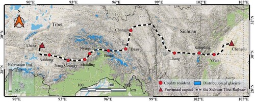
The Sichuan-Tibet Railway is a fast railway connecting Sichuan Province and the Tibet Autonomous Region in China. It runs east–west as a whole, starting from Chengdu, Sichuan Province in the east and ending in Lhasa, Tibet Autonomous Region in the west, with a total length of 1838 km. The second railway to Tibet (Jia 2021), its construction and operation are affected by various extreme geographical environments (Li, Lan, and Guo 2017a), such as mountains and hills, alpine plateaus and windy desert. The temperature differences between the regions are huge: the temperature in summer can reach 40°C, the temperature in winter can reach −20°C and the temperature difference between day and night can reach 35°C (Zhu, Jiang, and Qu 2008; Song, Zhang, and Jiang 2016b). Called ‘the most difficult railway to build’, it spans 21 snow-capped mountains over 4000 m and is constructed and operated in stages and sections (Zhang 2016; Yang 2019). The currently operating sections are the Chengya section and the Lalin section. There are mountain glaciers around the railway (Figure 1), and their distribution is particularly dense near Nyingchi and Bomê. The combination of temperature differences between day and night, rain, earthquake, strong winds and other factors will promote the rapid movement of the local surface of mountain glaciers, which will lead to a series of ice hazards, such as ice quakes, glacier debris flows and glacial lake outburst floods, creating great hidden dangers for the construction and operation of the Sichuan-Tibet railway.

Figure 1. Geographical location and topographic characteristics of the Sichuan-Tibet Railway and the mountain glaciers along the railway.

2.2. Data sources

The ITS_LIVE product comes from NASA’s MEaSUREs project (https://nsidc.org/apps/itslive/), which provides automated, low-latency global glacier velocity data over the time span of 1985–2018. This product is based on Landsat 4, 5 (1–4 bands) and Landsat 7, 8 (panchromatic bands) images and uses local normalisation, oversampling and feature tracking to extract the glacier velocity (Gardner et al. 2018). The data have good robustness and can reduce errors caused by factors such as image matching and glacier surges (Gardner, Fahnstock, and Scambos 2019; Huang, Zhang, and Zhang 2021). The research objects in this paper are typical mountain glaciers along the Sichuan-Tibet Railway, which were selected from the glacier velocity data with a spatial resolution of 240 m provided by the ITS_LIVE product. Due to the lack of glacier velocity data in 1985 and 1987 in the study area and the poor quality of glacier velocity data in 1986, we selected the glacier velocity data from 1988 to 2018.

The main idea of selecting typical mountain glaciers is to screen out the active glaciers by qualitatively and quantitatively analysing the velocity of mountain glaciers along the Sichuan-Tibet Railway in 1988–2018. The specific process is mainly as follows: (1) According to qualitative analysis, that is, using ENVI’s Raster Color Slice tool and visual interpretation, there are eight glaciers moving significantly faster along the Sichuan-Tibet Railway from 1988 to 2018, numbered G0, G1, G2, G3, G4, G5, G6 and G7, distributed in five regions A, B, C, D and E (Figure 2). (2) According to the attributes of the eight glaciers (Table 1), the areas of G2, G3 and G5 are larger, reaching 179.59, 96.28 and 128.09 km², respectively, and the slopes are gentler at 12.90°, 17.40° and 12.40°, respectively. In general, the area of a glacier is positively correlated with its ice weight, the increase in ice weight will make the glacier move faster, and the gentle slope is a favourable condition for the formation of the glacier, so the typical mountain glaciers were selected from G2, G3 and G5. (3) To further confirm the above inference, we used ArcMap to count the annual average velocity of the eight glaciers from 1988 to 2018 through quantitative analysis (Figure 3). Figure 3 shows that the annual average velocities of G2 and G5 are relatively large, at 62.84 and 51.90 m/yr, respectively, while the annual average velocity of G3 is only 36.47 m/yr. Therefore, this paper selected G2 and G5 as typical mountain glaciers along the Sichuan-Tibet railway.

Figure 2. Distribution of glaciers.

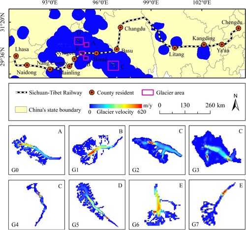
Figure 3. Annual average velocities of glaciers from 1988 to 2018.

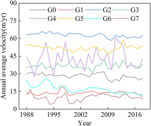
Table 1. Properties of glaciers.

FID	Area/km^2	Slope/°
0	45.97	18.00
1	37.77	27.30
2	179.59	12.90
3	96.28	17.40
4	12.42	13.80
5	128.09	12.40
6	21.90	22.60
7	18.46	26.20

In addition, 30 m resolution SRTM DEM data were selected (https://download.geoservice.dlr.de/), mainly for the analysis of the topographic characteristics of the glaciers.

3. ConvGRU network spatiotemporal prediction model of glacier movements

3.1. Dataset production

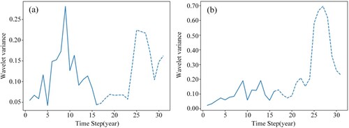
In this paper, the many-to-one prediction mode is adopted, and a sliding window is used to segment the dataset by year within all the time series data ranges. Since the time series length of the original data is short, the overlapping segmentation method is adopted to ensure a basic amount of training data. That is, a periodic analysis of the time series velocity in the typical mountain glacier area along the Sichuan-Tibet Railway is carried out using the Morlet wavelet transform (He, Yang, and Ji 2015). Figure 4 is the wavelet variance diagram of the time series velocity in typical mountain glacier areas. In Figure 4(a), it is obvious that the time step of the time series corresponding to the first peak of the G2 area is nine years; Figure 4(b) clearly shows that the time step of the time series corresponding to the first peak of the G5 area is 27 years. Considering the short time series length of the original data, if 27 years is used as a time step, the number of samples in the G5 area will be too small, resulting in overfitting and further influencing the accuracy of the ConvGRU prediction model. In addition, the second, third and fourth peaks have little difference, so the fourth peak with the shortest corresponding time step among the three is selected; that is, the time step of G5 area is also nine years. Finally, according to the Morlet wavelet transform, the time steps of typical mountain glacier areas are all nine years, which determines the length of an input time step in the production of the dataset.

Figure 4. Wavelet variance of time series velocities in typical mountain glacier areas.

The glacier velocity data provided by the ITS_LIVE product is interannual data, and the time span of the data available in this paper is 1988–2018. In the case of predicting in years, the overall dataset capacity is small. Therefore, after extracting the last five groups of data from the samples as test set labels, we divide the remaining samples into a training set (80%) and a validation set (20%) and use K-fold cross validation to divide datasets (take K = 5), obtaining K groups of training sets and validation sets. After training, the evaluation indicators of the prediction results of each model test set are finally cross-validated and the mean value is obtained.

3.2. ConvGRU network structure

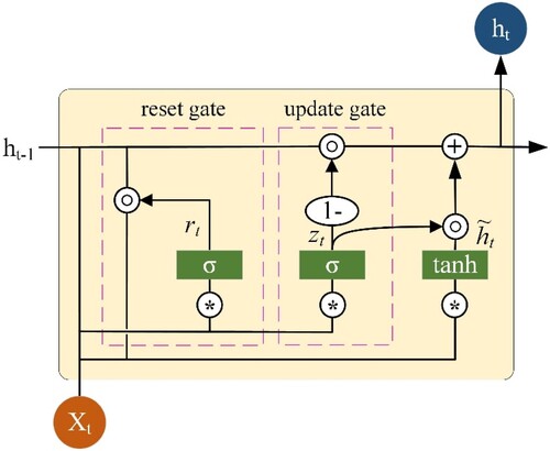
The Convolutional Gate Recurrent Unit (ConvGRU) model combines the convolutional neural network and the RNN expansion algorithm. The core idea is to add matrix operations to convolution operations, which can use not only the GRU to obtain the time series features but also the convolution calculation to extract the spatial features (Tian et al. 2020; Zhang and Han 2022). The model uses two gate structures, a reset gate and an update gate, to control the flow of information. When a new input arrives, the reset gate controls how well the previous state is cleared, and the update gate controls how well new information can be written to the current state (Shi et al. 2017). The specific calculation formulas are as follows: (1) $r_t=\sigma \left(W_r\ast \left[h_{t-1},x_t\right]+b_r\right)$(1) (2) $z_t=\sigma \left(W_z\ast \left[h_{t-1},x_t\right]+b_z\right)$(2) (3) ${\tilde{h}}_t=\tanh \left(W_{\tilde{h}}\ast \left[r_t\text{□}{h}_{t-1},x_t\right]+b_h\right)$(3) (4) $h_t=\left(1-z_t\right)h_{t-1}+z_t\text{□}{\tilde{h}}_t$(4) where, σ is a Sigmoid function that outputs the value of [0,1], tanh is a hyperbolic tangent function, $r_t$ represents the reset gate, $z_t$ represents the update gate, $\ast$ is the convolution operation □, is the Hadamard product operation, W and b are the weight matrix and bias term of different calculation processes, $h_{t-1}$is the output of the previous time step cell, $x_t$ is the input of the current cell and ${\tilde{h}}_t$ is the update information of the current cell. The network structure of a single ConvGRU cell is shown in Figure 5.

Figure 5. ConvGRU network structure.

3.3. Construction of a spatiotemporal prediction model for glacier movements

In this paper, an end-to-end network model based on a ConvGRU is proposed for spatiotemporal prediction of the time series velocity data of typical mountain glaciers along the Sichuan-Tibet Railway. The network structure is mainly divided into three parts: the encoding module, the prediction module and the decoding module. The encoder-predictor-decoder mode is used as the main frame for structural design (Figure 6).

Figure 6. Neural network model based on ConvGRU.

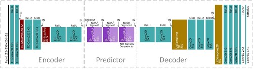
The encoding module is used to down-sampling and extract features from the glacier time series velocity data to reduce the size of the feature map, the calculation amount of the prediction module and the occupation of storage space. This module includes four scales of feature extraction, using a time distributed (TD) two-dimensional (2D) convolutional layer, a max pooling layer and an instance normalisation (IN) layer (Ulyanov, Vedaldi, and Lempitsky 2016). The size of the convolution kernel of all convolutional layers in the module is set to 3 × 3, and the feature map filling method is the same to ensure that the size of the output feature map is consistent with the current one. The output channel of the convolutional layer increases as the size of the feature map decreases. The size of the feature map is reduced from the initial 256 × 256 to 64 × 64 after two maximum pooling operations. The size of the pooling window is 2 × 2 and the step size is 2 so that the pixels are not repeatedly calculated under the premise of completely traversing all pixels and halve the width and height of the feature map.

The prediction module uses three bidirectional ConvGRU layers to perform multistep-to-one-step prediction on the time series feature map. This allows it to capture the spatiotemporal features in both positive and negative time series directions, obtain a relatively stable time series feature map and ensure the reliability of the output results to the greatest extent. The size of the convolution kernel of the three bidirectional ConvGRU layers is designed to be 3 × 3, the output channel of each time series direction is 64 and the output channel of the bidirectional time series is 128 after concat. At the same time, dropout and recurrent dropout are added to each ConvGRU layer to improve the generalisation ability of the model prediction, and the dropout ratios are all 0.25. The last ConvGRU layer does not return the full sequence but only outputs the results of the last time step cell.

The decoding module is used for up-sampling the feature map output by the prediction module to enlarge the size and restore the detailed features and output the prediction result. The feature map’s size is symmetric to the encoding module, including three progressively enlarged feature map sizes. Through the stacking of a two-dimensional convolutional layer and an up-sampling layer, the feature map sizes are gradually restored and feature details are recovered. The output channel of the convolutional layer in this module decreases with the increase of the feature map size and finally uses the four convolutional layers, whose output channel gradually decreases to 1, to reconstruct and output the glacier time series velocity data.

3.4. Model training process

The parameters of the neural network model with cyclic structure are small, but the occupation of computing resources and storage resources is relatively high in the training process. Each weight item in the ConvGRU layer in this paper is a three-dimensional matrix, which makes the resource consumption much higher than that of the traditional RNN network and requires a very high level of hardware (GPU Memory). Due to the constraints of price and the experimental environment, we pursued a balance in the experimental platform. The basic system platform configurations are shown in Table 2. In addition, important software package configurations are shown in Table 3.

Table 2. Basic system platform configurations.

Project	Operating system	CPU	Memory	Disk	GPU
Content	Microsoft Windows 10 Pro for Workstation Ver. 21H2	AMD Ryzen 9 4900HS with Radeon Graphics	16G 3200MHz	Intel 660P M.2 2280(1TB)	NVIDIA GeForce RTX 2060 with Max-Q Design GDDR6 @ 6GB (192 bits)

Table 3. Important software (package) configurations.

Project	Graphics Driver	CUDA	CUDNN	Python	Keras	Tensorflow
Content	457.63 Studio	V11.1.105	V8.1.1.33	3.7.8	2.4.0	2.4.1

By comprehensively considering the computational efficiency, result accuracy and hardware conditions of the model, this paper sets the number of iterations to 64 and the batch size to 2. The optimiser uses adaptive moment estimation (Adam) (Kingma and Ba 2015), and the initial learning rate is set to 5.0 × 10⁻⁵. Considering the large shape of the temporary feature map during the calculation process, a half-precision (16 bits) floating-point format is used for training. At the same time, the callback function is set to monitor so that when the loss of the validation set does not decrease for eight consecutive epochs, the learning rate decreases to 10% of the current value. The metric is structural similarity (SSIM), and the custom loss function is the weighted sum of the mean absolute error (MAE), SSIM and the peak signal-to-noise ratio (PSNR). The mathematical expression of the loss function is as follows: (11) $Loss=W_{\mathrm{M}\mathrm{A}\mathrm{E}}\times \mathrm{M}\mathrm{A}\mathrm{E}+W_{\mathrm{S}\mathrm{S}\mathrm{I}\mathrm{M}}\times \left(1-\mathrm{S}\mathrm{S}\mathrm{I}\mathrm{M}\right)+W_{\mathrm{P}\mathrm{S}\mathrm{N}\mathrm{R}}\times \left(1-\mathrm{P}\mathrm{S}\mathrm{N}\mathrm{R}/100\right)$(11) here, $W_{\mathrm{M}\mathrm{A}\mathrm{E}}$,$W_{\mathrm{S}\mathrm{S}\mathrm{I}\mathrm{M}}$ and $W_{\mathrm{P}\mathrm{S}\mathrm{N}\mathrm{R}}$ are the weights of MAE, SSIM and PSNR, respectively. $W_{\mathrm{M}\mathrm{A}\mathrm{E}}$ = 0.4, $W_{\mathrm{S}\mathrm{S}\mathrm{I}\mathrm{M}}$ = 0.4 and $W_{\mathrm{P}\mathrm{S}\mathrm{N}\mathrm{R}}$ = 0.2 are the settings for this experiment.

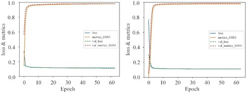
After 64 epochs on the training set, the network finally approximated convergence. The many-to-one network model of G2 and G5 at different time steps obtained structural similarities of about 0.980 and 0.979 on the training set, respectively, and about 0.981 and 0.984 on the validation set, respectively. The index changes during the training process are shown in Figure 7.

Figure 7. Metric changes of G2 and G5 during training.

3.5. Evaluation index

To quantitatively evaluate the performance of the constructed ConvGRU network glacier movement spatiotemporal prediction model, the following indicators were used to evaluate the spatiotemporal prediction accuracy of the output results: the mean absolute error (MAE), mean squared logarithmic error (MLSE), coefficient of determination (R²), explained var score (EVar), structural similarity (SSIM) (Wang, Bovik, and Sheikh 2004), and peak signal-to-noise ratio (PSNR) (Huynh-Thu and Ghanbari 2008).

MAE: (5) $MAE={\displaystyle \frac{1}{n}\sum _{i=1}^n\left|y_i-{\hat{y}}_i\right|}$(5)

MLSE: (6) $MLSE={\displaystyle \frac{1}{n}\sum _{i=1}^n(\log ({\hat{y}}_i+1)-\mathrm{l}\mathrm{o}\mathrm{g}(y_i+1){)}^2}$(6)

R²: (7) $R^2=1-{\displaystyle \frac{{\sum }_{i=1}^n{\left(y_i-{\hat{y}}_i\right)}^2}{{\sum }_{i=1}^n{\left(y_i-{\overline{y}}_i\right)}^2}}$(7) EVar: (8) $EVar=1-{\displaystyle \frac{{\sum }_{i=1}^n{\left(y_i-{\hat{y}}_i-\left(\overline{y}-\overline{\hat{y}}\right)\right)}^2}{{\sum }_{i=1}^n{\left(y_i-{\overline{y}}_i\right)}^2}}$(8)

SSIM: (9) $SSIM\left(x,y\right)={\displaystyle \frac{\left[2{\mu }_x{\mu }_y+{\left(k_{1}L\right)}^2\right]\left[2{\sigma }_{xy}+{\left(k_{2}L\right)}^2\right]}{\left[{\mu }_x^2+{\mu }_y^2+{\left(k_{1}L\right)}^2\right]\left[{\sigma }_x^2+{\sigma }_y^2+{\left(k_{2}L\right)}^2\right]}}$(9) PSNR: (10) $PSNR=10\times {\log }_{10}\left[{\displaystyle \frac{{\left(2^n-1\right)}^2}{{\displaystyle \frac{1}{n}{\sum }_{i=1}^n\left|y_i-{\hat{y}}_i\right|}}}\right]$(10)

In the above formulas, $y_i$ is the real value, ${\hat{y}}_i$ is the predicted value, ${\overline{y}}_i$ is the average value, $n$ is the number of test sets, ${\mu }_x$ and ${\mu }_y$ are the average of two images, ${\sigma }_x^2$ and ${\sigma }_y^2$ are the variance of two images, ${\sigma }_{xy}$ is the covariance of two images, $L$ is the dynamic range of the pixel values and $k_1$ and $k_2$ are two scalar constants, which are $k_1$ = 0.01 and $k_2$ = 0.03 default.

4. Results and analysis

4.1. Spatiotemporal prediction results of typical mountain glacier movements

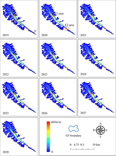
Figures 8 and 9 display the prediction results of the typical mountain glaciers time series velocities obtained using the ConvGRU model. It can be observed that the change trend of the velocity of the glaciers in the prediction period from 2019 to 2028 is consistent, and there are high-speed areas: E area of G2, E1 area and E2 area of G5. The annual average velocities of G2 and G5 are 61.47 and 48.46 m/yr, respectively.

Figure 8. Prediction results of time series velocities of G2.

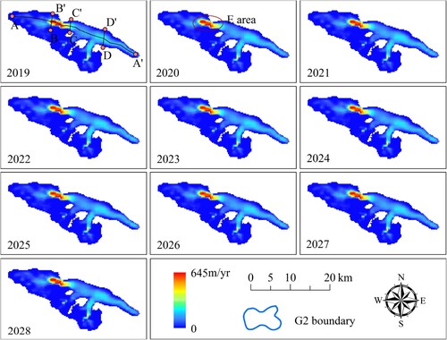
Figure 9. Prediction results of time series velocities of G5.

4.2. Analysis and future trends of spatiotemporal prediction results of typical mountain glacier movements

The glacier movement process is very complex, and the velocity of the mainstream line can roughly reflect the overall movement state of the glacier. We use ArcMap software to obtain the velocity of the mainstream line. The specific process is as follows: (1) Create a new vector of line type and define its geographic coordinate system; (2) Use the Editor tool to draw the vector and it is the vector of the mainstream line; (3) Obtain the value of the vector of the mainstream line on the glacier velocity by linear interpolation, which is the velocity of the mainstream line. To analyse the spatiotemporal prediction results of G2 and G5 in detail, this paper extracts the velocity of the mainstream line (AA’) (Figure 10) and three cross-section lines (BB’, CC’ and DD’) (Figure 11) with the changes in elevation and slope from 2019 to 2028.

Figure 10. Velocities of the mainstream line (AA’) of typical mountain glaciers in elevation and slope.

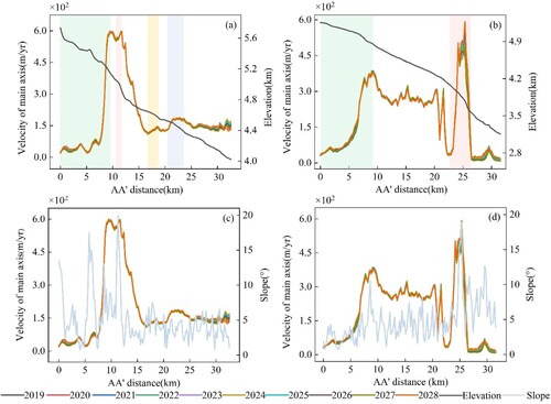
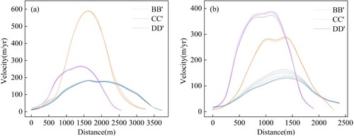
Figure 11. Velocities of cross-section lines (BB’, CC’ and DD’) of typical mountain glaciers.

Figure 10 clearly shows that the velocity of the mainstream line (AA’) of G2 and G5 decreases as the elevation decreases; with the changes in the slope, the velocity of the mainstream line (AA’) of G2 and G5 shows a consistent fluctuation. Figure 10(a) and (b) show that the elevation of G2 gradually decreases from about 5,733 m to about 4,023 m along the mainstream line (AA’), and the annual average velocity of the mainstream line (AA’) varies from around 22 m/yr to around 596 m/yr; The elevation of G5 gradually decreases from about 5,257 m to about 3,158 m along the mainstream line (AA’), and the annual average velocity of the mainstream line (AA’) varies from about 13 m/yr to about 518 m/yr. Figure 10(c) and (d) show that the slope of G2 varies from about 0.70° to about 23.51°along the mainstream line (AA’), and the slope of G5 varies from about 0.72° to 18.85° along the mainstream line (AA’). In addition, according to the local increase in mainstream line (AA’) velocity of G2 and G5 at different distances along the mainstream line shown in Figure 10, we show the velocity increase positions of G2 in Figure 10(a) with green, red, yellow and blue rectangles, which are between 0–9.51 km, 10.68–11.56 km, 16.49–18.73 km and 20.53–23.67 km along the mainstream line (AA’), respectively; In Figure 10(b), the green rectangle and the red rectangle show the velocity increase positions of G5, which are between 0–9.03 km and 22.84–26.02 km along the mainstream line (AA’), respectively.

Figure 11(a) shows that the maximum annual average velocities of the cross-section lines BB’, CC’ and DD’ of G2 can reach 589.31, 264.98 and 182.29 m/yr, respectively. Figure 11(b) shows that the maximum annual average velocities of cross-section lines BB’, CC’ and DD’ of G5 can reach 281.99, 374.01 and 141.95 m/yr, respectively. In Figure 11, it can be clearly seen that the edge velocity on both sides of G2 and G5 is near 0 m/yr, and compared with G2, the velocity of G5’s three cross-section lines in 2019–2028 fluctuates more, especially the velocity of cross-section line DD’. In addition, the velocities of the three cross-section lines (BB’, CC’ and DD’) of G2 and G5 from 2019 to 2028 are all fast in the middle and slow on the two sides, which is in line with the movement law of glaciers (Huang and Sun 1982); that is, the velocity decreases from the mainstream line of the glacier to the edges on both sides.

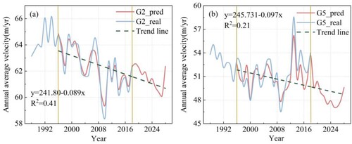
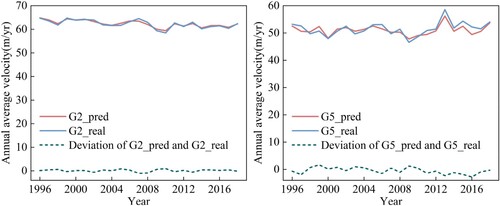
In addition, by comparing the real annual average velocities of typical mountain glaciers G2 and G5 in 1988–2018 with their predicted annual average velocities in 2019–2028 (Figure 12), it is obvious that the overall velocities of both show obvious fluctuations. Figure 12(a) shows that the maximum values of the real value and the predicted value of G2 from 1996 to 2018 are 64.72 and 64.85 m/yr, respectively, and the minimum values are 58.48 and 59.43 m/yr, respectively, and the calculated reduction rates of the real values and predicted values are 5.06% and 4.36%, respectively; Figure 12(b) shows that the maximum values of the real value and predicted value of G5 from 1996 to 2018 are 58.57 and 56.21 m/yr, respectively, and the minimum values are 46.58 and 47.83 m/yr, respectively, and the calculated reduction rates of the real values and predicted values are 11.40% and 8.06%, respectively; That is, the difference between the reduction rates obtained from the real values and predicted values is small, with an average of about 2%, which proves that the curve-fitting effect of the real value and the predicted value of the two is good. In addition, quantitative analysis shows that the annual average velocities of G2 and G5 have a slow decreasing trend. By linearly fitting the predicted annual average velocities of G2 and G5, it is found that the slopes of the trend lines of both are negative, which further proves that, with the passage of time, the annual average velocities of both show a downward trend. In summary, the movements of G2 and G5 show a slow downtrend with fluctuations as a whole.

Figure 12. Comparison of the real values and the predicted values.

5. Discussions

5.1. Model accuracy analysis

Table 4 shows the performance of the test set output of the ConvGRU-based spatiotemporal prediction model on various evaluation indexes. In general, the smaller the values of MAE and MLSE, the closer R², EVar and SSIM are to 1, and the closer PSNR is to 40 dB, the better the model’s predictive effect is. The table below clearly displays that the MAE and MLSE of the typical mountain glaciers G2 and G5 along the Sichuan-Tibet Railway are all small; R², EVar and SSIM are all large, and above 0.9; the PSNR approaches 40 dB, which quantitatively shows that the constructed ConvGRU model has high accuracy and can successfully capture the fluctuations of glacier velocity time series data.

Table 4. Evaluation indexes.

	MAE	MSLE	R^2	EVar	SSIM	PSNR
G2	2.036532	0.247138	0.93174	0.932381	0.969578	38.83055
G5	2.259422	0.338053	0.908992	0.909312	0.946173	38.91

In addition, in order to visually verify the reliability of the ConvRGU-based spatiotemporal prediction model for extracting the velocity of typical mountain glaciers G2 and G5 along the Sichuan-Tibet Railway, this paper makes the difference between the real value and predicted value of the two from 1996 to 2018 (Figure 13), it is found that the deviations of the two are both around 0 m/yr, and the mean deviations are 0.09 and −0.47 m/yr, respectively. Compared with the annual average velocity of G2 and G5, the deviations of the two are negligible. It reflects the high reliability of the spatiotemporal prediction model based on ConvRGU applied to the extraction of glacier velocity.

Figure 13. Deviations between the real values and the predicted values.

5.2. Analysis on influencing factors of typical mountain glacier movement

Figure 11 shows that the velocity fluctuations of three cross-section lines (BB’, CC’ and DD’) in G5 from 2019 to 2028 are larger than those of G2, especially the velocity of the cross-section line DD’. It is speculated that this may be related to the width of the glacier tongue and the branches of the glacier (Li et al. 2014). The narrower the ice tongue and the more branches, the more susceptible the glacier velocity is to fluctuations. Combining Figures 9 and 10, it can be seen that G5 has more branches than G2 and its ice tongue is narrower than that of G2, becoming narrower and narrower along the mainstream line (AA’), resulting in the velocities of the cross-section lines (BB’, CC’ and DD’) of G5 being more susceptible to the influx of branch velocity. As a result, the velocity fluctuations of the cross-section lines (BB’, CC’ and DD’) along the mainstream line (AA’) become larger and larger, especially the velocity of cross-section line DD’. In addition, the velocities of the cross-section lines (BB’, CC’ and DD’) of G2 and G5 decrease from the mainstream line of the glacier to the edges on both sides, mainly because the velocity on both sides is affected by the friction of mountains on both sides (Zhang, Zhao, and Ge 2019). The closer to both sides, the greater the friction of the mountain, and the closer the velocity is to 0 m/yr.

Figure 10 shows that the velocities of G2 and G5 along the mainstream line (AA’) are quite different, which is mainly related to factors such as ice weight, elevation difference and slope (Zhou, Zhen, and Guo 2014). In general, increases in ice weight, elevation and slope increase the velocity of glacier movement. The glacial ice in fim-basin starts to move when its own gravity is greater than the ground friction, which explains the gradual increase in velocity in the green rectangle area in Figure 10(a) and (b). In addition, Figure 10(a) and (b) show that the distance between the mainstream lines (AA’) of G2 and G5 is about 30 km, but the elevations at the corresponding distances are very different, showing that the overall elevation of G2 is higher than that of G5. Moreover, according to Table 3, the areas of G2 and G5 are 179.59 and 128.09 km², respectively; that is, the area of G2 is 51.50 km² larger than that of G5, which means that the velocity of glacial ice in the G2 fim-basin area at a distance of about 10 km along the mainstream line (AA’) is about 214 m/yr greater than that of G5. With the continuous movement of the glacier, the ice weight gradually decreases, the friction force gradually increases and the glacier velocity begins to decrease. However, Figure 10(a) shows that G2 has three obvious local increase areas during the decrease in glacier velocity, which are marked with red, yellow and blue rectangles, respectively. Figure 10(b) shows that there is a relatively obvious local increase area in G5 in the process of glacier velocity reduction, which is marked with a red rectangle. Combined with Figure 10(c) and (d), it is found that this phenomenon is closely related to the elevation and slope. It can be seen from the calculation that the elevation differences of the red, yellow and blue rectangular areas of G2 are close to 139, 82 and 144 m, respectively, and the distances along the mainstream line (AA’) are close to 0.88, 2.24 and 3.14 km, respectively. It is concluded that when the distances between the mainstream line in each region is certain, both are 0.88 km, the elevation differences of the red, yellow and blue rectangular areas are 139, 32 and 40 m, respectively. That is, the elevation difference of the red rectangular area is the largest, and the slope fluctuation in this area is also the largest, and the difference between the maximum and minimum values is 18.28°. Therefore, the main reasons for the increase in the velocity in the red rectangular area of G2 are the high elevation, large elevation difference and sudden increase in slope, while the yellow and blue rectangular areas have low elevations and small elevation differences. The change in slope is the main reason for the slow increase in velocity in the two regions. The increase in velocity in the red rectangular area of G5 is inseparable from the narrowing of the ice tongue and the influence of more branches. In addition, the slope in this area has the largest fluctuation range and the difference between the maximum and minimum values is 16.28°, which makes the velocity increase sharply.

6. Conclusions

Based on the glacier velocity data provided by the ITS_LIVE product, this paper qualitatively and quantitatively analysed the velocity of mountain glaciers along the Sichuan-Tibet Railway from 1988 to 2018, screened out G2 and G5 as typical mountain glaciers. It built a ConvGRU spatiotemporal prediction model to conduct velocity predictions from 2019 to 2028 of G2 and G5, analysed the spatiotemporal prediction results and future trends of the two and explained the reasons for the changes in velocity in different regions of G2 and G5 by combining factors such as the elevation, slope, branch, width of the ice tongue, and ice weight of the glacier. The following conclusions are drawn: the results of each evaluation index were in line with the model requirements to a large extent, which quantitatively shows that the constructed ConvGRU model has high accuracy and can successfully capture the fluctuation in the glacier velocity time series data. At the same time, by calculating the deviation between the real values and the predicted values of G2 and G5, it can be seen that the mean deviations are 0.09 and −0.47 m/yr, respectively, which are negligible, reflecting the high reliability of the application of the ConvRGU-based spatiotemporal prediction model to the extraction of glacier velocity. The mainstream line (AA’) velocity of G2 and G5 gradually decreases with the decrease in elevation and fluctuates in line with the change in slope. The large difference in velocity is mainly related to factors such as ice weight, elevation difference and slope. In general, the increase in ice weight, elevation and slope will speed up the velocity of the glacier; the velocities of cross-section lines (BB’, CC’ and DD’) decrease from the axis to the edges on both sides because the velocities at the edges on both sides are affected by the friction of the two sides of the mountain. The velocity fluctuations of the cross-sections (BB’, CC’ and DD’) of G5 are larger than that of G2, especially the velocity of cross-section DD’, which is mainly related to the width of the glacier tongue and the branches of the glacier. The narrower the ice tongue and the more numerous branches, the more susceptible the glacier velocity is to fluctuations. Comparing the real annual average velocities of G2 and G5 in 1988–2018 and the predicted annual average velocities in 2019–2028, it is found that the overall velocities of both show obvious fluctuations. It is calculated that the average reduction rate of the real value and the predicted value of G2 and G5 in 1996–2018 is about 2%, and the predicted annual average velocities of G2 and G5 are linearly fitted to find that the slopes of the trend lines are all negative, indicating that the annual average velocities of the glaciers have a slow decreasing trend. That is, in general, the overall movement velocities of G2 and G5 show a slow downtrend with fluctuations, which will not cause harm to the construction and operation of the Sichuan-Tibet Railway in the short term.

In this paper, the ConvRGU model is constructed based on Landsat glacier velocity interannual data to conduct a spatiotemporal prediction for the velocity of typical mountain glaciers along the Sichuan-Tibet Railway. Quantitative analysis of the movement results of G2 and G5 shows that the prediction results conform to the law of glacier movement, indicating that the model can be successfully applied to the future trend analysis of glacier movement. This has important practical significance for the safe operation of the Sichuan-Tibet Railway and the normal production and life of residents in the region. However, our prediction is data-driven, and there is a lack of sufficient research on the mechanism that affects the glacier velocity. In addition, there are few factors to consider when analysing the spatiotemporal prediction results of G2 and G5, and only ice weight, the branches of the glacier, the width of the glacier tongue, elevation and slope are involved. Future research will take into account more comprehensively the influencing factors of glacier velocity, such as temperature and precipitation. Because the velocities of different glaciers vary greatly, the more factors involved, the more likely we are to find the main factors affecting the movement of specific glaciers.

Acknowledgments

The authors thank the support from the ITS_LIVE product coming from NASA’s MEaSUREs project to provide automated, low-latency global glacier velocity data.

Disclosure statement

No potential conflict of interest was reported by the author(s).

Data availability statement

The data that support the findings of this study are available from the corresponding author upon reasonable request.

Additional information

Funding

This work was supported by the National Scientific Foundation of China [grant number 42161063]; Open Foundation of Key Laboratory of Yellow River Water Environment in Gansu Province [grant number 121YRWEK001]; Science and Technology Plan of Gansu Province [grant number 20JR2RA002]; Natural Science Foundation of Gansu Province [grant number 20JR10RA249]; Youth Science and Technology Foundation of Gansu Province [grant number 20JR10RA272]; Lanzhou Jiaotong University-Tianjin University Innovation Project Fund Project [grant number 2020055]; Jiayuguan City 2021 Science and Technology Plan Projects [grant number 21-35].

References

- An, G., L. Han, S. Huang, Y. Gu, Z. Guo, and S. Wang. 2019. “Dynamic Variation of Glaciers in Nyainqentanglha Mountain During 1999-2015: Evidence from Remote Sensing.” Geoscience 33 (1): 176–186.
- Bolch, T. 2007. “Climate Change and Glacier Retreat in Northern Tien Shan (Kazakhstan/Kyrgyzstan) Using Remote Sensing Data.” Global and Planetary Change 56 (1/2): 1–12.
- Bolch, T., A. Kulkarni, A. Kääb, C. Huggel, F. Paul, J. Cogley, H. Frey, et al. 2012. “The State and Fate of Himalayan Glaciers.” Science 336: 310–314.
- Brun, F., E. Berthier, P. Wagnon, A. Kääb, and D. Treichler. 2017. “A Spatially Resolved Estimate of High Mountain Asia Glacier Mass Balances from 2000 to 2016.” Nature Geoscience 10: 668–675.
- Chen, Y., Y. He, L. Zhang, Y. Chen, H. Pu, and B. Chen. 2021. “Prediction of InSAR Deformation Time-Series Using a Long Short-Term Memory Neural Network.” International Journal of Remote Sensing 42 (18): 6921–6944.
- Cui, P., X. Guo, T. Jiang, G. Zhang, and W. Jin. 2019. “Disaster Effect Induced by Asian Water Tower Change and Mitigation Strategies.” Bulletin of Chinese Academy of Sciences 34 (11): 1313–1321.
- Ding, Y., X. Cheng, C. Cheng, and F. Hui. 2017. “Monitoring ice Velocity by SAR Offset-Tracking and Analysis of Influence Factors for the Kangshung Glacier in the Tibetan Plateau.” Chinese Journal of Geophysics 60 (05): 1650–1658.
- Duan, A., S. Liu, W. Hu, D. Hu, and Y. Peng. 2022. “Long-term Daily Dataset of Surface Sensible Heat Flux and Latent Heat Release Over the Tibetan Plateau Based on Routine Meteorological Observations.” Big Earth Data, 1–12. doi:10.1080/20964471.2022.2037203.
- Gardner, A., M. Fahnstock, and T. Scambos. 2019. “ITS_LIVE Regional Glacier and Ice Sheet Surface Velocities: Version 1.” Data archived at National Snow and Ice Data Center. doi:10.5067/6II6VW8LLWJ7.
- Gardner, A., G. Moholdt, T. Scambos, M. Fahnstock, S. Ligtenberg, M. Broeke, and J. Nilsson. 2018. “Increased West Antarctic and Unchanged East Antarctic ice Discharge Over the Last 7 Years.” Cryosphere Discussions 12 (2): 521–547.
- He, Y., T. Yang, and Q. Ji. 2015. “Glacier Variation and Motivation Based on Remote Sensing Data in the Central Asia Alatau Regions.” Mountain Research 33 (02): 148–156.
- Huang, L., Z. Li, J. Zhou, and B. Tian. 2014. “Glacier Change Monitoring Using SAR: An Overview.” Advances in Earth Science 09: 985–994.
- Huang, M., and Z. Sun. 1982. “Some Characteristics of Continental Glacier Movement in my Country.” Journal of Glaciology and Geocryology 02: 35–46.
- Huang, D., Z. Zhang, and S. Zhang. 2021. “Characteristics of Glacier Movement in the Eastern Pamir Plateau.” Arid Land Geography 44 (1): 131–140.
- Huynh-Thu, Q., and M. Ghanbari. 2008. “Scope of Validity of PSNR in Image/Video Quality Assessment.” Electronics Letters 44 (13): 800–801.
- Jia, C. 2021. “Hazard Assessment and Zoning Research of Landslide in Tianquan Section of Sichuan-Tibet Railway Based on GIS.” Msc thesis., Southwest Jiaotong University.
- Kääb, A., S. Leinss, A. Gilbert, Y. Bühler, S. Gascoin, S. Evans, P. Bartelt, et al. 2018. “Massive Collapse of two Glaciers in Western Tibet in 2016 After Surge-Like Instability.” Nature Geoscience 11 (2): 114–120.
- Kingma, D., and J. Ba. 2015. “Adam: A Method for Stochastic Optimization.” e-prints: arXiv:1412.6980. https://ui.adsabs.harvard.edu/abs/2014arXiv1412.6980 K.
- Li, L., H. Lan, and C. Guo. 2017a. “Geohazard Susceptibility Assessment Along the Sichuan-Tibet Railway and its Adjacent Area Using an Improved Frequency Ratio Method.” Geoscience 31 (05): 911–929.
- Li, J., Z. Li, X. Ding, Q. Wang, J. Zhu, and C. Wang. 2014. “Investigating Mountain Glacier Motion with the Method of SAR Intensity-Tracking: Removal of Topographic Effects and Analysis of the Dynamic Patterns.” Earth-Science Reviews 138: 179–195.
- Li, J., Z. Li, C. Wang, J. Zhu, and X. Ding. 2013. “Using SAR Offset-Tracking Approach to Estimate Surface Motion of the South Inylchek Glacier in Tianshan.” Chinese Journal of Geophysics 56 (04): 1226–1236.
- Li, Y., S. Yan, Z. Li, H. Zhou, Y. Zheng, and X. Liu. 2017b. “The Flow State of South Inylchek Glacier in the Tianshan Mountains in 2016: Extraction and Analysis Based on Landsat-8 OLI Image.” Journal of Glaciology and Geocryology 39 (6): 1281–1288.
- Lu, J., Y. Qiu, X. Wang, W. Liang, P. Xie, L. Shi, M. Menenti, and D. Zhang. 2020. “Constructing Dataset of Classified Drainage Areas Based on Surface Water-Supply Patterns in High Mountain Asia.” Big Earth Data 4 (3): 225–241. doi:10.1080/20964471.2020.1766180.
- Lu, A., T. Yao, L. Wang, S. Liu, and Z. Guo. 2005. “Study on the Fluctuations of Typical Glaciers and Lakes in the Tibetan Plateau Using Remote Sensing.” Journal of Glaciology and Geocryology 06: 783–792.
- Meng, F., L. Huang, A. Chen, Y. Zhang, and S. Piao. 2021. “Spring and Autumn Phenology Across the Tibetan Plateau Inferred from Normalized Difference Vegetation Index and Solar-Induced Chlorophyll Fluorescence.” Big Earth Data 5 (2): 182–200. doi:10.1080/20964471.2021.1920661.
- Muhammad, S., L. Jia, F. Jakob, S. Finu, M. Ghulam, B. Etienne, L. Guo, L. Wu, and L. Tian. 2021. “A Holistic View of Shisper Glacier Surge and Outburst Floods: From Physical Processes to Downstream Impacts.” Geomatics, Natural Hazards and Risk 12 (1): 2755–2775.
- Muhammad, S., and L. Tian. 2020. “Mass Balance and a Glacier Surge of Guliya ice cap in the Western Kunlun Shan Between 2005 and 2015.” Remote Sensing of Environment 244: 111832.
- Nuimura, T., A. Sakai, K. Taniguchi, H. Nagai, D. Lamsal, S. Tsutaki, A. Kozawa, et al. 2015. “The GAMDAM Glacier Inventory: A Quality-Controlled Inventory of Asian Glaciers.” The Cryosphere 9 (3): 849–864.
- Qiu, Y., P. Xie, M. Leppäranta, X. Wang, J. Lemmetyinen, H. Lin, and L. Shi. 2019. “MODIS-based Daily Lake Ice Extent and Coverage Dataset for Tibetan Plateau.” Big Earth Data 3 (2): 170–185. doi:10.1080/20964471.2019.1631729.
- Richardson, S., and J. Reynolds. 2000. “An Overview of Glacial Hazards in the Himalayas.” Quaternary International 65-66: 31–47.
- Rui, F., Z. Zuo, and L. Li. 2016. “Using LSTM and GRU Neural Network Methods for Traffic Flow Prediction.” 2016 31st Youth Academic Annual Conference of Chinese Association of Automation (YAC). IEEE.
- Shi, X., Z. Gao, L. Lausen, H. Wang, D. Yeung, W. Wong, and W. Woo. 2017. “Deep Learning for Precipitation Nowcasting: A Benchmark and A New Model.” https://proceedings.neurips.cc/paper/2017/file/a6db4ed04f1621a119799fd3d7545d3d-Paper.pdf.
- Song, C., Y. Sheng, L. Ke, Y. Nie, and J. Wang. 2016a. “Glacial Lake Evolution in the Southeastern Tibetan Plateau and the Cause of Rapid Expansion of Proglacial Lakes Linked to Glacial Hydrogeomorphic Processes.” Journal of Hydrology 540: 504–514.
- Song, Z., G. Zhang, and L. Jiang. 2016b. “Analysis of the Characteristics of Major Geological Disaster and Geological Alignment of Sichuan-Tibet Railway.” Railway Standard Design 60 (1): 14–19.
- Stepchenko, A., and J. Chizhov. 2015. “NDVI Short-Term Forecasting Using Recurrent Neural Networks.” Environment Technology Resources 3: 180–185.
- Tian, L., X. Li, Y. Ye, P. Xie, and Y. Li. 2020. “A Generative Adversarial Gated Recurrent Unit Model for Precipitation Nowcasting.” IEEE Geoscience and Remote Sensing Letters 17 (4): 601–605.
- Tian, L., T. Yao, Y. Gao, L. Thompson, E. Mosley-Thompson, S. Muhammad, J. Zong, C. Wang, S. Jin, and Z. Li. 2017. “Two Glaciers Collapse in Western Tibet.” Journal of Glaciology 63 (237): 194–197.
- Tong, L., T. U. Jienan, L. Pei, Z. Guo, X. Zheng, and J. Fan. 2018. “Preliminary Discussion of the Frequently Debris Flow Events in Sedongpu Basin at Gyalaperi Peak, Yarlung Zangbo River.” Journal of Engineering Geology 26 (06): 1552–1561.
- Ulyanov, D., A. Vedaldi, and V. Lempitsky. 2016. “Instance Normalization: The Missing Ingredient for Fast Stylization.” e-prints: arXiv:1607.08022. doi:10.48550/arXiv.1607.08022.
- Wang, M. 2020. “Extraction of Glacier Motion Field in Kangchenjunga Area Based on GF-3 SAR Images.” Msc thesis., Southwest Jiaotong University.
- Wang, Z., A. Bovik, and H. Sheikh. 2004. “Image Quality Assessment: From Error Measurement to Structural Similarity.” IEEE Transactions on Image Processing 13: 1.
- Wei, J., S. Liu, T. Zhang, X. Wang, Y. Zhang, Z. Jiang, K. Wu, and Z. Zhang. 2019. “Terminal Motions of Longbasaba Glacier and Their Mass Contributions to Proglacial Lake Volume During 1988–2018.” The Cryosphere: Discussions. doi:10.5194/tc-2019-259.
- Wu, G., T. Yao, W. Wang, H. Zhao, W. Yang, G. Zhang, S. Li, W. Yu, Y. Lei, and W. Hu. 2019. “Glacial Hazards on Tibetan Plateau and Surrounding Alpines.” Bulletin of Chinese Academy of Sciences 34 (11): 1285–1292.
- Yang, D. 2019. “Analysis on the Main Engineering Geological Problems of the Changdu to Linzhi Section of the Sichuan-Tibet Railway.” Railway Standard Design 63 (9): 16–22.
- Ye, Q., W. Cheng, Y. Zhao, J. Zong, and R. Zhao. 2016. “A Review on the Research of Glacier Changes on the Tibetan Plateau by Remote Sensing Technologies.” Journal of Geo-Information Science 18 (07): 920–930.
- Zhang, S. 2016. “The Construction of Sichuan-Tibet Railway with internal and external connectivity has been listed as a key project of the 13th Five-Year Plan.” Chengdu Business Daily, March 6 (2020-05-01). https://e.chengdu.cn/html/2016-03/06/content556321.htm.
- Zhang, X., and Z. Han. 2022. “Prediction of sea Surface Temperature Based on ConvGRU Deep Learning Network Model.” Journal of Dalian Ocean University 37 (03): 531–538.
- Zhang, Z., D. Huang, Y. Lu, and S. Zhang. 2021. “A Landsat-Based Dataset of Glacier Velocity in Eastern Pamir from 1989 to 2020.” China Scientific Data 6 (3): 170–181.
- Zhang, X., X. Zhao, and D. Ge. 2019. “Motion Characteristics of the South Inilchek Glacier Derived from New C-Band SAR Satellite.” Geomatics and Information Science of Wuhan University 44 (3): 429–435.
- Zhou, J., L. Zhen, and W. Guo. 2014. “Estimation and Analysis of the Surface Velocity Field of Mountain Glaciers in Muztag Ata Using Satellite SAR Data.” Environmental Earth Sciences 71 (8): 3581–3592.
- Zhu, Y., L. Jiang, and K. Qu. 2008. “Geological Hazard in Southwest Railways and Achievement of Survey and Control Technique on Geological Hazard.” Engineering Sciences 10 (4): 29–37.