Underlying topography and forest height estimation from SAR tomography based on a nonparametric spectrum estimation method with low sidelobes

ABSTRACT

The underlying topography and forest height play an indispensable role in many fields, including geomorphology, civil engineering construction, forest investigation, and the modeling of natural disasters. As a new microwave remote sensing technology with three-dimensional imaging capability, synthetic aperture radar (SAR) tomography (TomoSAR) has already been proven to be an important tool for underlying topography and forest height estimation. Many spectrum estimation methods have now been proposed for TomoSAR. However, most of the commonly used methods are susceptible to noise and inevitably produce sidelobes, resulting in a reduced accuracy for the inversion of forest structural parameters. In this paper, to solve this problem, a nonparametric spectrum estimation method with low sidelobes – the G-Pisarenko method – is introduced. This method performs a logarithmic operation on the covariance matrix to obtain the main scattering characteristics of the objects of interest while suppressing the noise as much as possible. The effectiveness of the proposed method is demonstrated by the use of both simulated data and P-band airborne SAR data from a tropical forest region in Gabon, Africa. The results show that the proposed method can reduce the sidelobes and improve the estimation accuracy for the underlying topography and forest height.

KEYWORDS:

• Underlying topography
• forest height
• TomoSAR
• G-Pisarenko method
• sidelobes

1. Introduction

The underlying topography and forest height are important information in hydrology, geology, geomorphology, civil engineering construction, forest investigation, glaciology, volcanology, and the modeling of natural disasters such as floods and landslides (Mukherjee et al. 2013). Synthetic aperture radar (SAR) tomography (TomoSAR), as a newly developed microwave remote sensing technique (Reigber and Moreira 2000; Pardini, Cazcarra-Bes, and Papathanassiou 2021), has been proven to be a potential approach for regional – or even global-scale underlying topography and forest height inversion (Aghababaee et al. 2020). In particular, the long-wavelength SAR systems (such as L- and P-band systems) have a higher penetration ability than the short-wavelength SAR systems (e.g. X-band), and they can penetrate the forest canopy to the ground (Huang et al. 2017).

In fact, three-dimensional (3D) focusing in TomoSAR is generally regarded as a spectrum estimation problem (Ferro-Famil, Huang, and Reigber 2012). A series of spectrum estimation algorithms have now been put forward, which can be roughly divided into nonparametric spectrum estimation methods (Ferro-Famil, Huang, and Reigber 2012; Reigber and Moreira 2000; Lombardini and Reigber 2003), parametric spectrum estimation methods (Nannini, Scheiber, and Moreira 2009; Huang, Zhang, and Ferro-Famil 2021), and sparse spectrum estimation methods (Budillon, Evangelista, and Schirinzi 2009; Cazcarra-Bes et al. 2019). The nonparametric spectrum estimation methods do not need any prior information and have a high computational efficiency (Cazcarra-Bes, Pardini, and Papathanassiou 2020). The parametric spectrum estimation methods require some prior information of the backscattering scene, such as the number of scatterers in each resolution cell (Nannini, Scheiber, and Moreira 2009). The sparse spectrum estimation methods (Stoica, Babu, and Li 2010; Li et al. 2016) are suitable for sparse or compressible signals, whereas forest canopy backscattering signals are typically continuous.

From the above analysis, it is clear why the nonparametric spectrum estimation methods are commonly used in TomoSAR 3D focusing over forest areas. However, some of these methods, such as Beamforming (Homer, Longstaff, and Callaghan 1996) and Capon (Lombardini and Reigber 2003), have a low resolution, which affects the discrimination of the different scatterers in each resolution cell. To solve this problem, the iterative adaptive approach (IAA) (Peng et al. 2018; Yardibi et al. 2010) has been proposed for TomoSAR because of its high resolution and ability to discriminate coherent scatterers and distributed scatterers. However, like the other algorithms, IAA is still susceptible to noise and inevitably produce sidelobes. In general, the lower and higher peak positions of the tomogram’s main lobe indicate the ground and canopy scattering phase center heights, respectively. Sidelobes can lead to misjudgment of the peak positions of the tomogram, resulting in a reduced accuracy for the underlying topography and forest height inversion.

In view of this, a nonparametric spectrum estimation method – the G-Pisarenko method (Liu et al. 2021) – is introduced in this paper. This method has already been verified to be able to estimate a clear spectrum without redundant pseudo peaks in the field of direction of arrival estimation. The core idea of the G-Pisarenko method is that it linearly combines the eigenvalues of the covariance matrix with the logarithms of their corresponding eigenvectors. Through this processing, the main backscattering characteristics can be strengthened while some of the secondary information, such as noise, can be weakened. As a result, this method can not only reduce the sidelobes, but can also reduce the distortion of the ground and canopy response. This makes it possible for the G-Pisarenko method to extract effective ground and canopy peaks from the main lobe. This approach can greatly improve the interpretation of tomograms, and is beneficial for estimating the underlying topography and forest height.

The rest of this paper is organized as follows. The TomoSAR model and the G-Pisarenko method are described in Section 2. Section 3 provides the experimental results obtained with the simulated data in different imaging conditions. Section 4 describes the study area and datasets, presents the estimated underlying topography and forest height profile obtained with six P-band F-SAR airborne images, and evaluates the estimated results with LiDAR measurements. A further discussion about the performance of the G-Pisarenko method and the other TomoSAR methods over the whole study area is provided in Section 5. Finally, our conclusions are drawn in Section 6.

2. Methodology

2.1. TomoSAR model

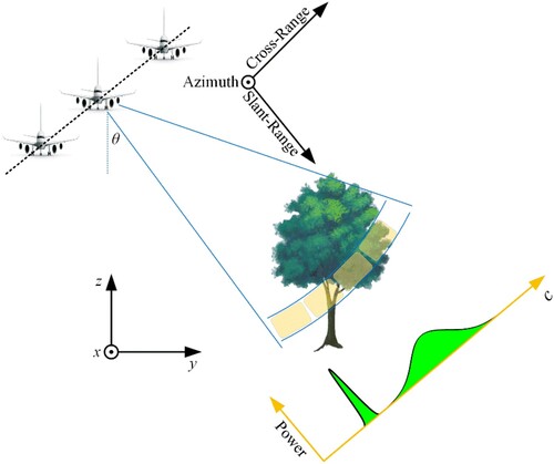
It is assumed that there are $N$ SAR images acquired at a slightly varying incidence angles along different heights over a forest area, which need to be preprocessed (such as co-registration, deramping, phase calibration (Tebaldini and Rocca 2011; Wasik et al. 2018; Lu et al. 2021), etc.) before the tomographic focusing. Figure 1 shows a geometric diagram of TomoSAR imaging over a forest area. The TomoSAR model along the vertical direction $z$ can be expressed as (Huang, Ferro-Famil, and Lardeux 2011; Li et al. 2021): (1) $u_n=\int \text{β}\left(z\right)exp\left(-j{k}_z\left(n\right)z\right)dz$(1) where $u_n$ represents the complex observation value of the $n$th image of a specified azimuth-range pixel, and $\text{β}\left(z\right)$ is the reflectivity function along the vertical direction. $k_z=4\pi b_{\mathrm{\perp }}/\lambda r\mathrm{s}\mathrm{i}\mathrm{n}\left(\theta \right)$ represents the vertical wavenumber, $b_{\mathrm{\perp }}$ is the vertical baseline, $\lambda$ represents the wavelength, $r$ denotes the slant range, and $\theta$ is the incidence angle.

Figure 1. Geometry of an airborne TomoSAR imaging system over a forest area.

To facilitate the calculation, the continuous reflectivity function can be discretely sampled in $D$ ($D>>N$) intervals along the vertical direction $z$. Multi-looking is generally required to suppress the strong coherence noise over forest areas. If it is assumed that the number of multi-looking is $L$, then the TomoSAR model becomes (Peng et al. 2021; d'Alessandro and Tebaldini 2012): (2) $\mathit{U}\left(l\right)=\mathit{A}\left(z\right)\text{β}\left(l\right)+\mathit{e}\left(l\right)l=1,\cdots ,L$(2) where $\mathit{U}$ is the $N\times 1$ observation vector, $\mathit{A}$ is the $N\times D$ steering matrix, $\text{β}$ is the $D\times 1$ unknown reflectivity vector, and $\mathit{e}$ is the $N\times 1$ noise vector.

2.2. G-Pisarenko method

The G-Pisarenko algorithm was first proposed for array signal processing (Liu et al. 2021) and was developed based on the Pisarenko method (Stoica, Li, and Tan 2008). The G-Pisarenko method is used to estimate the logarithmic values of the covariance matrix based on large-dimensional random matrix theory. According to the eigenvalues, the corresponding eigenvectors are given different weights. The estimated covariance matrix is then the weighted sum of each scattering contribution. Through this processing, the main backscattering contribution is enhanced and the secondary backscattering contribution, such as noise, is weakened. Thus, tomograms with low sidelobes can be acquired, which is helpful for the interpretation. It is worth mentioning that, although the MUSIC algorithm can also be used to solve the eigenvalues, the G-Pisarenko method does not require input parameters like the MUSIC method does, thus avoiding the problem of estimating the input parameters in a forest area.

According to the literature (Liu et al. 2021), the spectrum estimation formula obtained by the G-Pisarenko method can be expressed as: (3) ${\hat{\mathit{P}}}_{\mathrm{G}\mathrm{P}}=\mathrm{e}\mathrm{x}\mathrm{p}\left({\mathit{A}}^{\mathrm{H}}\hat{\mathit{R}}\mathit{A}\right)$(3) where $\hat{\mathit{R}}$ is the logarithmic covariance matrix (Mestre 2008; Liu et al. 2021): (4) $\hat{\mathit{R}}=\sum _{n=1}^N{I}_n{\mathit{e}}_n{\mathit{e}}_n^{\mathrm{H}}$(4) where $(\cdot {)}^{\mathrm{H}}$ represents the conjugate transpose operator. The eigenvalue factor $I_n$ is calculated by (Mestre, Rubio, and Vallet 2012): (5) $I_n=1+\left(1+\sum _{\begin{array}{c}k=1\\ k\ne n\end{array}}^N{\displaystyle \frac{{\lambda }_n}{{\lambda }_k-{\lambda }_n}-\sum _{k=1}^N{\displaystyle \frac{{\mu }_n}{{\lambda }_k-{\mu }_n}}}\right)\log {\lambda }_n+\sum _{\begin{array}{c}k=1\\ k\ne n\end{array}}^N{\displaystyle \frac{{\lambda }_k}{{\lambda }_k-{\lambda }_n}\log {\lambda }_k+\sum _{k=1}^N{\displaystyle \frac{{\mu }_k}{{\lambda }_n-{\mu }_k}\log {\mu }_k}}$(5) The constraint factor ${\mu }_1<{\mu }_2<\cdots <{\mu }_N$ can be obtained from: (6) $1={\displaystyle \frac{1}{L}\sum _{r=1}^N{\displaystyle \frac{{\lambda }_r}{{\lambda }_r-\mathit{\mu }}}}$(6)

The ${\lambda }_1<{\lambda }_2<\cdots <{\lambda }_N$ represent the eigenvalues of the complex sample covariance matrix $\mathit{R}$, and $\left\{{\mathit{e}}_n,n=1,\cdots ,N\right\}$ are the corresponding eigenvectors. The $\mathit{R}$ is processed by (del Campo, Nannini, and Reigber 2020): (7) $\mathit{R}={\displaystyle \frac{1}{L}\sum _{l=1}^L\mathit{U}\left(l\right)\mathit{U}(l{)}^{\mathrm{H}}}$(7) Finally, the workflow of the spectrum estimation method based on the G-Pisarenko algorithm can be represented as shown in Table 1.

Table 1. The G-Pisarenko tomographic spectrum estimation method.

Initialization	$\mathit{R}={\displaystyle \frac{1}{L}\sum _{l=1}^L\mathit{U}\left(l\right)\mathit{U}(l{)}^{\mathrm{H}}}$
	$\left[\mathit{e},\mathit{\lambda }\right]=\mathrm{e}\mathrm{i}\mathrm{g}\left(\mathit{R}\right)$
	$\mu \mathrm{s}.\mathrm{t}.1={\displaystyle \frac{1}{L}\sum _{r=1}^N{\displaystyle \frac{{\lambda }_r}{{\lambda }_r-\mathit{\mu }}}}$
	$\hat{\mathit{R}}=0$
For n = 1: N
	$I_n=1+\left(1+\sum _{\begin{array}{c}k=1\\ k\ne n\end{array}}^N{\displaystyle \frac{{\lambda }_n}{{\lambda }_k-{\lambda }_n}-\sum _{k=1}^N{\displaystyle \frac{{\mu }_n}{{\lambda }_k-{\mu }_n}}}\right)\log {\lambda }_n+\sum _{\begin{array}{c}k=1\\ k\ne n\end{array}}^N{\displaystyle \frac{{\lambda }_k}{{\lambda }_k-{\lambda }_n}\log {\lambda }_k+\sum _{k=1}^N{\displaystyle \frac{{\mu }_k}{{\lambda }_n-{\mu }_k}\log {\mu }_k}}$
	$\hat{\mathit{R}}=\hat{\mathit{R}}+I_n{\mathit{e}}_n{\mathit{e}}_n^{\mathrm{H}}$
end
	${\hat{\mathit{P}}}_{\mathrm{G}\mathrm{P}}=\mathrm{e}\mathrm{x}\mathrm{p}\left({\mathit{A}}^{\mathrm{H}}\hat{\mathit{R}}\mathit{A}\right)$

3. Simulation experiments

In this section, we describe how the G-Pisarenko method was applied to simulated data to verify its feasibility and effectiveness. The simulated data were obtained based on the imaging parameters of an airborne SAR system (the P-band F-SAR system) of the AfriSAR campaign over the Lope region of Gabon, as shown in Table 2. Table 3 lists the baseline information. The simulated signal was made up of ground and canopy scattering parts, which had different phase centers (0 and 30 m, respectively, i.e. $\mathrm{\Delta }H=30\mathrm{m}$). The canopy scattering signal had a larger angular spread than the ground scattering signal.

Table 2. Parameters of the P-band F-SAR airborne SAR system.

Parameter	Value
Platform height	6096 m
Wavelength	0.6890 m
Incidence angle	20°−50°
Range resolution	3.84 m
Azimuth resolution	2 m
Polarization mode	HH + HV + VV

Table 3. Baseline information of the used datasets from the Lope region.

Identifier	Date of acquisition	Baseline (m)
FL06-PS02	10-Feb-2016	0
FL06-PS03		10
FL06-PS05		40
FL06-PS07		80
FL06-PS08		−20
FL06-PS11		−80

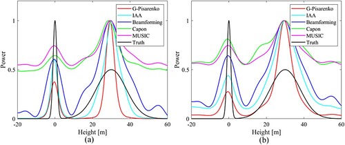
Figure 2 shows the inversion capability of five different methods in the case of a high and low signal-to-noise ratio (SNR) with a large height difference ($\mathrm{\Delta }H=30\mathrm{m}$). As can be seen from Figure 2(a), in the case of high SNR (20 dB), the ground and canopy scattering phase centers can be successfully found by all five methods, but a serious sidelobe effect is apparent for the Beamforming, Capon, and MUSIC methods. The results obtained by the IAA and G-Pisarenko methods show only a slight sidelobe effect. Moreover, with the reduction of the SNR (as shown in Figure 2(b)), all five methods are affected by the noise, and the sidelobe effect becomes more serious; however, the G-Pisarenko method is the least affected. Therefore, the G-Pisarenko method is the most robust among these methods.

Figure 2. Comparison of the different methods for $\mathrm{\Delta }H=30\mathrm{m}$ with different SNRs: (a) SNR = 20 dB; (b) SNR = 5 dB.

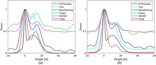
As shown in Figure 3, when the ground and canopy scattering phase centers are close to each other (0 and 10 m, respectively, i.e. $\mathrm{\Delta }H=10\mathrm{m}$), all five methods can find the ground scattering phase center, but there is bias between the estimation of the canopy phase center height and the truth. As in the case of $\mathrm{\Delta }H=30\mathrm{m}$, the G-Pisarenko method inhibits the noise signal in the tomogram and reduces the sidelobe effect. Moreover, the inversion performance of the G-Pisarenko method is superior to that of the other methods under the low SNR case.

Figure 3. Comparison of the different methods for $\mathrm{\Delta }H=10\mathrm{m}$ with different SNRs: (a) SNR = 20 dB; (b) SNR = 5 dB.

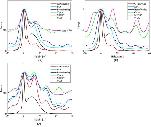
In addition, we also tested the performance of the proposed method under different numbers of looks and images, as shown in Figure 4. It is clear that all five methods perform better in the case of a large number of looks and images. This is because reducing the number of multi-looks $L$ can enhance the influence of the observation noise (comparing subfigures (a) and (b)), and reducing the number of images $N$ brings a more serious sidelobe effect (comparing subfigures (a) and (c)). In both cases, the G-Pisarenko method outperforms the other methods.

Figure 4. Comparison of different numbers of multi-looks ($L$) and images ($N$): (a) $L=100$, $N=6$; (b) $L=20$, $N=6$; (c) $L=100$, $N=4$.

As for the reflectivity estimation, the Beamforming method can perform better than the other four methods. This is because Beamforming can obtain the true reflectivity directly, while the other methods are not radiometrically correct. If the forest structure reconstruction was to be further analyzed, it would be necessary for these four methods to calculate the true reflectivity based on a least square equation (Huang, Ferro-Famil, and Reigber 2011).

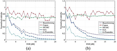
In addition, we also calculated the normalized sidelobe levels of the five methods for SNR levels ranging from −5 dB to 20 dB (as shown in Figure 5). The normalized sidelobe level is represented as the normalized area between the backscattering power curve and the x-axis on the non-main lobe interval. As can be seen in Figure 5, the sidelobe level of the G-Pisarenko method is less than half that of the other methods when the noise is strong (i.e. SNR = −5 dB). With the increase of the SNR, the G-Pisarenko method maintains the obvious advantage of the low sidelobe level, and no sidelobes are apparent at the range of [15, 20] dB. The above analysis demonstrates that the G-Pisarenko method greatly reduces the sidelobe effect in TomoSAR.

Figure 5. Normalized sidelobe levels for the SNR in different $\mathrm{\Delta }H$ values: (a) $\mathrm{\Delta }H=10$ m; (b) $\mathrm{\Delta }H=30$ m.

It can be seen from the above analysis that, compared with the other four methods, the G-Pisarenko method shows better robustness to noise, which is conducive to image interpretation and information extraction.

4. Real data experiments and results

4.1. Study area and datasets

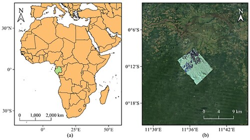
The study area is located in the Lope region of Gabon, north-east Africa (see Figure 6), and is 250 km away from the Libreville capital airport. The Lope region is characterized by a savannah and (dense) tropical forest mosaic. The area is a predominantly hilly tropical forest region, with topographic relief ranging from 163 to 583 m. In addition, the local slope of some areas can exceed 20°, and the maximum forest height is more than 70 m.

Figure 6. (a) Gabon, Africa (green polygon) and (b) the Pauli RGB image of the study area.

In order to further verify the advantages of the G-Pisarenko method, 3D tomographic imaging was carried out with six P-band fully polarized images obtained as part of the airborne AfriSAR campaign (European Space Agency 2016). AfriSAR was an ESA-funded airborne P-band SAR campaign conducted over the tropical forest of Gabon that was carried out by ONERA (July 2015) and DLR (February 2016) in support of the development of the geophysical algorithms for the future BIOMASS mission (Hajnsek et al. 2016). The campaign design addressed the geophysical BIOMASS products (forest above-ground biomass, forest upper canopy height, and disturbances) by implementing PolSAR (SAR polarimetry), PolInSAR (polarimetric SAR interferometry), and TomoSAR techniques with P-band measurements over the selected test sites (Fatoyinbo et al. 2021). The used datasets were collected over the Lope region of Gabon, Africa, and LiDAR digital terrain model (DTM) and canopy height model (CHM) were also acquired for the validation.

4.2. Profile analysis

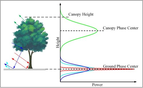
As shown in Figure 7, according to the existing forest SAR imaging principle, four kinds of scattering mechanisms exist over forest areas: surface scattering from the ground (the cyan curve), double-bounce scattering from tree trunks to the ground (the red curve), double-bounce scattering from the canopy to the ground (the blue curve), and volume scattering from the canopy (the green curve). The first three kinds of phase centers are fixed on the ground, while the scattering phase center of the last mechanism is in the middle of the canopy, rather than the top. Therefore, the location of the lower peak from the tomogram’s main lobe is usually the underlying topography, and the upper peak’s position is the forest canopy phase center height.

Figure 7. The distribution of the forest backscattering mechanism power with elevation.

In order to demonstrate the inversion performance of the proposed method, a profile (the red solid line in Figure 8) from the near ground range to far ground range in the study area was selected for 3D tomographic imaging. As shown in Figure 9, the underlying topography and canopy height are more or less estimated by all five methods in the three polarizations. However, the G-Pisarenko method shows a better performance than Beamforming, Capon, MUSIC, and IAA in terms of noise suppression. Moreover, an obvious sidelobe effect is apparent in the results of the first four methods (Beamforming, Capon, MUSIC, and IAA), while the estimation of the G-Pisarenko method is only slightly affected by sidelobes. These sidelobes would likely affect the detection of the ground and canopy phase centers. It can be seen from the results estimated by the G-Pisarenko method (the last row in Figure 9) that most of the sidelobe information, except for the main lobe, is weakened, which is beneficial when setting a fixed peak threshold to search for the height of the ground and canopy phase centers. For the other four methods, it is difficult to specify a fixed peak threshold globally to accomplish the above operation. This indicates that the G-Pisarenko method has obvious advantages over the other methods.

Figure 8. Selected profile (red solid line) on the Pauli RGB image.

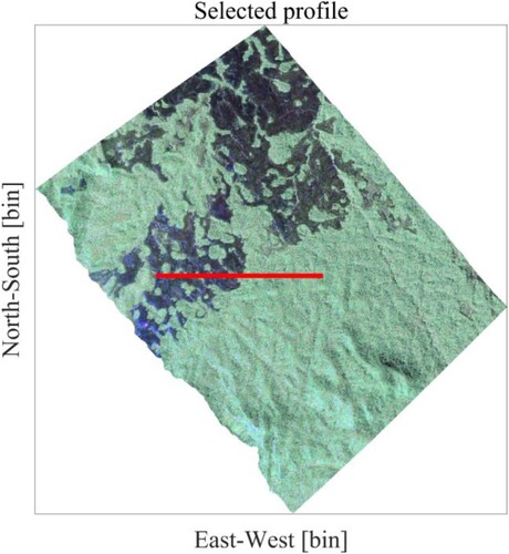
Figure 9. Tomograms of the HH (left column), HV (middle column), and VV (right column) channels on the selected range profile: (a), (f), and (k) Beamforming; (b), (g), and (l) Capon; (c), (h), and (m) MUSIC; (d), (i), and (n) IAA; (e), (j), and (o) G-Pisarenko. The black solid lines and white dotted lines denote the LiDAR DTM and CHM, respectively.

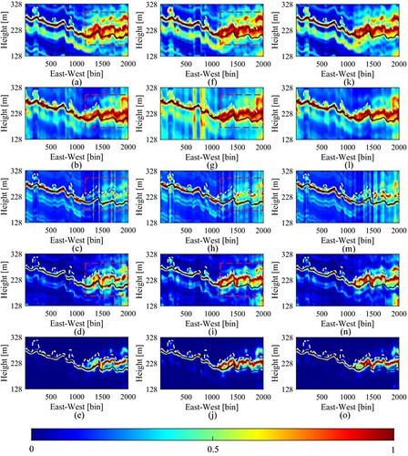
Furthermore, the underlying topography of the selected profile was also estimated, as shown in Figure 10(a). It is clear that, in the near ground range, the underlying topography obtained by Beamforming, Capon, and MUSIC is roughly similarly to the LiDAR measurements, with some deviations. The results of the IAA and G-Pisarenko methods are also in good agreement with the LiDAR measurements. In the far ground range, except for the G-Pisarenko method, the other four methods show large deviations in certain places, and they fail to separate the ground and canopy scattering phase centers. The main reason for this is the sidelobe effect (the red dotted rectangles in the first column of Figure 9) in the far ground range.

Figure 10. The estimated results obtained by the TomoSAR methods for the selected profile: (a) underlying topography, (b) forest canopy.

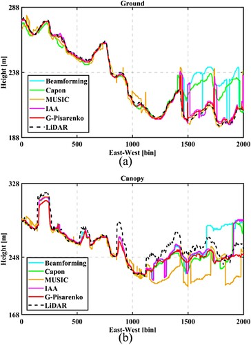
In addition, the canopy scattering phase center height for the selected profile was also estimated, as shown in Figure 10(b). In the near ground range, all of these estimators can detect the canopy phase center height. However, the MUSIC method shows some misestimation in several regions. In the far ground range, the Beamforming, Capon, MUSIC, and IAA methods are more or less affected by the sidelobe effect (the red dotted rectangles in the second column of Figure 9), resulting in wrong detection of the canopy phase center height. In contrast, the estimation of the G-Pisarenko method is similar to the LiDAR CHM. In summary, the G-Pisarenko method achieves the best performance among these methods in underlying topography and forest height estimation.

Furthermore, the computation times of the five methods were analyzed quantitatively, as shown in Table 4. For the selected range profile, the running time of the G-Pisarenko method is more than three times that of the other methods for the same computer (a Linux server with an AMD Ryzen 9 5900X 12-core processor) because it needs more times to solve a multivariate equation (i.e. Equation (6)).

Table 4. Running times of the different methods for estimating the selected profile.

Method	Time [s]
Beamforming	70
Capon	84
MUSIC	69
IAA	87
G-Pisarenko	238

5. Discussion

5.1 Underlying topography estimation

According to the existing research (Tebaldini et al. 2019; Aghababaee et al. 2020; Yu and Zhang 2021), the backscattering reflectivity of the HH polarization channel mainly comes from the ground, the backscattering power of the HV polarization channel is mainly concentrated on the canopy volume scattering, and the backscattering contribution of the VV polarization channel is between the HH and HV polarization channels. This is also confirmed by Figure 9. Thus, tomograms of the HH channel and HV channel are generally used in estimating ground height and canopy height.

The DTMs of the whole study area were estimated by the five methods, as shown in Figure 11. These results are, on the whole, close to the LiDAR DTM. Moreover, further analysis was conducted to compare the performance of the five methods. Figure 12 shows a comparison between the underlying topography obtained by the different TomoSAR methods and the LiDAR DTM. The range of ground height values in the TomoSAR results and LiDAR is consistent. We also calculated the $R^2$ values for the Beamforming, Capon, MUSIC, IAA, and G-Pisarenko methods, which are 0.853, 0.873, 0.882, 0.900, and 0.965, respectively. This indicates that the estimation accuracy of the G-Pisarenko method is the best. In addition, the mean error and the root-mean-square error (RMSE) with respect to LiDAR were also calculated, as shown in Table 5. The RMSE of the proposed method is 7.26 m, while the RMSEs for the Beamforming, Capon, MUSIC, and IAA methods are 9.15, 8.72, 8.28, and 8.03 m, respectively. Furthermore, the improvement ratio of the G-Pisarenko method with respect to Beamforming, Capon, MUSIC, and IAA is 27%, 22%, 18%, and 10%, respectively. This implies that the G-Pisarenko method shows a considerable improvement over the other four methods. The above analysis demonstrates that the G-Pisarenko method shows a superior performance in estimating the underlying topography.

Figure 11. Estimated DTMs: (a) Beamforming, (b) Capon, (c) MUSIC, (d) IAA, (e) G-Pisarenko; referenced DTM: (f) LiDAR.

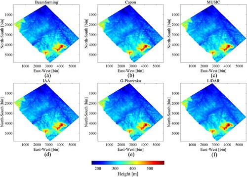
Figure 12. 2D joint distribution between the LiDAR DTM measurements and the estimations of the five methods for the selected range profile: (a) Beamforming, (b) Capon, (c) MUSIC, (d) IAA, (e) G-Pisarenko.

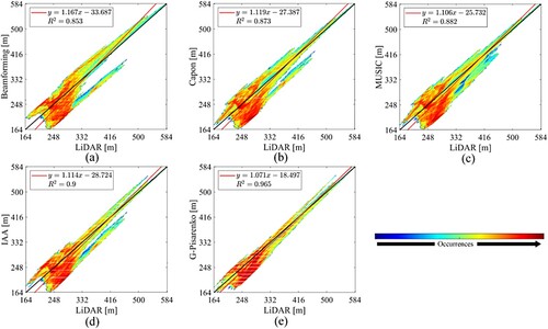
Table 5. The mean error and RMSE of the different methods for the underlying topography of the whole study area.

Method	Mean error (m)	RMSE (m)
Beamforming	4.95	9.15
Capon	4.49	8.72
MUSIC	3.96	8.28
IAA	3.67	8.03
G-Pisarenko	2.81	7.26

5.2. Forest height estimation

As stated in Section 5.1, tomograms in HV polarization can indicate the canopy backscattering phase center height. However, it is usually necessary to evaluate the power loss with respect to the phase center to calculate the canopy top height. Details of this process can be found in the literature (Tebaldini 2009; Ho Tong Minh et al. 2016; Tebaldini and Rocca 2011). We calculated the RMSE between the LiDAR CHM and the estimated heights under different power loss values. As shown in Figure 13, the RMSE of the forest height estimated by the G-Pisarenko method relative to the LiDAR CHM reaches the minimum when the power loss is −4 dB, and the other methods show the smallest difference between the estimations and the LiDAR CHM in the case of a power loss of −3 dB. These two values were therefore used to estimate the canopy height. After this, the forest height can be obtained through subtracting the underlying topography from the canopy top height. The forest heights obtained by the five methods are shown in Figure 14. It is clear that the estimation of the G-Pisarenko method is the closest to the LiDAR CHM. In order to quantitatively analyze the performance of these five methods in forest height inversion, the mean errors and RMSEs of the five methods with respect to the LiDAR CHM were also obtained (see Table 6). The inversion accuracy of the G-Pisarenko method is the best, with an RMSE of 2.58 m. When compared with the Beamforming, Capon, MUSIC, and IAA methods, the G-Pisarenko method improves the estimation accuracy by 39%, 33%, 27%, and 19%, respectively.

Figure 13. RMSE between the LiDAR CHM and TomoSAR CHM with different power loss values.

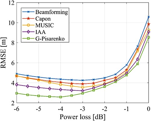
Figure 14. Estimated CHM: (a) Beamforming, (b) Capon, (c) MUSIC, (d) IAA, (e) G-Pisarenko; referenced CHM: (f) LiDAR.

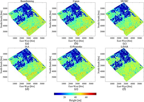
Table 6. The mean error and RMSE of the different methods for the forest heights of the whole study area.

Method	Mean error (m)	RMSE (m)
Beamforming	−0.38	4.25
Capon	−0.35	3.89
MUSIC	−0.18	3.55
IAA	−0.25	3.21
G-Pisarenko	−0.23	2.58

We show the 2D joint distribution histogram between the estimated results and the LiDAR CHM in Figure 15. As can be clearly seen from Figure 15, the fitting performance between the estimation of the proposed method and the LiDAR CHM is the best, with the $R^2$ value reaching 0.899, which is significantly better than the other four methods. In order to further evaluate the forest height estimation accuracy, the relative error of the forest height was calculated according to $\left|h_{\mathrm{t}\mathrm{o}\mathrm{m}\mathrm{o}}-h_{\mathrm{l}\mathrm{i}\mathrm{d}\mathrm{a}\mathrm{r}}\right|/h_{\mathrm{l}\mathrm{i}\mathrm{d}\mathrm{a}\mathrm{r}}$. 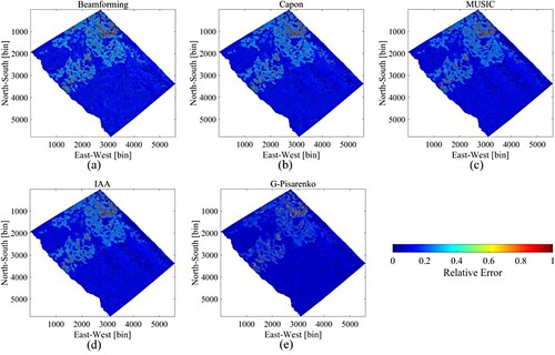$h_{\mathrm{t}\mathrm{o}\mathrm{m}\mathrm{o}}$ is the forest height estimated by the TomoSAR method, and $h_{\mathrm{l}\mathrm{i}\mathrm{d}\mathrm{a}\mathrm{r}}$ is the LiDAR measurement. Figure 16 shows the relative error between the LiDAR CHM and the estimated forest height. It is clear that the inversion error of the five methods in the area of low vegetation is higher than that in the area of high vegetation. Moreover, the relative error of the G-Pisarenko method for most areas is less than 30%, and the average relative error is 12.04%. All five methods show some overestimation or underestimation, and this phenomenon mainly appears in the low vegetation area (as shown in Figure 16), which is consistent with the exist research (Yang et al. 2019). Nevertheless, the proposed method can minimize the sidelobe effect caused by noise, so as to achieve better inversion results.

Figure 15. 2D joint distribution between the LiDAR CHM measurements and the estimations of the five methods for the selected range profile: (a) Beamforming, (b) Capon, (c) MUSIC, (d) IAA, (e) G-Pisarenko.

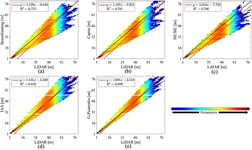
Figure 16. The estimated CHM relative error: (a) Beamforming w.r.t LiDAR, (b) Capon w.r.t LiDAR, (c) MUSIC w.r.t LiDAR, (d) IAA w.r.t LiDAR, (e) G-Pisarenko w.r.t LiDAR.

6. Conclusions

In this paper, a nonparametric spectrum estimation method has been introduced for the tomographic imaging of forest areas: the G-Pisarenko method. This method uses a logarithmic operation to estimate the covariance matrix, and extracts the scattering characteristics of the target objects, which is helpful for obtaining the underlying topography and forest height.

We carried out validation experiments using both simulated data and real data. In the simulation experiments, the simulated signal was used to explore the performance of the proposed method under different SNRs and different ground-canopy height differences. The G-Pisarenko method not only discriminated the ground and canopy phase centers, but it also maintained a lower sidelobe level (compared to Beamforming, Capon, MUSIC, and IAA) under different ground-canopy height differences. Furthermore, with the increase of the SNR, it was found that the normalized sidelobe level of the G-Pisarenko method converges much faster. In the real data experiments, both the underlying topography and forest height were estimated using six P-band fully polarimetric airborne images from the Lope region of Gabon, Africa. The results showed that the G-Pisarenko method can effectively suppress the noise, and there is almost no sidelobe effect to affect the interpretation of the tomograms. Moreover, the estimation accuracy of the G-Pisarenko method was higher than that of the other four methods, by more than 20%. All the results verified that the G-Pisarenko method is a good candidate for underlying topography and forest height estimation.

However, the G-Pisarenko method requires more computation time to compute the tomograms, because it needs to solve a multivariate equation (i.e. Equation (6)). In our future work, we will continue to improve this method and increase the inversion accuracy in forest structure reconstruction.

Acknowledgements

The authors would like to thank the DLR, ESA, and the AfriSAR team for providing the AfriSAR datasets. Authors conribution: Youjun Wang: Conceptualization, Methodology, Formal analysis, Software, Visualization, and Writing – original draft preparation. Xing Peng: Methodology, Validation, Formal analysis, Writing – review and editing, and Supervision and Funding acquisition. Qinghua Xie: Investigation, Funding acquisition and Writing – review and editing. Xinwu Li: Formal analysis, Investigation, and Funding acquisition. Xiaomin Luo: Writing – review and editing. Yanan Du: Investigation and Writing – review and editing. Bing Zhang: Investigation and Writing – review and editing.

Disclosure statement

No potential conflict of interest was reported by the author(s).

Additional information

Funding

This work was supported in part by the National Natural Science Foundation of China [grant number 42101400], [grant number 42171387]; and in part by the Strategic Priority Research Program of the Chinese Academy of Sciences [grant number XDA19070202].

References

- Aghababaee, H., G. Ferraioli, L. Ferro-Famil, Y. Huang, M. M. d'Alessandro, V. Pascazio, G. Schirinzi, and S. Tebaldini. 2020. “Forest SAR Tomography: Principles and Applications.” IEEE Geoscience and Remote Sensing Magazine 8 (2): 30–45. doi:10.1109/MGRS.2019.2963093.
- Budillon, A., A. Evangelista, and G. Schirinzi. 2009. “SAR Tomography from Sparse Samples.” 2009 IEEE International Geoscience and Remote Sensing Symposium, Cape Town, South Africa.
- Cazcarra-Bes, V., M. Pardini, and K. Papathanassiou. 2020. “Definition of Tomographic SAR Configurations for Forest Structure Applications at L-Band.” IEEE Geoscience and Remote Sensing Letters, doi:10.1109/LGRS.2020.3027439.
- Cazcarra-Bes, V., M. Pardini, M. Tello, and K. P. Papathanassiou. 2019. “Comparison of Tomographic SAR Reflectivity Reconstruction Algorithms for Forest Applications at L-Band.” IEEE Transactions on Geoscience and Remote Sensing 58 (1): 147–164. doi:10.1109/TGRS.2019.2934347.
- d'Alessandro, M. M., and S. Tebaldini. 2012. “Phenomenology of P-Band Scattering from a Tropical Forest Through Three-Dimensional SAR Tomography.” IEEE Geoscience and Remote Sensing Letters 9 (3): 442–446. doi:10.1109/LGRS.2011.2170658.
- del Campo, G. M., M. Nannini, and A. Reigber. 2020. “Statistical Regularization for Enhanced TomoSAR Imaging.” IEEE Journal of Selected Topics in Applied Earth Observations and Remote Sensing 13: 1567–1589. doi:10.1109/JSTARS.2020.2970595.
- European Space Agency. 2016. “AfriSAR 2016: Technical Assistance for the Development of Airborne SAR and Geophysical Measurements During the AfriSAR Experiment - Final Report.” https://earth.esa.int/eogateway/campaigns/afrisar-2016?text = afrisar.
- Fatoyinbo, T., J. Armston, M. Simard, S. Saatchi, M. Denbina, M. Lavalle, M. Hofton, H. Tang, S. Marselis, and N. Pinto. 2021. “The NASA AfriSAR Campaign: Airborne SAR and Lidar Measurements of Tropical Forest Structure and Biomass in Support of Current and Future Space Missions.” Remote Sensing of Environment 264: 112533. doi:10.1016/j.rse.2021.112533.
- Ferro-Famil, L., Y. Huang, and A. Reigber. 2012. “High-resolution SAR Tomography Using Full Rank Polarimetric Spectral Estimators.” IEEE International Geoscience and Remote Sensing Symposium, 5194–5197. doi:10.1109/IGARSS.2012.6352439.
- Hajnsek, I., M. Pardini, R. Horn, R. Scheiber, K. Papathanassiou, P. D. Fernandez, R. Baque, X. Dupuis, and T. Casal. 2016. “Sar Imaging of Tropical African Forests with P-Band Multibaseline Acquisitions: Results from the Afrisar Campaign.” 2016 IEEE International Geoscience and Remote Sensing Symposium (IGARSS), Beijing, China.
- Homer, J., I. Longstaff, and G. Callaghan. 1996. “High Resolution 3-D SAR via Multi-Baseline Interferometry.” 1996 IEEE International Geoscience and Remote Sensing Symposium (IGARSS), Lincoln, NE, USA.
- Ho Tong Minh, D., T. Le Toan, F. Rocca, S. Tebaldini, L. Villard, M. Réjou-Méchain, O. L. Phillips, T. R. Feldpausch, P. Dubois-Fernandez, and K. Scipal. 2016. “SAR Tomography for the Retrieval of Forest Biomass and Height: Cross-Validation at Two Tropical Forest Sites in French Guiana.” Remote Sensing of Environment 175: 138–147. doi:10.1016/j.rse.2015.12.037.
- Huang, Y., L. Ferro-Famil, and C. Lardeux. 2011. “Polarimetric SAR Tomography of Tropical Forests at P-Band.” 2011 IEEE International Geoscience and Remote Sensing Symposium (IGARSS), Vancouver, British Columbia, Canada.
- Huang, Y., L. Ferro-Famil, and A. Reigber. 2011. “Under-foliage Object Imaging Using SAR Tomography and Polarimetric Spectral Estimators.” IEEE Transactions on Geoscience and Remote Sensing 50 (6): 2213–2225. doi:10.1109/TGRS.2011.2171494.
- Huang, Y., J. Levy-Vehel, L. Ferro-Famil, and A. Reigber. 2017. “Three-dimensional Imaging of Objects Concealed Below a Forest Canopy Using SAR Tomography at L-Band and Wavelet-Based Sparse Estimation.” IEEE Geoscience and Remote Sensing Letters 14 (9): 1454–1458. doi:10.1109/LGRS.2017.2709839.
- Huang, Y., Q. Zhang, and L. Ferro-Famil. 2021. “Forest Height Estimation Using a Single-Pass Airborne L-Band Polarimetric and Interferometric SAR System and Tomographic Techniques.” Remote Sensing 13 (3): 487. doi:10.3390/rs13030487.
- Li, X., L. Liang, H. Guo, and Y. Huang. 2016. “Compressive Sensing for Multibaseline Polarimetric SAR Tomography of Forested Areas.” IEEE Transactions on Geoscience and Remote Sensing 54 (1): 153–166. doi:10.1109/TGRS.2015.2451992.
- Li, Z., P. Zhang, H. Qiao, C. Zhao, J. Zhou, and L. Huang. 2021. “Advances in Information Extraction of Surface Parameters Using Tomographic SAR.” Journal of Radars 10 (1): 116–130. doi:10.12000/JR20095.
- Liu, Y., J. Zhao, Q. Zhu, and Y. Wang. 2021. “An Improved Method for Parametric Spatial Spectrum Estimation in Internet of Things.” Wireless Communications and Mobile Computing 2021. doi:10.1155/2021/9976751.
- Lombardini, F., and A. Reigber. 2003. “Adaptive Spectral Estimation for Multibaseline SAR Tomography with Airborne L-Band Data.” 2003 IEEE International Geoscience and Remote Sensing Symposium (IGARSS), Toulouse, France.
- Lu, H., H. Zhang, H. Fan, D. Liu, J. Wang, X. Wan, L. Zhao, Y. Deng, F. Zhao, and R. Wang. 2021. “Forest Height Retrieval Using P-Band Airborne Multi-Baseline SAR Data: A Novel Phase Compensation Method.” ISPRS Journal of Photogrammetry and Remote Sensing 175: 99–118. doi:10.1016/j.isprsjprs.2021.02.022.
- Mestre, X. 2008. “Improved Estimation of Eigenvalues and Eigenvectors of Covariance Matrices Using Their Sample Estimates.” IEEE Transactions on Information Theory 54 (11): 5113–5129. doi:10.1109/TIT.2008.929938.
- Mestre, X., F. Rubio, and P. Vallet. 2012. “Improved Estimation of the Logarithm of the Covariance Matrix.” 2012 IEEE 7th Sensor Array and Multichannel Signal Processing Workshop (SAM), Hoboken, NJ, USA.
- Mukherjee, S., P. K. Joshi, S. Mukherjee, A. Ghosh, R. Garg, and A. Mukhopadhyay. 2013. “Evaluation of Vertical Accuracy of Open Source Digital Elevation Model (DEM).” International Journal of Applied Earth Observation and Geoinformation 21: 205–217. doi:10.1016/j.jag.2012.09.004.
- Nannini, M., R. Scheiber, and A. Moreira. 2009. “Estimation of the Minimum Number of Tracks for SAR Tomography.” IEEE Transactions on Geoscience and Remote Sensing 47 (2): 531–543. doi:10.1109/TGRS.2008.2007846.
- Pardini, M., V. Cazcarra-Bes, and K. P. Papathanassiou. 2021. “TomoSAR Mapping of 3D Forest Structure: Contributions of L-Band Configurations.” Remote Sensing 13 (12): 2255. doi:10.3390/rs13122255.
- Peng, X., X. Li, C. Wang, H. Fu, and Y. Du. 2018. “A Maximum Likelihood Based Nonparametric Iterative Adaptive Method of Synthetic Aperture Radar Tomography and its Application for Estimating Underlying Topography and Forest Height.” Sensors 18 (8): 2459. doi:10.3390/s18082459.
- Peng, X., Y. Wang, S. Long, X. Pan, Q. Xie, Y. Du, H. Fu, J. Zhu, and X. Li. 2021. “Underlying Topography Inversion Using TomoSAR Based on Non-Local Means for an L-Band Airborne Dataset.” Remote Sensing 13 (15): 2926. doi:10.3390/rs13152926.
- Reigber, A., and A. Moreira. 2000. “First Demonstration of Airborne SAR Tomography Using Multibaseline L-Band Data.” IEEE Transactions on Geoscience and Remote Sensing 38 (5): 2142–2152. doi:10.1109/36.868873.
- Stoica, P., P. Babu, and J. Li. 2010. “SPICE: A Sparse Covariance-Based Estimation Method for Array Processing.” IEEE Transactions on Signal Processing 59 (2): 629–638. doi:10.1109/TSP.2010.2090525.
- Stoica, P., J. Li, and X. Tan. 2008. “On Spatial Power Spectrum and Signal Estimation Using the Pisarenko Framework.” IEEE Transactions on Signal Processing 56 (10): 5109–5119. doi:10.1109/TSP.2008.928935.
- Tebaldini, S. 2009. “Algebraic Synthesis of Forest Scenarios from Multibaseline PolInSAR Data.” IEEE Transactions on Geoscience and Remote Sensing 47 (12): 4132–4142. doi:10.1109/TGRS.2009.2023785.
- Tebaldini, S., D. H. T. Minh, M. M. d’Alessandro, L. Villard, T. Le Toan, and J. Chave. 2019. “The Status of Technologies to Measure Forest Biomass and Structural Properties: State of the Art in SAR Tomography of Tropical Forests.” Surveys in Geophysics 40 (4): 779–801. doi:10.1007/s10712-019-09539-7.
- Tebaldini, S., and F. Rocca. 2011. “Multibaseline Polarimetric SAR Tomography of a Boreal Forest at P-and L-Bands.” IEEE Transactions on Geoscience and Remote Sensing 50 (1): 232–246. doi:10.1109/TGRS.2011.2159614.
- Wasik, V., P. C. Dubois-Fernandez, C. Taillandier, and S. S. Saatchi. 2018. “The AfriSAR Campaign: Tomographic Analysis with Phase-Screen Correction for P-Band Acquisitions.” IEEE Journal of Selected Topics in Applied Earth Observations and Remote Sensing 11 (10): 3492–3504. doi:10.1109/JSTARS.2018.2831441.
- Yang, X., S. Tebaldini, M. M. d’Alessandro, and M. Liao. 2019. “Tropical Forest Height Retrieval Based on P-Band Multibaseline SAR Data.” IEEE Geoscience and Remote Sensing Letters 17 (3): 451–455. doi:10.1109/LGRS.2019.2923252.
- Yardibi, T., J. Li, P. Stoica, M. Xue, and A. B. Baggeroer. 2010. “Source Localization and Sensing: A Nonparametric Iterative Adaptive Approach Based on Weighted Least Squares.” IEEE Transactions on Aerospace and Electronic Systems 46 (1): 425–443. doi:10.1109/TAES.2010.5417172.
- Yu, H., and Z. Zhang. 2021. “The Performance of Relative Height Metrics for Estimation of Forest Above-Ground Biomass Using L-and X-Bands TomoSAR Data.” IEEE Journal of Selected Topics in Applied Earth Observations and Remote Sensing 14: 1857–1871. doi:10.1109/JSTARS.2021.3051081.