Extraction of ocean tidal information based on global equal-area grid and satellite altimeter data

ABSTRACT

Harmonic analysis of satellite altimetry data based on a global regular grid is affected by the grid spatial tessellation and placement of the grids. With the increase of latitude, the traditional lat/lon grid deforms greatly, resulting in uneven distribution of satellite altimeter data with latitude, which affects the extraction of tidal information. Alternatively, Hexagonal grids have been proved to be advantageous due to their isotropic, uniform neighbourhood, equal-area and more. Considering the merits above, the purpose of this paper is to use the global equal-area hexagonal grid to conduct a harmonic analysis of satellite altimeter data. First, the Icosahedron Snyder Equal Area projection method is used to construct a global equal-area hexagonal grid, Then the time series data of 19.8 years of Jason series satellite altimeter data are obtained. Finally, the harmonic constants of eight constituents (the M₂, S₂, N₂, K₂, K₁, O₁, P₁, Q₁) are extracted by harmonic analysis. By analysing the results, we conclude that the harmonic constants extracted from the global equal-area hexagonal grid have considerable accuracy and are consistent with the tidal characteristics of the eight components. Meanwhile, the accuracy of harmonic constants extracted from equal-area hexagonal grids is better than that of lat/lon grids.

KEYWORDS:

• Equal-area
• hexagonal grids
• satellite altimeter data
• harmonic analysis

1. Introduction

Ocean tide is a common natural phenomenon, which is the periodic fluctuation of sea water caused by the tidal forces of the sun and moon. The tidal signal is crucial in a wide range of dynamic ocean systems ranging from the turbulent mixing of the ocean (Egbert & Ray, 2000; Mackinnon et al., 2017; Munk & Wunsch, 1998) to the prediction of coastal sea levels (Bernier & Thompson, 2007; Tang, Sanderson, Holland, & Grimshaw, 1996). Therefore, the study of ocean tide directly affects the study of waves, Strom surges, circulation and other ocean phenomena.

At present, research methods for ocean tidal information extraction include the empirical tidal model (Cheng & Andersen, 2011; Ray, 1999), the hydrodynamic model (Arbic, Mitrovica, Macayeal, & Milne, 2008; Green & Nycander, 2013; Hill, Griffiths, Peltier, Horton, & Törnqvist, 2011) and the assimilation model (Lyard, Lefevre, Letellier, & Francis, 2006; Schwiderski, 1979; Taguchi, Stammer, & Zahel, 2014). In these three ways, the empirical tidal model is completely dependent on the actual observation data. Although its physical signification is not as clear as that of the dynamic model, the modelling process of the empirical tidal model is simple, direct, practical and efficient, and will not be affected by the uncertainties of parameters such as the bottom friction coefficient in the dynamic equation. Therefore, the empirical tidal model has always been an important method in the extraction of ocean tidal parameters.

The empirical tidal modelling method is to calculate the harmonic constants of tides directly from satellite altimeter data using the appropriate tidal analysis method. There are three kinds of analysis methods in common use at present, including along track analysis, crossover points analysis and block analysis.

Along track analysis and crossover points analysis are both based on single-point altimeter analysis. Along track analysis is to extract tidal information point by point along the satellite track(Foreman, Cherniawsky, & Ballantyne, 2009; Ray, 1999; Yanagi, Morimoto, & Ichikawa, 1997). Due to the influence of external forces on the satellite in different operating periods, the data points differ every cycle. Scholars need to linearly interpolated observed data at the fixed points along the sub-satellite track(Van Gysen, Coleman, Morrow, Hirsch, & Rizos, 1992). According to the sampling rule of satellite altimeter, altimeter data can be obtained every second (5–6 km). Hence, the altimeter data is highly utilized by analysis along the track. This is very efficient for the regional ocean, but for the large-scale ocean, it not only requires complex data adjustment calculation but also causes great data redundancy. Crossover points analysis is to extract tidal information by the crossing points of ascending and descending tracks (Bao, Chao, & Li, 2000; Egbert & Ray, 2000; Fang, 2016). It is very rare to have observed values at the crossing points, and it is often necessary to select several measured data near the possible crossing points and use polynomial fitting to determine the position of the crossing points (Tai, 1988). Therefore, crossover point analysis not only involves a lot of adjustment calculation but also discards a large number of altimeter data at non-intersection points.

To make full and reasonable use of satellite altimeter data, block analysis is a better method. In this method, all the altimeter data in the grid cells are taken as the observation data in the centre of the grid to obtain the tidal information with average significance. This method of average is more suitable for large areas of open ocean (Bao, Chao, Li, & Deng 1999). At present, the lat/lon grids are used in the method of regional block analysis. However, as the latitude increases, the geometry and area of the grid will change. This method not only results in the difference in the quantity distribution of satellite altimeter data in different grids but also the probability of satellite altimeter data being dropped into the grids is not equal. Therefore, the lat/lon grids will adversely affect ocean tidal information extraction.

The fundamental reason for this problem is that the lat/lon grid is non-equal area grid, which cannot achieve uniform sampling on a global scale. The essence of the regional block analysis method is to uniformly sample and interpolate long-term satellite altimeter data, Kmoch, Vasilyev, Virro, and Uuemaa (2022) have also demonstrated that equal-area grids are more suitable for global statistics. Therefore, using global equal-area grids for satellite altimeter data processing is expected to improve the accuracy of global ocean tidal information extraction.

The remaining sections of this paper are arranged as follows. In the second section, we analyse the research progress of global ocean tide information extraction based on satellite altimeter data and global equal-area grids. Based on this part, in the third section, we introduce the basic ideas of extracting ocean tidal information based on harmonic analysis. In the fourth section, the global equal-area hexagonal discrete grid is constructed based on Snyder Equal-area Projection. Then, the method for extracting tidal information based on the global equal-area hexagonal grid is developed. In the fifth section, Harmonic constant information is extracted from the global ocean through 19.8 years of long-period satellite altimeter data. Finally, the sixth and seventh sections discuss and summarize the findings of this study.

2. Related works

2.1. Global ocean tidal information extraction based on satellite altimeter data

Under the current international development background of ocean tidal information extraction, it is the simplest and most effective way to extract ocean harmonic constants directly from satellite altimetry data (Li, 2013). Therefore, it’s necessary to summarize the research progress of global ocean tidal information extraction.

The principle of extracting ocean tidal information based on satellite altimeter data is to use the time series data obtained by the satellite altimeter to tide analysis and to solve the harmonic constants which characterize the law of tidal variation. However, the sampling interval of altimeter satellites performing precise repetitive trajectory tasks is determined by the repeated cycle of satellite trajectory and cannot be observed continuously or at any time interval. Therefore, tidal analysis is subject to the aliasing effect caused by this specific sampling law. How to reduce or eliminate the aliasing effect is the key issue to extract ocean tidal information by using satellite altimeter data. In the early stage, because the data acquisition cycle was not long enough, to overcome the influence of the aliasing effect, only the crossover points analysis method or the block analysis method could be adopted. Because the distribution of crossover points is too sparse, the distribution of global observation data points is too sparse to meet the local demand for high precision. Therefore, crossover points analysis is mostly used to verify tide analysis results. As the accumulation of multiple source generation of satellite data, using the method of along track analysis is possible, but as a result of a satellite in space under the influence of the external force, the orbit passed by altimetry satellites in each cycle cannot be accurately repeated, which needs to be corrected through collinear interpolation, which is a huge workload for data processing in global ocean regions. Therefore, for the global ocean, the block method is naturally the most suitable (Bao, 2002). Cartwright and Ray used geosat data and adopted a 1.5° * 1° rectangular grid to establish a CR model (Cartwright & Ray, 1991). Desai and Wahr established a global ocean tidal model using T/P satellite data and a rectangular box of 2.835° * 1° (Desai & Wahr, 1995). At present, DTU 16 (Cheng & Andersen, 2017) provides higher spatial resolution in shallow waters and Polar seas, EOT20 (Hart-Davis et al., 2021) provides 0.125° resolution data on a global regular grid.

To sum up, the block method is most suitable for extracting tidal information of the global ocean. However, current researchers are based on lat/lon grid, which results in that when dealing with global problems, there will cause obvious deviations in the length and area (Zhou, Ou, & Ma, 2009) and the lack of necessary credibility in the processing of global regional data points.

2.2. Global equal-area grid

Discrete global grid system is a new global multi-resolution data fusion and geoscience solution (Dutton, 1984; Hojati, Robertson, Roberts, & Chaudhuri, 2022; Sahr, White, & Jon Kimerling, 2003). It uses a specific method to divide the earth evenly into seamless grid hierarchies and uses unit encoding instead of traditional geographic coordinates to participate in data operations (Goodchild, Shiren, & Dutton, 1991).

Big data processing architectures that are better suited to large and heterogeneous data processing problems (Han, Qu, Huang, Wang, & Pan, 2022; Rawson, Sabeur, & Brito, 2021; Scully, Young, & Ross, 2020; Tang et al., 2022; Wang et al., 2022), and the equal-area property of grid is an effective mean to improve the accuracy of spatial statistical analysis and the rationality of spatial sampling (Sun & Zhou, 2016a; Thompson, Brodzik, Silverstein, Hurley, & Carlson, 2022). At present, many scholars have done a lot of research on the construction method of the global equal-area grid. Song (2002) constructed an equal area grid system by dividing the sphere directly and using small arcs as grid edges. Since small arcs are not feature lines on the sphere, the calculation metrics of this grid system are very complicated. Seong (2005) measures arcs of equal length along longitude and latitude respectively to construct spherical equal area quadrilateral grid. However, the equal area of the grid is guaranteed by sacrificing the simple proximity relation of the grid, which makes it very complicated to carry out the operation of the adjacent search of the grid. Snyder designed the equal-area projection method from regular polyhedron to sphere (Snyder, 1992). Compared with the direct partition method, projection method has higher flexibility, so it has been adopted by more scholars. Ben, Tong, Zhang, and Zhang (2006) constructed an equal-area hexagonal grid system based on icosahedron and Snyder projection. Sun constructed an equal-area diamond grid system (Sun 2016b) and equal-area (Sun 2016a) triangular grid system based on octahedron and Snyder projection. Lin, Zhou, Xu, Zhu, and Lu (2018) applied the icosahedral triangular grid with equal-area characteristics to the Global tidal wave simulation of Global-FVCOM and achieved better simulation accuracy than the traditional grid.

To sum up, Snyder equal area projection method is more suitable for constructing an equal area grid system. Among the three shapes that can be used for equal area projection (triangle, diamond and hexagon), hexagon is the most compact, isotropic and topological, which makes it very suitable for spatial data processing (Amiri, Samavati, & Peterson, 2015; Mahdavi-Amiri, Harrison, & Samavati, 2015), and can satisfy the processing of global multi-temporal satellite altimeter data.

3. Basic idea

To solve the problem that the length and area calculation have obvious deviations with the change of latitude when the current regional analysis method deals with global problems, which leads to the uneven spatial sampling of satellite altimetry data, this paper proposes to construct the global equal-area hexagonal grid by Snyder equal-area polyhedron projection and perform a harmonic analysis of satellite altimeter data on the equal-area hexagonal grid.

Among the many altimeter satellites capable of tidal information extraction, the Jason1-2-3 satellite series are the most suitable, because this series of satellites have been in operation for almost 20 years, and the data distribution organization has released free data, it can provide sufficient data for tidal extraction research.

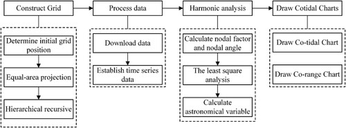
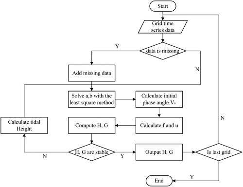
First, using the grid cell as the regional unit, the satellite altimeter data are interpolated into the grid to establish time series tidal data in each unit. Then, using the least square method to extract the harmonic constants of the eight major tides which include four semidiurnal tidal constituents (the M₂, S₂, N₂, K₂) and four diurnal components (K₁, O₁, P₁, Q₁). Finally, the cotidal charts representing tidal features are drawn on the global hexagonal grid. The specific steps are shown in Figure 1.

Figure 1. Technical routine.

4. Methodology

4.1. Constructing global equal-area hexagonal grid

At present, studies of global hexagonal grid are mainly based on octahedron (Bai, 2011) or icosahedron (Bai, Zhao, & Chen, 2005; Zhang, Ben, Tong, & Dai, 2006). In comparison, icosahedron is the smallest polyhedron among several regular polyhedral, which is the closest to the spherical polyhedron. The global discrete grid divided on this basis has relatively small deformation and more uniform geometric properties, which is conducive to global spatial data integration and Earth system model calculation (Lin, Xu, Sheng, Lv, & Zhou, 2016). Therefore, we construct a global hexagonal grid based on icosahedron.

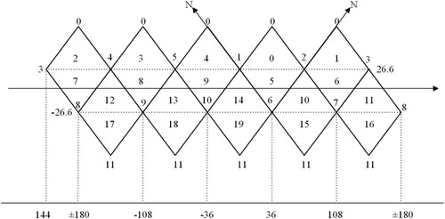
The first step is to determine the correspondence between an icosahedron and the earth’s surface. First, two vertices of an icosahedron are placed on the north and south poles, another vertice is at (0°E, 26.6°N). Second, expand the regular icosahedron and number the vertices and cells, the rules are as follows: the north and south poles are vertex 0, vertex 11, vertex 1 is on the prime meridian, and so on. And the triangle 0–4 is north of 26.6° N, and triangles 5–9 on its common side, the triangle 15–19 is north of 26.6°S, and its co-side is triangles 10–14 (Figure 2).

Figure 2. Vertex and cells coding on an unfolded icosahedron.

In the second step, the grid cells are projected according to the Icosahedron Snyder Equal Area projection (ISEA, Snyder, 1992) method. Unlike triangles and diamonds, which can completely cover the 20 triangles in Figure 2, hexagons cannot completely cover the icosahedral surface, and there must be pentagons on its 12 vertices. Therefore, the initial grid is composed of 12 pentagons.

After determining the initial grid, a global hexagonal grid with an arbitrary resolution can be constructed using hierarchical recursive subdivision, (Figure 3) is a recursive grid generated by DGGRID (Sahr, 2015). In this paper, we use aperture 4 to recursive segmentation, that is, the area of the upper level of grid cells is four times that of the next level. Table 1 provides information about the hexagonal grid.

Figure 3. Spherical hexagonal discrete global based on an icosahedron.

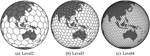
Table 1. Resolution of the global equal-area hexagonal grid.

Level	5	6	7	8	9	10
Resolution (km)	220	110	55	27.5	15.7	7.8
Cell Number	10242	40962	163842	655362	2621442	10485762

4.2. Source and processing of altimeter data

4.2.1. Source of altimeter data

The data used in this paper is the tertiary processing product of satellite data from AVISO in France, distributed by the Copernicus Marine Service. The data has been corrected by the ionospheric correction, dry/wet trospheric correction, electromagnetic bias correction, inverse pressure correction and solid tide, load tide, extreme tide correction. For details, see the quality information document published on its office website (https://catalogue.marine.copernicus.eu/documents/QUID/CMEMS-SL-QUID-008-032-068.pdf).

4.2.2. Processing of altimeter data

To obtain the time series tidal data of the track points, using the nearest neighbour query to find the cell code closest to the track point, and then put the track point into the corresponding hexagonal grid. Since the spacing of hexagonal grid is larger than the spacing of satellite trajectory data, multiple trajectory points will fall into the same grid. To get the average significance of tidal information, we average all altimeter data falling into the cell in the same period, and obtain the time series tidal data in each cell by repeating the operation in all periods. The storage structure of the processed satellite altimeter data is shown in Table 2.

Table 2. Satellite data storage structure after processing.

Cell id	Cell centre	Time series data
Hexagon	(x1, y1)	[[time1,data1], [time2,data2], …]
Lon/lat	(x2, y2)	[[time3,data3], [time4,data4], …]
…	…	[… , … , …]

4.3. Harmonic analysis

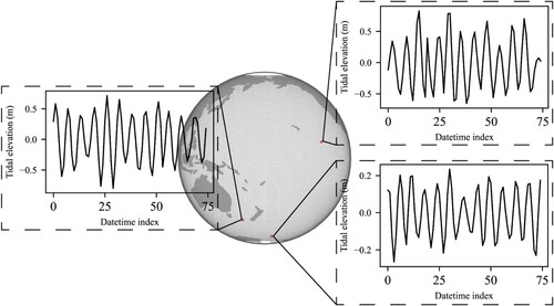
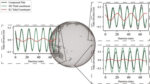
Harmonic analysis is performed to calculate the harmonic constants (amplitudes and phase lags) of the tide constituents along the satellite altimeter tracks. Figure 4 shows the satellite altimeter sequence data of several points in the Pacific Ocean, which can represent oceanic tidal wave characteristics, and the time interval is satellite altimeter cycle. The tidal height at time t of each grid cell is expressed by Equation (1). (1) ${\xi }^{\mathrm{\prime }}\left(t\right)=a_0+\sum _{j=1}^m{f}_j{H}_j\cos \left({\sigma }_{j}t+V_{0j}+u_j-G_j\right)$(1) where a₀ is the mean height, f_j, u_j, ${\sigma }_{\mathrm{j}}$, ${\mathrm{V}}_{0j}$, ${\mathrm{H}}_{\mathrm{j}}$, G_j are the nodal factor, nodal angle, angular speed, astronomical initial phase angle, amplitude and phase lag of jth constituent, m is the total number of tidal components.

Figure 4. Satellite altimeter sequence data of several points.

(2) $R_j=f_j{H}_j{\theta }_j=G_j-V_{0j}+u_j$(2) Due to the correspondence of Equation (2), Equation (1) can be transformed to (3) ${\xi }^{\mathrm{\prime }}\left(t\right)=a_0+\sum _{j=1}^m{R}_j\cos ({\sigma }_{j}t-{\theta }_j)$(3)

Let $a_j$ = $R_j\cos {\theta }_j$ and $b_j$ = $R_j\sin {\sigma }_{j}t$, then (4) ${\xi }^{\mathrm{\prime }}\left(t\right)=a_0+\sum _{j=1}^m(a_j\cos {\sigma }_{j}t+b_j\sin {\sigma }_{j}t)$(4) Using the least square method to solve the harmonic constants of each constituent has become the standard method (Fang, 2016). Let the calculated tide height ${\xi }^{\mathrm{\prime }}\left(t\right)$ approach the measured tide height $\xi \left(\mathrm{t}\right)$. According to the principle of the least square method, then (5) $D={\int }_{-T/2}^{T/2}[\xi \left(t\right)-{\xi }^{\mathrm{\prime }}\left(t\right){]}^2\mathrm{d}t$(5) where T is the total length of the time series. Take the partial derivatives of D with respect a₀, $a_j$, $b_j$ and set them to 0, then we obtain (m + 1) equations. (6) $\{\begin{array}{c}{\alpha }_{00}\ast a_0+{\alpha }_{01}\ast a_1+\dots +{\alpha }_{0m}\ast a_m={\displaystyle \frac{2}{T}\ast {\int }_{-\frac{2}{T}}^{\frac{2}{T}}\xi \left(t\right)\mathrm{d}t}\\ {\alpha }_{10}\ast a_0+{\alpha }_{11}\ast a_1+\dots +{\alpha }_{1m}\ast a_m={\displaystyle \frac{2}{T}\ast {\int }_{-\frac{2}{T}}^{\frac{2}{T}}\xi \left(t\right)\mathrm{d}t}\\ \begin{array}{c}\dots \dots \dots \dots \dots \dots \dots \dots \dots \dots \dots \\ {\alpha }_{m0}\ast a_0+{\alpha }_{m1}\ast a_1+\dots +{\alpha }_{mm}\ast a_m={\displaystyle \frac{2}{T}\ast {\int }_{-\frac{2}{T}}^{\frac{2}{T}}\xi \left(t\right)\mathrm{d}t}\end{array}\end{array}$(6) where ${\alpha }_{00}=2,{\alpha }_{0j}=2\ast \sin \left({\sigma }_j\ast {\displaystyle \frac{2}{T}}\right)/\left({\sigma }_j\ast {\displaystyle \frac{2}{T}}\right)\left(j=1,2,3,\dots ,m\right)$ ${\alpha }_{i0}=2\ast \sin \left({\sigma }_i\ast {\displaystyle \frac{2}{T}}\right)/\left({\sigma }_i\ast {\displaystyle \frac{2}{T}}\right)\left(i=1,2,3,\dots ,m\right)$ ${\alpha }_{ij}=1+2\ast \sin \left({\sigma }_i\ast {\displaystyle \frac{2}{T}}\right)/\left({\sigma }_i\ast {\displaystyle \frac{2}{T}}\right)\left(i=j\right)$ ${\alpha }_{ij}=\sin \left(({\sigma }_i-{\sigma }_j\right)\ast {\displaystyle \frac{2}{T}})/\left(({\sigma }_i-{\sigma }_j\right)\ast {\displaystyle \frac{2}{T}})+\sin (({\sigma }_i+{\sigma }_j)\ast {\displaystyle \frac{2}{T}})/\left(({\sigma }_i+{\sigma }_j\right)\ast {\displaystyle \frac{2}{T}})\left(i\ne j\right)$

m equations are required to compute the coefficient b_j. (7) $\{\begin{array}{c}{\text{β}}_{21}\ast b_1+{\text{β}}_{12}\ast b_2+\dots +{\text{β}}_{1m}\ast b_m={\displaystyle \frac{2}{T}\ast {\int }_{-\frac{2}{T}}^{\frac{2}{T}}\xi \left(t\right)\sin \left({\sigma }_{1}t\right)\mathrm{d}t}\\ {\text{β}}_{21}\ast b_1+{\text{β}}_{22}\ast b_2+\dots +{\text{β}}_{2m}\ast b_m={\displaystyle \frac{2}{T}\ast {\int }_{-\frac{2}{T}}^{\frac{2}{T}}\xi \left(t\right)\sin \left({\sigma }_{2}t\right)\mathrm{d}t}\\ \begin{array}{c}\dots \dots \dots \dots \dots \dots \dots \dots \dots \dots \\ {\text{β}}_{m1}\ast b_1+{\text{β}}_{m2}\ast b_2+\dots +{\text{β}}_{mm}\ast b_m={\displaystyle \frac{2}{T}\ast {\int }_{-\frac{2}{T}}^{\frac{2}{T}}\xi \left(t\right)\sin \left({\sigma }_{m}t\right)\mathrm{d}t}\end{array}\end{array}$(7) where ${\alpha }_{ij}=\sin \left(({\sigma }_i-{\sigma }_j\right)\ast {\displaystyle \frac{2}{T}})/\left(({\sigma }_i-{\sigma }_j\right)\ast {\displaystyle \frac{2}{T}})-\sin (({\sigma }_i+{\sigma }_j)\ast {\displaystyle \frac{2}{T}})/\left(({\sigma }_i+{\sigma }_j\right)\ast {\displaystyle \frac{2}{T}})\left(i\ne j\right)$ ${\text{β}}_{ij}=1-\sin ({\sigma }_i\ast T)/({\sigma }_i\ast T)\left(i=j\right)$

The values of a₀, ${\mathrm{a}}_1$, a₂, … , ${\mathrm{a}}_{\mathrm{m}}$, b₀, ${\mathrm{b}}_1$, b₂, … , ${\mathrm{b}}_{\mathrm{m}}$ are obtained by solving the above equations (6) and (7). Finally, harmonic constants (H_j and G_j) of each tidal component can be calculated by Equation (2). Where the value of initial phase angle ${\mathrm{V}}_{0\mathrm{j}}$ and the nodal factor f_j, nodal angle u_j are calculated from the intermediate time of measured data according to the method of Chen (Chen, Huang, Tang, Zhao, & Wang, 1990).

When solving the least square method, it is necessary to meet equal intervals of tidal data. For satellite altimeter data, there are often cases where data is missing and missed, or other abnormal conditions lead to major errors in some measured data. At present, multiple harmonic analysis methods are often used for processing. In this paper, the missing data is replaced by the value of the last period cycle, and the harmonic analysis is carried out to calculate the harmonic constant, and then use the harmonic constant to inversely calculate the tidal height which to replace the satellite height data, until the calculated harmonic constant does not change anymore.

The harmonic constants of eight major constituents can be obtained by the above procedures, after obtaining the harmonic constants, the sequential tidal height of any sub-tide or compound tide can be calculated according to Formula 1. Figure 5 shows the tidal elevation of compound tide calculated from several points in Figure 4, as well as the tidal elevation of semi-diurnal constituent M₂ and diurnal constituent K₁ with a large proportion of tide.

Figure 5. Schematic diagram of tidal elevation sequence of compound tide and major constituent tides derived from harmonic constants.

The specific process is shown in Figure 6.

Figure 6. Flow chart of calculating harmonic constants.

4.4. Drawing cotidal charts

Cotidal charts is showing the distribution and variation of a tidal wave, consisting of two different contour lines. The points where high tides occur at the same time are connected to form a line, which is the co-tidal line, and the points with equal time difference are connected to form a line, which is the co-range line. The contour lines extracted from the amplitude values are the co-tidal lines, and the contour lines extracted from the phase lag values are the co-range lines, we draw those lines in the global hexagonal grid. The steps for drawing cotidal charts on a global discrete grid include: (1) Interpolating harmonic constants to discrete grids; (2) Search for equivalent grid cells; (3) Visual harmonic constants.

4.4.1. Interpolate harmonic constants to discrete grids

Interpolate the harmonic constant data obtained in Section 4.3, The data interpolation method includes several steps (Figure 7):

1. According to the research scale and the resolution of satellite altimeter data, the appropriate grid resolution level was selected, and the grid types were divided into terrestrial and marine.

2. Determine the grid cell type. Assign the terrestrial cell to None, and if it’s a marine cell and has values, keep the values reserved. Otherwise, it needs to be assigned a value.

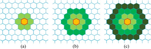
3. For each hexagonal cell, the algorithm searches recursively within its immediate and remote neighbours until at least 4 neighbours have valid values. And then interpolated by the spherical inverse distance weight method.

Figure 7. Schematic diagram of diffusing query adjacent neighbour: (a) first layer diffusion; (b) second layer diffusion; (c) third layer diffusion.

4.4.2. Search for equivalent grid cells

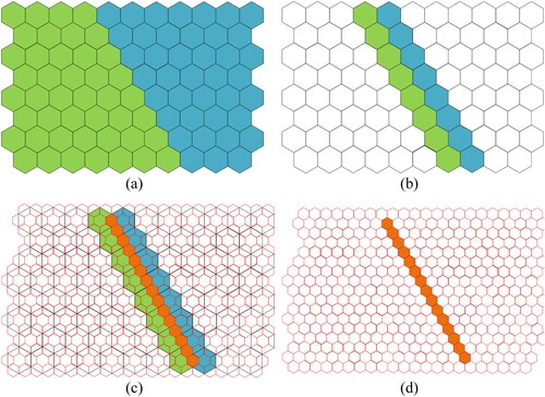
Equivalent retrieval is the process of setting the minimum value and the equivalent spacing reasonably according to the data range, and querying all the equivalent points according to the depth-first traversal. To obtain the grid cell boundaries, this study displays the boundary cells at a higher resolution grid level. It includes the following steps (Figure 8):

1. According to the data range, the minimum value and contour distance of equivalent value are set reasonably to obtain the equivalent list.

2. Grid cell classification. Determine which equivalent interval the value of the point is in, and assign its category code (the code starts from 1).

3. Obtain the grid cells on both sides of the border. According to whether the adjacent cell category is the same, get the cell boundary of different types.

4. Get cell boundaries at a higher resolution grid. Determine the cell index at a higher resolution through the common edges of different categories.

Figure 8. Steps for searching equivalent grids: (a) grid classification; (b) category boundary; (c) query higher level grid boundary; (d) the equivalent grids under higher level grid.

4.4.3. Visual harmonic constants

Through the above two steps can draw the results of harmonic analysis. However, when the contour is drawn, since 0° and 360°are not equal, it’s necessary to calculate the sine and cosine values of phase lag to keep 0° and 360° algebraically equal, and then the phase lag can be calculated by arc tangent value. At the same time, in the classification process, the search range needs to be set as a ring.

Through the above steps, the cotidal charts can be drawn on the spherical hexagonal grid. Figure 9 is the visualization of the harmonic constant of M₂ component of TPXO9.5 tidal model through steps 4.4.1 and 4.4.2.

Figure 9. An example diagram of Cotidal Chart.

TPXO9.5 (Egbert & Erofeeva, 2002) is a global model of ocean tides, which best-fits, in a least-squares sense, the Laplace Tidal Equations and along track averaged data from TOPEX/Poseidon and Jason obtained with OTIS.

5. Case study

The fourth chapter completely introduces the extraction process of ocean tide information based on global hexagonal grid. To evaluate the feasibility of the method, we applied this process to the global ocean, tested the accuracy of harmonic constant extraction by this process through the ocean model, and verified the advantages of the global equal-area hexagonal grid in global tidal information extraction by comparing with the harmonic constant extraction results based on global lat/lon grid.

5.1. Study region and data

In this study, tidal harmonic analysis of satellite altimeter data based on the block method is carried out with global ocean as research area. Due to ocean tides can consider constituents in more than 386, but some small subtidal tides contribute little to tidal height, therefore, we select eight major astronomical constituents for harmonic analysis, including four major semi-diurnal constituents (the M₂, S₂, N₂, K₂) and four major diurnal constituents (Q₁, O₁, K₁, P₁). To overcome the influence of tidal aliasing, we use 19.8 years of satellite altimeter data (as shown in Table 3), which can improve the spatial coverage and time continuity of the altimeter data in the study area. The satellite trajectory distribution of the global ocean is shown in Figure 10.

Figure 10. Jason series satellite ground tracks of global ocean.

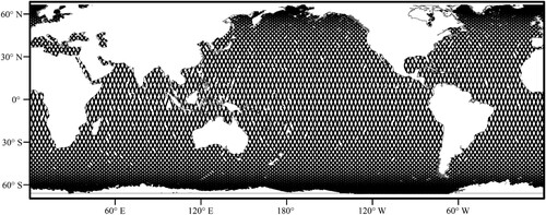
Table 3. Introduction of altimeter data.

Altimeter data	Start time	End time
Jason-1	2002/4	2008/10
Jason-2	2008/10	2016/5
Jason-3	2016/5	2022/2

To compare with the lat/lon grid, we adopt a 6-level grid with resolution close to 1°*1°, which is seamless and non-overlapped. First, the satellite altimetry data is processed according to the method described in Section 4.2.2, and the tidal time series data under the equal-area hexagonal grid is obtained. According to the method described in Section 4.3 of this paper, the harmonic constants of the eight tidal components are obtained through harmonic analysis of the data.

5.2. Validation of harmonic analysis results

5.2.1. Comparison with ocean tidal gauges and ocean model

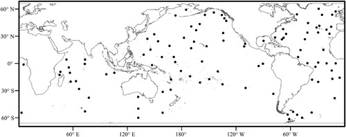
To verify the accuracy of the results, we adopt the gauge stations used in the GOT99.2 model (Ray, 1999) and were used by Shum (Shum et al., 1997) to evaluate the accuracy of dozens of global tidal models. It consists of 102 stations, including 22 stations in the North Atlantic, 19 stations in the South Atlantic, 18 stations in the Indian Ocean, 26 stations in the North Pacific, and 17 stations in the South Pacific. The specific distribution is shown in Figure 11. Most of these tidal gauge stations located in the deep ocean (depth > 1000 m), and the rest of them are on islands.

Figure 11. Location distribution of gauge stations.

The harmonic constants based on the hexagonal grid are interpolated by inverse distance weight method to obtain the data at the tidal gauge stations. Figure 12 shows the results of the harmonic analysis of the M₂ constituent and the results of the TPXO9.5 model in the above 102 stations. Because some points are close to small islands in the model, and extracted as null values, so the actual effective gauge stations are 94.

Figure 12. Comparison of the TPXO9.5 ocean model and simulated results for the tidal constituent M₂.

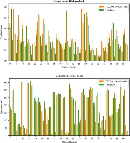
It can be seen from Figure 12 that the results largely agree with the TPXO9.5 tidal ocean model in most oceans all over the word. However, large deviations are observed in the data collected at individual stations. The simulated amplitudes are larger than the tidal ocean model by more than 10 cm measured at stations 63 and 91. The simulated epoch values of the M₂ component are 30° larger than the tidal ocean values at stations 24 and 32.

Table 4 shows the root mean squared error (RMSE) values for the amplitude and phase values simulated using the hexagonal grid in this paper and the TPXO9.5 ocean model, which is defined as (9) $RMSE=\sqrt{{\displaystyle \frac{{\sum }_{i=1}^N{(p_i-O_i)}^2}{N}}}$(9) where N is the number of tidal gauge stations, P_i is the simulated value and O_i is the TPXO9.5 model data. The specific numerical comparison results of eight components are shown in Appendices 1 and 2.

Table 4. RMSE values of eight components at gauge stations.

	RMSE
	H (cm)	G (°)
M2	6.87	10.07
N2	1.5	13.15
K2	1.69	12.77
S2	2.31	12.18
O1	1.48	14.96
P1	1.21	11.89
Q1	0.62	10.97
K1	1.79	9.93

From Table 4, we can see that the RMSE of the amplitude difference is less than 3cm, except for M₂ component. The epoch errors of the N₂ component and the O₁ component are the largest, but they are not more than 15°, which is within the reasonable range of error. In general, the results of the proposed model are consistent with those of the TPXO9.5 global tidal model.

5.2.2. Compare with lat/lon grid

By comparing the results of the harmonic analysis with those of the lat/lon grid to verify the advantages of the equal-area hexagonal discrete grid in extracting tidal information from satellite altimeter. Since the global hexagonal grid with 6 level of resolution is adopted in this paper, the corresponding spatial resolution is 1°. Therefore, the lat/lon grid of 1° is selected for comparative verification experiments. And the position of the comparison points is the 102 tidal gauge stations shown in Figure 11. Appendices 3 and 4 show the absolute error between the calculation results and the TPXO9.5 tidal model under the latitude and longitude grid.

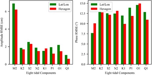
Figure 13 shows the RMSE between the extraction results of the two types of grids and the TPXO9.5 model. As can be seen from the left figure, except for the amplitude of K₁ component, the calculation error of the hexagonal grids is smaller than that of the lat/lon grids in other sub-tides. In the figure on the right, the phase error of the lat/lon grid is slightly smaller than that of the hexagonal grid under N₂ and K₁ components, and the gap is within 1°. However, in the remaining six components, the calculation error of the hexagonal grid is smaller than that of the lat/lon grid, and the error gap reaches 2° under M₂, K₁, P₁ and Q₁ components. Therefore, it can be concluded that the hexagonal grid used in this paper is more suitable for the extraction of global ocean tidal information than the lat/lon grid with the same resolution as the equator.

Figure 13. Comparison of the RMSE for the simulation results obtained using the two grids.

5.3. Result visualization

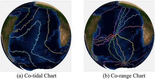
The obtained global ocean harmonic constants are visualized on the cotidal charts of the hexagonal discrete grid. The drawing process is detailed in Section 4.4. In this paper, the M₂ tidal component is taken as an example to draw tide cotidal chart. For M₂ tidal components, the amplitude ranges from 0 to 3, and the values are divided into 16 grades with 0.2 as equivalent spacing, such as the left charts in Figure 14. The phase lag ranges from 0 to 360, and the values are divided into 11 grades with an equivalent interval of 30 degrees. such as the right charts in Figure 14.

Figure 14. Co-tidal Charts and Co-range Charts of M₂ components in three oceans. Left are Co-tidal charts and right are Co-range charts.

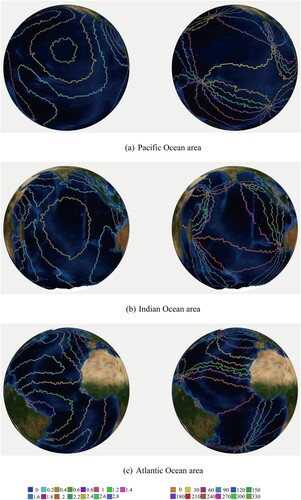
In the figure, the intersection of different co-range lines are the amphiprotic points, that is, the tidal range is very small, which can be regarded as the stable point where the sea surface does not rise or fall. It can be seen from Figure 14 that the M₂ component tide successfully simulated four amphiprotic points in the central Pacific Ocean within 66 degrees north and south latitude, including two amphiprotic points in the North Pacific and two amphiprotic points in the South Pacific. Three amphiprotic points were simulated in the Atlantic region, located east of North America, near the Lesser Andres Islands, and east of South America. Two amphiprotic points are simulated in the Indian Ocean region, located in East Africa and west Australia respectively. All of the amphiprotic points are basically the same as the previous simulation results.

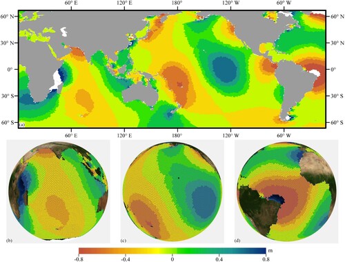
In this paper, the harmonic constants of eight constituents calculated in Section 4.3 are used as the data source for inversion, and the global tide elevation data at any time can be obtained. Figure 15 shows the global tidal elevation at Zero o’clock on October 1, 2002.

Figure 15. Tidal elevation was retrieved from eight major constituents: (a) Global Ocean tidal elevation; (b) Indian Ocean tidal elevation; (c) Pacific Ocean tidal elevation; (d) Atlantic Ocean tidal elevation.

6. Discussion on the advantage of equal grid

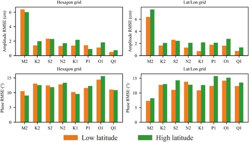
In this paper, the low latitude area is within 30° N/S, and the high latitude area is 30–66°N/S. The experiment in Section 5.2.2 was divided into high latitude and low latitude respectively, RMSE is used as the evaluation index, and the results are presented in Figure 16.

Figure 16. Comparison of RMSE of two types of grid in different latitude intervals.

From the figure, it can be concluded that:

• For hexagonal grid, RMSE values are not significantly different at low and high latitudes, whether amplitude or phase lag. It is not intuitive to see the impact of different latitude intervals on the RMSE value.

• For the lat/lon grid, it can be seen that the amplitude/phase RMSE value in the high latitude is larger than that in the low latitude for the eight components, except for the phase of N₂ tidal component.

Therefore, it can be concluded that the calculation error of the lat/lon grid is larger than that of the hexagonal grid, and the error of the lat/lon grid increases with the increases of latitude. It’s reasonably proved that the change of grid area of the lat/lon grid will affect the result of tidal information calculation with the increasing of latitude, while the equal area grid is not affected by the increase of latitude.

6.1. Discussion on optimal grid resolution

To compare with the lat/lon grid commonly used by researchers, we select a global equal-area hexagonal grid with level 6 of resolution, which corresponding spatial resolution is 1 degree. However, it is also an important part of the experiment to select the most suitable grid resolution for harmonic analysis of global satellite altimeter data, therefore, the resolution of global equal-area hexagonal grid which is most suitable for tidal analysis is discussed in this chapter.

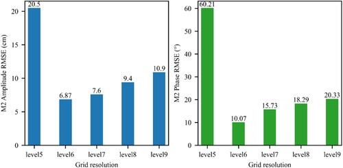
102 tidal gauge stations in Figure 11 are still selected for validation, since the zonal resolution of satellite altimeter data is 5–6 km, experiments are carried out from level 5 to level 10 which is close to the zonal resolution of satellite altimeter data to discuss the optimal grid resolution for processing satellite altimeter. The grid resolution is shown in Table 1.

Due to the highest resolution being level 10 and the deviation between the satellite altimeter data trajectories can reach 1–2 km, it often does not fall into data in 3–4 consecutive periods of satellite, so it cannot be fitted by the least square method. Therefore, we only analyse the harmonic constants calculated based on the levels 5–9. The harmonic constants calculated by each level of grids were obtained by inverse distance interpolation at tidal gauge stations and compared with the harmonic constants of the M₂ component provided by Shum (Shum et al., 1997).

It can be seen from Figure 17 that the RMSE is the smallest under the level 6 grid, whether it is the amplitude or the phase lag. At the same time, the latitude and longitude difference of hexagonal grid at the equator is close to the resolution of 1 degree of the lat/lon grid commonly used by scholars, and the radius length of the hexagonal grid remains the same all over the world, which is more advantageous than the lat/lon grid in processing global data. Therefore, it can be considered that level 6 grid is the optimal resolution for extracting tidal parameter from satellite altimeter data.

Figure 17. RMSE-Amplitude (left), RMSE-Phase (right).

7. Conclusion

This study aims to satisfy the efficient processing of ocean data, analyses the shortcoming of the existing method, and on this basis proposes to use the global equal-area hexagonal grid system as the data frame to realize the tidal information analysis of satellite altimeter data. The conclusions are as follows:

• The global equal-area hexagonal grid provides a basis framework for the expression and processing of a large amount of global marine spatial data. The data does not require multiple transformations and adjustment calculations, which reduces the loss of accuracy and efficiency. The ocean tide information harmonic analysis is carried out by projecting 19.8 years of satellite altimetry data onto the global hexagonal discrete grid, and the results are in accordance with the basic characteristics of eight tidal components.

• By comparing the harmonic constants calculated in the hexagonal grid with those calculated in the lat/lon grid, it can be concluded that equal-area grid has more advantages than the lat/lon grid in processing satellite altimeter data, and the calculation accuracy of equal-area grid is higher than that of the lat/lon grid in the same resolution.

• This paper demonstrates the important influence of equal-area grid in expressing and processing large amounts of satellite trajectory data and provides a new idea for the spatial analysis of ocean data.

Data and availability statement

The data that support the findings of this study are available through the following private link: https://doi.org/10.5281/zenodo.7378937.

Disclosure statement

No potential conflict of interest was reported by the author(s).

Additional information

Funding

This work was supported by the National Natural Science Foundation of China [42076203].

Appendices

Appendix 1

Table

Station			M2		K2		S2		N2
Index	Lon	Lat	△H (cm)	△G (°)	△H (cm)	△G (°)	△H (cm)	△G (°)	△H (cm)	△G (°)
1	−28.8	60.2	6.51	8.79	2.44	4.17	1.40	2.46	1.16	3.83
2	−10.1	57.2	5.35	4.15	6.22	8.80	6.26	1.68	1.27	3.08
3	−52.8	54	0.76	3.05	0.71	8.74	1.41	28.81	0.02	8.69
4	−13.9	53.6	7.10	3.70	4.87	2.49	0.50	3.42	6.19	29.65
5	−25.1	53.5	2.93	4.64	0.15	9.20	2.47	0.22	1.20	1.29
6	−40.5	44.5	1.71	18.61	2.17	13.43	0.83	12.48	0.60	19.00
7	−28	41.4	7.25	1.30	0.44	7.32	1.81	7.13	1.99	2.56
8	−15	40.3	9.45	4.76	0.64	6.57	2.67	9.58	2.12	4.23
9	−31.1	39.5	6.32	0.87	0.94	8.30	1.85	4.51	1.20	2.79
10	−68	37.8	5.69	4.22	2.56	2.94	0.35	8.30	2.29	1.57
11	−20.1	37.2	8.07	4.14	2.03	5.79	1.68	0.70	5.19	9.84
12	−29.4	34	4.82	5.08	0.50	1.96	1.33	6.75	0.44	6.68
13	−41.2	33.9	1.12	4.95	1.68	4.17	1.96	6.55	0.78	2.58
14	−16.9	32.6	5.46	3.89	1.03	2.80	2.21	5.67	0.11	4.65
15	−64.7	32.4	4.86	6.54	1.56	16.76	1.44	6.45	0.72	9.98
16	−76.8	28.5	4.94	6.02	0.17	3.08	1.55	12.96	0.24	2.20
17	−67.5	28.2	4.73	2.40	1.79	4.99	1.09	6.00	0.88	3.51
18	−44	26.6	3.19	6.83	0.41	1.47	0.46	3.91	0.12	3.10
19	−69.3	26.5	4.53	4.33	0.92	2.74	1.00	18.12	0.86	5.82
20	−89.6	24.8	0.04	26.17	0.35	17.09	1.05	29.12	0.04	22.52
22	−48.8	14.7	7.50	23.22	1.14	2.79	2.16	2.14	0.85	17.25
23	−51.5	7	9.76	2.74	1.08	7.18	0.27	14.04	3.59	4.53
24	−29.3	0.9	5.11	38.68	0.76	4.01	3.37	6.21	1.57	4.53
25	−41.2	0.2	3.15	2.79	3.86	7.17	2.67	0.95	0.59	4.25
26	−20	0	8.31	17.79	1.22	9.26	1.50	1.18	1.22	8.83
27	−10	0	5.43	4.34	0.83	2.07	0.12	2.38	0.65	11.02
28	5.6	−1.4	6.72	4.82	0.50	5.01	2.00	1.74	1.20	1.70
29	−32.4	−3.8	10.49	17.82	3.68	4.23	3.00	2.08	0.77	2.03
30	−14.4	−7.9	4.20	5.99	0.40	4.56	0.04	7.91	0.20	24.93
31	−5.7	−15.9	3.62	1.78	0.83	4.13	0.99	8.02	0.20	3.31
32	−13.7	−17.1	3.53	34.02	1.84	24.91	0.59	19.75	0.79	14.32
33	−36.1	−18	9.63	6.28	2.10	0.32	3.77	4.34	0.84	0.12
34	−29.3	−20.5	5.14	3.80	1.27	3.41	1.65	4.30	0.68	12.84
35	−11.1	−38.5	3.39	2.32	0.73	0.34	0.85	4.76	1.38	1.33
36	−57	−53.5	2.45	5.54	0.93	14.88	0.59	7.79	1.19	8.16
37	−36.5	−54.3	0.87	4.02	0.65	4.10	1.61	0.71	0.90	11.39
38	3.3	−54.5	2.44	2.81	1.93	3.75	0.99	1.07	0.03	1.99
39	−63	−56.5	8.73	0.94	0.34	6.31	3.07	20.31	1.20	19.54
40	−52.5	−56.7	7.46	4.18	1.05	28.15	2.52	9.40	0.85	4.98
41	−47.1	−60	5.15	3.30	1.56	15.62	7.70	12.08	0.67	9.88
42	−61.3	−61.5	0.58	2.80	0.72	12.52	3.84	14.17	0.97	15.69
43	52.9	4.2	4.54	0.32	0.28	23.17	2.03	1.12	1.09	8.46
44	73.5	4.2	4.61	15.33	0.53	15.07	1.83	5.28	0.39	5.00
45	73.2	−0.7	7.68	2.54	0.59	2.59	2.49	0.49	0.76	4.56
46	55.5	−4.6	5.61	6.59	0.15	18.21	3.32	2.75	0.43	0.99
47	46.2	−9.4	7.48	8.27	1.67	3.55	7.03	8.15	0.24	11.87
48	105.7	−10.4	6.00	5.73	0.48	14.27	2.41	9.34	2.06	9.27
49	56.7	−10.4	4.29	12.49	1.40	1.00	1.30	8.12	0.73	8.44
50	96.9	−12.1	4.82	6.71	1.24	10.32	0.12	4.55	1.36	7.69
52	63.4	−19.7	5.68	1.35	1.54	14.66	4.69	9.90	1.56	10.89
54	66.8	−28.3	6.23	3.15	1.03	1.52	2.00	0.79	1.67	1.56
55	132	−37	1.22	8.32	0.95	7.96	0.65	1.42	0.35	3.56
56	77.6	−37.9	5.51	4.95	0.61	1.70	1.44	4.72	0.88	2.78
57	132.1	−50	0.93	12.65	0.40	7.21	0.60	4.87	0.04	27.41
58	73.4	−53	0.12	23.68	0.48	24.84	1.09	17.70	2.12	29.20
59	132.1	−60	3.33	8.19	0.08	24.77	2.17	3.49	0.67	1.00
60	−175.1	59.1	8.57	9.81	0.42	20.61	0.28	13.36	0.76	6.57
61	−144.4	56.1	13.41	3.99	4.04	3.58	2.57	4.93	1.69	1.84
62	−154.3	53.4	4.89	11.85	1.54	5.50	2.06	16.08	2.65	14.65
63	−135.6	53.3	12.09	4.72	4.17	13.35	1.66	3.62	0.35	7.13
64	173.2	52.8	0.76	0.16	1.94	26.57	0.29	11.53	1.51	3.21
65	−132.8	49.6	0.04	4.54	3.96	1.36	1.63	4.18	0.08	2.13
66	−130.8	46.8	5.95	9.56	0.94	35.31	2.23	2.26	0.30	21.35
67	−160.1	43.3	4.72	4.27	0.60	14.19	1.17	17.15	0.32	1.02
68	−169.4	40.7	2.46	0.41	0.47	26.50	1.28	21.43	1.20	5.70
69	−164	36.5	2.15	4.48	0.14	7.46	1.58	25.21	1.18	4.52
70	−134.2	33.5	2.70	4.45	2.12	15.05	2.70	0.33	2.48	8.01
71	149.8	32	2.90	24.79	0.21	16.53	1.25	13.15	0.54	36.38
72	−177.4	28.2	1.64	0.27	0.15	31.26	2.00	9.37	2.83	8.37
73	142.2	27.1	6.09	18.59	0.31	27.93	1.00	41.44	0.27	12.47
74	−133.9	25	2.38	1.56	0.98	8.72	0.90	4.55	2.62	13.39
75	154	24.3	1.63	8.10	1.06	7.72	0.21	0.45	0.44	3.82
76	−166.3	23.9	0.20	9.86	1.77	21.13	0.65	37.99	2.75	8.97
77	−109.9	21.5	3.23	3.52	1.96	8.76	3.76	0.20	1.91	7.96
78	166.6	19.3	4.99	11.36	0.55	9.69	2.53	1.33	0.83	15.06
79	−152.5	18.9	5.54	6.47	0.08	4.21	1.79	6.82	0.30	4.74
81	−169.5	16.7	3.24	6.01	0.02	3.89	1.07	8.20	0.20	10.00
82	145.7	15.2	4.17	19.19	0.77	12.98	0.46	20.01	0.04	64.22
83	138.1	9.5	9.48	5.05	0.50	11.62	3.10	13.15	1.76	12.24
84	171.4	7.1	9.28	4.46	2.89	11.36	3.77	0.01	2.56	1.07
85	158.2	7	3.95	12.03	1.74	8.04	2.18	11.08	0.03	41.20
87	172.9	1.4	9.86	3.58	1.47	2.09	4.21	12.75	1.03	0.26
88	−90.3	−0.4	4.20	2.47	2.15	13.95	3.13	8.65	1.74	3.47
89	147.3	−2	1.93	5.28	0.31	16.13	1.10	21.18	0.67	4.33
90	−95	−2.9	5.36	4.03	0.80	1.64	2.04	1.42	1.57	3.23
91	179.2	−8.5	10.71	4.01	2.81	13.24	2.76	0.95	1.72	0.28
93	−170.7	−14.3	6.11	1.99	0.25	11.88	0.92	12.73	0.97	7.35
96	−159.8	−21.2	3.82	1.03	0.02	20.02	0.25	13.34	0.99	1.01
97	−134.9	−23.1	4.16	2.67	0.63	8.37	1.17	11.83	0.91	2.81
98	−109.4	−27.2	2.84	1.52	0.03	2.46	1.04	2.33	0.38	2.37
99	167.9	−29.1	6.16	1.66	1.98	15.01	1.48	8.04	0.72	1.97
100	159.1	−31.5	8.19	6.52	1.47	4.54	2.21	33.05	0.49	5.88
101	−78.8	−33.6	4.35	6.48	0.85	5.11	0.96	7.21	0.34	5.07
102	159	−54.5	1.64	0.17	0.46	0.22	0.09	1.47	1.50	6.53

Appendix 2

Table

Station			K1		O1		P1		Q1
Index	Lon	Lat	△H (cm)	△G (°)	△H (cm)	△G (°)	△H (cm)	△G (°)	△H (cm)	△G (°)
1	−28.8	60.2	0.96	2.67	0.66	11.81	0.16	2.42	0.68	2.74
2	−10.1	57.2	0.96	2.58	0.15	3.89	0.47	11.43	0.81	3.96
3	−52.8	54	1.02	5.38	0.83	8.34	0.25	14.86	1.00	14.99
4	−13.9	53.6	2.92	17.90	0.12	11.61	0.04	14.28	0.74	5.45
5	−25.1	53.5	0.35	6.00	0.19	21.70	0.28	9.10	0.40	20.42
6	−40.5	44.5	0.14	10.59	1.39	14.72	0.43	10.06	0.07	27.43
7	−28	41.4	0.23	14.43	0.43	16.32	0.15	9.13	0.90	1.08
8	−15	40.3	0.04	5.63	0.96	27.67	0.18	7.54	0.04	2.84
9	−31.1	39.5	0.42	8.59	0.02	15.95	0.31	3.58	0.89	10.48
10	−68	37.8	0.18	15.45	0.04	15.59	0.13	15.56	0.64	12.14
11	−20.1	37.2	0.05	7.56	0.04	24.26	0.38	12.83	0.33	2.15
12	−29.4	34	0.23	14.25	0.83	13.43	0.42	14.67	0.74	6.46
13	−41.2	33.9	0.03	14.34	0.21	12.04	0.26	7.78	1.11	20.53
14	−16.9	32.6	0.03	11.54	0.97	14.38	0.28	13.88	0.18	2.91
15	−64.7	32.4	0.33	10.40	0.47	19.21	0.84	16.48	0.66	2.60
16	−76.8	28.5	1.07	10.23	0.97	4.43	0.59	10.83	0.39	12.95
17	−67.5	28.2	0.19	13.68	0.74	17.97	0.58	6.04	0.53	5.33
18	−44	26.6	0.47	18.01	0.60	9.23	0.36	12.34	0.96	11.95
19	−69.3	26.5	1.84	10.51	0.18	14.86	0.38	12.53	0.53	17.89
20	−89.6	24.8	1.98	3.27	0.26	16.66	0.20	9.89	1.48	6.36
22	−48.8	14.7	0.49	3.25	0.04	3.49	0.87	1.47	0.12	6.79
23	−51.5	7	0.36	2.15	0.90	13.51	0.08	8.52	0.00	5.57
24	−29.3	0.9	0.39	6.05	0.11	4.94	0.30	9.72	0.27	26.64
25	−41.2	0.2	0.46	4.33	0.58	22.54	0.25	10.37	0.07	12.87
26	−20	0	0.78	1.92	0.02	6.39	0.05	15.27	0.44	4.57
27	−10	0	0.65	13.53	0.49	18.06	0.72	0.19	0.91	5.81
28	5.6	−1.4	0.10	7.15	0.45	22.49	0.27	3.80	0.81	6.65
29	−32.4	−3.8	0.36	5.40	0.16	12.63	0.34	6.84	0.18	4.02
30	−14.4	−7.9	0.57	7.60	0.06	22.62	0.30	10.97	0.31	1.88
31	−5.7	−15.9	0.31	11.82	0.21	7.37	0.12	6.60	0.08	3.87
32	−13.7	−17.1	0.46	15.48	0.40	6.69	0.21	9.99	1.00	2.18
33	−36.1	−18	0.04	4.15	1.29	17.31	0.17	14.32	0.20	7.90
34	−29.3	−20.5	0.18	3.45	0.94	6.01	0.09	12.61	0.13	5.32
35	−11.1	−38.5	0.10	7.04	1.18	2.06	0.37	10.90	0.99	3.32
36	−57	−53.5	0.80	1.73	1.43	20.77	0.12	21.63	0.33	10.14
37	−36.5	−54.3	0.35	7.82	0.63	17.88	0.35	4.45	0.03	2.19
38	3.3	−54.5	0.22	10.49	2.32	16.73	0.56	17.96	0.15	2.09
39	−63	−56.5	0.88	4.44	0.92	1.01	2.13	19.18	2.11	6.12
40	−52.5	−56.7	1.75	12.63	0.67	10.59	0.03	5.64	0.23	0.40
41	−47.1	−60	5.38	18.39	0.28	9.36	0.07	6.35	2.65	6.85
42	−61.3	−61.5	6.19	14.68	1.81	7.04	0.11	18.10	0.20	4.61
43	52.9	4.2	0.50	0.64	0.80	19.54	0.32	7.79	0.28	11.38
44	73.5	4.2	1.55	10.39	0.06	24.31	1.00	4.83	0.57	3.97
45	73.2	−0.7	0.49	17.20	0.35	15.37	0.33	20.21	0.03	8.11
46	55.5	−4.6	0.38	16.52	0.73	11.16	1.14	8.91	0.01	1.02
47	46.2	−9.4	0.95	11.19	3.15	13.62	0.03	12.26	0.25	10.19
48	105.7	−10.4	0.38	1.17	0.14	15.30	0.51	21.99	0.34	1.48
49	56.7	−10.4	0.60	6.46	1.16	5.75	0.19	2.00	0.07	0.87
50	96.9	−12.1	1.33	0.24	0.57	12.37	0.33	8.55	0.19	9.20
52	63.4	−19.7	0.12	0.92	0.80	14.76	0.51	18.10	0.18	5.20
54	66.8	−28.3	0.58	13.66	0.18	12.14	0.87	16.22	0.27	3.92
55	132	−37	0.45	10.07	1.07	19.63	0.95	10.06	1.08	11.20
56	77.6	−37.9	0.44	10.43	0.59	10.30	1.34	13.82	0.07	9.65
57	132.1	−50	0.39	4.01	0.50	8.26	0.01	8.59	0.28	9.68
58	73.4	−53	6.50	7.91	0.33	23.35	1.15	18.78	0.21	12.05
59	132.1	−60	2.69	11.27	2.87	5.44	0.87	19.37	0.76	1.39
60	−175.1	59.1	5.32	10.05	2.96	15.88	1.06	1.90	0.11	11.02
61	−144.4	56.1	0.22	5.36	4.27	19.23	0.25	0.69	0.01	3.84
62	−154.3	53.4	0.25	5.15	2.36	28.64	0.61	11.50	0.15	14.13
63	−135.6	53.3	1.01	1.57	2.87	7.09	0.82	1.27	0.86	11.59
64	173.2	52.8	1.95	10.86	4.46	20.17	1.74	8.32	0.27	14.66
65	−132.8	49.6	2.43	7.01	3.09	5.08	0.51	12.05	0.04	7.18
66	−130.8	46.8	3.79	14.58	5.67	0.10	0.75	20.52	0.17	1.97
67	−160.1	43.3	0.11	0.64	0.91	18.60	0.03	20.18	0.43	5.96
68	−169.4	40.7	0.59	8.40	0.20	19.86	1.42	18.94	0.00	7.54
69	−164	36.5	0.64	0.79	0.72	21.65	0.53	18.72	0.27	9.94
70	−134.2	33.5	0.62	10.38	2.09	18.10	2.20	22.67	0.84	31.62
71	149.8	32	3.89	1.25	0.98	4.77	2.73	12.23	0.14	1.81
72	−177.4	28.2	0.03	1.50	2.79	18.98	3.72	10.00	0.00	15.88
73	142.2	27.1	4.85	6.22	1.21	11.18	1.88	16.77	0.17	5.45
74	−133.9	25	1.00	4.76	2.09	18.67	1.88	18.45	0.64	2.24
75	154	24.3	4.74	10.08	0.15	4.03	3.29	9.62	0.26	0.31
76	−166.3	23.9	1.98	17.36	0.63	4.49	1.89	0.10	0.10	6.58
77	−109.9	21.5	1.88	13.79	1.64	12.31	1.43	20.49	0.05	2.09
78	166.6	19.3	1.37	1.61	1.08	3.18	4.83	9.33	0.47	4.25
79	−152.5	18.9	1.89	13.87	1.37	24.52	0.10	17.50	0.29	41.24
81	−169.5	16.7	1.06	13.62	1.32	6.99	2.38	1.48	0.18	1.46
82	145.7	15.2	2.61	8.75	1.07	13.82	1.24	5.83	0.33	7.81
83	138.1	9.5	1.76	8.71	0.98	13.09	0.06	7.68	0.04	7.14
84	171.4	7.1	0.68	3.71	0.16	1.04	3.51	5.71	0.31	10.60
85	158.2	7	1.38	15.15	1.84	16.59	1.20	8.79	0.52	19.07
87	172.9	1.4	0.43	8.97	0.67	2.73	2.85	0.41	0.23	0.69
88	−90.3	−0.4	0.62	8.50	0.09	3.17	0.84	0.18	0.18	4.91
89	147.3	−2	2.18	14.91	3.04	15.39	1.58	0.46	0.27	7.51
90	−95	−2.9	0.46	1.32	0.30	17.75	1.24	0.89	1.77	7.25
91	179.2	−8.5	0.13	18.92	1.15	12.16	0.42	4.82	0.21	20.49
93	−170.7	−14.3	0.33	1.34	0.73	11.97	0.16	8.08	0.37	8.83
96	−159.8	−21.2	0.29	18.80	0.36	23.61	0.14	7.93	0.47	1.38
97	−134.9	−23.1	0.21	7.22	0.43	6.25	0.23	4.55	0.20	5.70
98	−109.4	−27.2	0.63	12.40	1.04	25.75	0.44	6.63	0.00	14.05
99	167.9	−29.1	0.33	4.96	1.35	14.53	1.35	7.66	0.00	20.32
100	159.1	−31.5	0.70	0.84	0.39	12.80	0.24	2.17	0.32	4.63
101	−78.8	−33.6	0.07	0.87	1.48	17.95	1.37	0.14	0.26	2.48
102	159	−54.5	0.13	9.09	1.09	2.04	0.83	12.79	0.13	14.75

Appendix 3

Table

Station			M2		K2		S2		N2
Index	Lon	Lat	△H (cm)	△G (°)	△H (cm)	△G (°)	△H (cm)	△G (°)	△H (cm)	△G (°)
1	−28.8	60.2	6.49	6.15	2.14	7.74	1.76	1.78	0.68	5.60
2	−10.1	57.2	8.03	7.05	6.21	1.12	6.04	7.10	2.59	1.75
3	−52.8	54	8.78	6.51	1.33	9.39	1.17	49.05	0.57	1.21
4	−13.9	53.6	11.44	1.89	4.89	9.24	2.32	8.22	6.58	26.82
5	−25.1	53.5	3.71	4.46	0.28	0.49	1.86	0.42	1.49	1.86
6	−40.5	44.5	2.59	3.61	3.41	8.89	0.49	6.37	3.53	1.00
7	−28	41.4	6.86	4.50	0.47	2.18	2.24	2.62	2.20	4.75
8	−15	40.3	9.94	4.58	0.77	4.72	0.88	4.14	1.63	9.79
9	−31.1	39.5	4.76	3.33	0.97	10.30	1.85	5.99	1.22	4.89
10	−68	37.8	7.72	4.09	3.07	2.71	0.51	13.88	2.98	7.95
11	−20.1	37.2	10.63	3.11	2.13	3.53	1.94	5.97	5.48	6.15
12	−29.4	34	5.28	4.31	0.46	0.29	1.31	5.50	0.44	3.42
13	−41.2	33.9	3.86	3.62	1.80	5.50	1.61	4.58	0.89	2.94
14	−16.9	32.6	8.18	3.11	1.20	3.49	2.61	0.72	0.83	7.36
15	−64.7	32.4	6.13	2.73	2.94	5.33	0.82	20.26	1.72	2.90
16	−76.8	28.5	4.00	0.04	0.25	16.50	0.28	14.27	2.91	0.32
17	−67.5	28.2	5.13	3.97	3.13	16.66	0.21	1.26	1.12	8.26
18	−44	26.6	0.83	3.54	0.44	4.49	0.22	3.20	3.33	2.47
19	−69.3	26.5	4.19	3.51	1.25	20.63	0.25	3.18	1.01	6.02
20	−89.6	24.8	0.22	7.43	0.36	14.54	2.32	21.55	0.07	1.47
21	−23.5	14.9	17.31	24.72	0.33	4.63	1.74	33.21	0.34	2.13
22	−48.8	14.7	5.00	4.42	1.15	4.63	1.55	13.70	0.89	2.52
23	−51.5	7	5.55	4.45	1.09	4.79	0.34	3.24	2.95	5.68
24	−29.3	0.9	11.92	10.65	2.91	3.29	2.65	2.66	3.14	6.71
25	−41.2	0.2	11.07	1.62	3.95	1.56	2.59	2.55	0.01	1.50
26	−20	0	8.54	2.75	1.41	9.43	1.79	3.23	1.95	5.75
27	−10	0	4.06	8.93	0.62	1.27	0.17	9.29	0.81	13.79
28	5.6	−1.4	7.23	4.50	0.69	5.60	1.31	1.04	3.27	5.51
29	−32.4	−3.8	10.97	21.01	3.81	1.03	3.03	5.02	2.32	3.69
30	−14.4	−7.9	3.71	2.55	0.23	4.71	0.41	1.86	0.18	10.03
31	−5.7	−15.9	3.80	2.59	0.73	1.85	1.27	3.87	0.02	5.66
32	−13.7	−17.1	1.53	11.65	1.74	1.77	1.19	10.78	3.52	14.71
33	−36.1	−18	8.41	6.11	2.16	0.75	2.87	1.32	2.88	4.06
34	−29.3	−20.5	5.68	4.11	1.33	5.73	0.74	1.33	0.50	9.37
35	−11.1	−38.5	2.72	3.13	0.81	3.26	0.82	7.36	1.26	0.02
36	−57	−53.5	2.44	0.87	0.77	2.67	1.00	7.83	1.45	30.57
38	3.3	−54.5	4.95	3.46	2.14	4.33	0.37	7.70	0.13	1.11
39	−63	−56.5	3.78	2.05	0.18	3.08	2.19	0.83	2.68	4.95
40	−52.5	−56.7	3.74	4.81	0.85	26.08	1.88	5.33	2.03	3.06
41	−47.1	−60	10.48	0.64	1.34	7.52	8.50	20.47	2.67	29.70
42	−61.3	−61.5	0.55	7.07	1.51	2.09	3.60	3.21	0.72	19.11
43	52.9	4.2	4.42	3.68	0.27	0.62	2.30	0.56	1.26	9.78
44	73.5	4.2	7.27	12.52	0.64	1.46	2.74	4.08	2.83	27.27
45	73.2	−0.7	6.26	1.04	0.50	2.95	2.62	1.63	1.17	9.37
46	55.5	−4.6	9.39	8.24	0.16	36.58	3.02	1.68	1.24	1.06
47	46.2	−9.4	3.93	6.88	1.65	2.12	6.74	6.90	0.58	0.58
48	105.7	−10.4	0.70	17.03	0.33	6.37	2.26	6.29	1.82	7.10
49	56.7	−10.4	4.11	3.10	1.42	38.59	1.60	14.16	0.53	6.10
50	96.9	−12.1	4.29	5.16	1.37	16.60	0.65	12.71	1.18	13.71
51	45.3	−12.8	8.13	2.91	0.59	17.69	10.89	20.99	1.29	4.63
52	63.4	−19.7	4.09	1.96	2.49	20.60	4.46	24.98	1.36	3.34
54	66.8	−28.3	4.69	6.25	2.96	4.49	1.59	2.00	1.59	7.33
55	132	−37	1.79	3.18	0.90	5.73	0.46	3.92	2.64	15.60
56	77.6	−37.9	5.05	4.13	0.53	7.03	1.47	0.55	1.97	5.25
57	132.1	−50	1.10	1.79	0.43	6.64	0.50	1.65	0.22	15.45
58	73.4	−53	1.16	32.59	0.59	19.88	2.09	0.74	2.20	38.48
59	132.1	−60	1.62	2.45	0.07	5.30	1.11	0.37	0.81	2.32
60	−175.1	59.1	4.08	4.99	0.51	31.68	0.39	19.59	0.12	2.11
61	−144.4	56.1	14.98	4.09	3.45	30.13	3.03	23.18	2.25	9.42
62	−154.3	53.4	8.98	6.10	2.13	9.62	3.59	34.98	2.19	12.32
63	−135.6	53.3	28.78	22.07	3.48	22.27	4.21	28.44	0.06	1.55
64	173.2	52.8	1.04	0.76	2.52	15.42	0.60	5.04	1.45	3.62
65	−132.8	49.6	9.57	4.13	2.31	16.03	1.69	7.99	0.18	6.94
66	−130.8	46.8	8.37	3.01	1.30	23.32	0.70	2.01	0.16	9.86
67	−160.1	43.3	3.49	4.85	0.42	1.35	1.10	9.78	0.59	6.15
68	−169.4	40.7	2.36	4.70	0.49	22.44	0.75	15.95	0.98	6.97
69	−164	36.5	2.17	3.26	0.20	9.56	0.97	21.33	1.12	1.46
70	−134.2	33.5	3.40	2.29	3.49	22.04	4.22	1.88	2.70	27.00
71	149.8	32	2.33	23.38	1.68	3.61	0.33	9.42	0.51	15.39
72	−177.4	28.2	2.41	2.56	0.05	31.54	1.64	4.29	2.81	1.48
73	142.2	27.1	5.53	2.80	1.13	7.87	0.70	2.73	0.51	5.45
74	−133.9	25	1.69	9.35	1.25	9.23	0.19	0.49	2.91	6.89
75	154	24.3	1.87	6.84	2.44	9.64	0.21	0.68	0.42	25.02
76	−166.3	23.9	0.88	4.39	1.68	17.12	1.41	20.83	2.88	1.77
77	−109.9	21.5	5.32	7.95	2.60	7.54	4.72	0.23	1.56	6.84
78	166.6	19.3	4.29	2.14	0.26	1.42	1.21	0.71	0.72	0.14
79	−152.5	18.9	2.91	2.12	0.12	6.96	1.12	0.11	0.49	0.12
80	−111	18.7	5.48	6.59	2.36	7.49	3.38	4.39	1.31	6.24
81	−169.5	16.7	2.53	4.48	0.18	9.84	1.20	6.87	0.35	8.53
82	145.7	15.2	2.85	6.28	3.10	9.56	1.99	19.99	1.18	9.11
83	138.1	9.5	8.86	3.35	0.21	16.81	2.44	20.79	2.61	5.08
84	171.4	7.1	10.11	2.98	3.70	0.22	1.81	3.35	0.18	10.00
85	158.2	7	4.58	6.99	1.51	5.75	2.17	7.08	0.04	12.89
86	−157.5	2	4.49	4.38	0.29	10.37	0.68	7.54	0.96	0.53
87	172.9	1.4	12.07	5.05	1.33	9.93	2.35	7.85	0.65	5.89
88	−90.3	−0.4	9.58	6.48	2.04	12.46	3.19	13.13	1.38	8.46
89	147.3	−2	2.05	4.68	0.49	21.52	3.20	15.44	1.92	1.17
90	−95	−2.9	6.92	5.08	0.70	4.89	1.86	4.60	1.71	5.33
91	179.2	−8.5	10.44	8.63	2.75	2.07	3.05	7.23	1.02	63.36
93	−170.7	−14.3	2.08	4.28	0.07	10.06	0.57	5.25	0.77	24.61
94	−149.5	−17.5	0.70	2.25	0.10	12.35	0.19	17.58	0.15	10.38
96	−159.8	−21.2	3.91	4.06	0.14	0.02	0.34	1.25	0.83	6.80
97	−134.9	−23.1	4.80	3.06	0.66	19.00	0.88	4.69	1.76	3.60
98	−109.4	−27.2	2.69	2.58	0.04	3.44	0.77	4.91	1.24	2.19
99	167.9	−29.1	5.64	4.70	0.96	6.50	0.87	6.20	0.97	4.81
100	159.1	−31.5	8.18	4.64	1.43	0.26	1.97	11.45	0.56	1.94
101	−78.8	−33.6	4.35	6.26	0.81	9.95	1.14	7.76	1.22	6.29
102	159	−54.5	2.74	7.63	0.43	0.64	0.91	15.59	1.85	7.84

Appendix 4

Table

Station			K1		P1		O1		Q1
Index	Lon	Lat	△H (cm)	△G (°)	△H (cm)	△G (°)	△H (cm)	△G (°)	△H (cm)	△G (°)
1	−28.8	60.2	0.41	7.60	0.29	9.30	1.14	16.53	0.43	9.58
2	−10.1	57.2	0.86	0.38	0.48	7.10	0.52	2.45	1.16	9.65
3	−52.8	54	0.52	6.41	0.58	9.43	0.44	14.96	0.90	14.99
4	−13.9	53.6	2.10	11.92	1.01	10.68	2.47	5.17	1.05	10.11
5	−25.1	53.5	2.12	4.35	0.17	12.93	0.29	22.15	0.15	8.44
6	−40.5	44.5	0.23	9.98	1.44	21.58	1.44	14.33	0.46	8.19
7	−28	41.4	2.00	6.53	1.07	12.09	1.56	12.88	0.71	4.91
8	−15	40.3	0.35	8.16	0.15	5.95	1.21	25.92	0.21	4.91
9	−31.1	39.5	2.14	4.00	1.21	4.50	2.10	16.70	0.72	13.46
10	−68	37.8	2.84	7.20	1.75	13.74	0.38	11.67	0.62	6.07
11	−20.1	37.2	0.14	7.69	0.58	13.02	0.16	15.49	0.12	2.41
12	−29.4	34	0.20	15.03	1.35	11.26	1.32	17.52	0.58	7.00
13	−41.2	33.9	0.00	0.59	2.18	6.57	2.07	0.01	1.00	17.69
14	−16.9	32.6	0.26	11.13	0.26	21.44	1.03	11.15	0.02	2.42
15	−64.7	32.4	2.78	13.57	1.75	19.00	0.05	27.14	0.64	7.67
16	−76.8	28.5	1.02	13.11	1.38	10.01	0.36	1.37	0.40	10.14
17	−67.5	28.2	1.59	22.11	1.51	4.59	0.29	22.81	0.52	14.15
18	−44	26.6	0.58	17.88	2.30	12.17	0.91	10.74	0.69	9.23
19	−69.3	26.5	1.38	22.00	1.35	13.96	0.38	22.20	0.53	10.50
20	−89.6	24.8	0.96	8.72	0.18	9.31	5.72	9.06	1.46	9.65
21	−23.5	14.9	0.66	14.88	0.55	4.82	0.42	22.96	0.17	21.43
22	−48.8	14.7	0.20	10.00	0.83	9.77	1.13	3.00	0.28	10.90
23	−51.5	7	0.14	7.19	0.10	11.36	0.20	9.39	0.02	17.58
24	−29.3	0.9	0.41	9.59	0.25	9.69	0.23	3.08	0.20	17.71
25	−41.2	0.2	0.35	11.55	0.27	5.65	1.91	29.33	0.11	6.72
26	−20	0	0.10	1.80	0.01	15.67	0.15	7.01	0.34	12.55
27	−10	0	0.38	10.91	0.74	0.64	0.74	14.52	0.49	2.58
28	5.6	−1.4	0.04	12.49	1.23	1.78	0.68	25.26	0.66	12.48
29	−32.4	−3.8	0.33	9.51	0.30	3.04	0.31	15.25	0.12	2.68
30	−14.4	−7.9	0.04	14.05	0.26	21.94	0.19	18.91	0.21	3.20
31	−5.7	−15.9	0.13	9.22	0.84	7.84	0.13	1.22	0.38	9.63
32	−13.7	−17.1	0.06	14.55	1.16	13.11	0.02	2.55	0.32	0.46
33	−36.1	−18	0.03	1.64	0.78	27.06	0.26	14.50	0.54	2.12
34	−29.3	−20.5	0.20	10.66	0.85	10.78	0.76	2.67	0.18	7.40
35	−11.1	−38.5	0.11	8.00	1.30	10.77	0.40	1.77	0.84	14.08
36	−57	−53.5	1.19	0.18	0.92	28.71	6.87	13.59	2.31	17.65
38	3.3	−54.5	0.23	16.23	0.47	17.95	2.60	4.08	0.20	10.92
39	−63	−56.5	0.30	10.12	2.16	13.38	6.41	0.52	2.08	2.35
40	−52.5	−56.7	0.22	11.52	1.10	21.66	6.90	9.98	2.22	13.54
41	−47.1	−60	4.73	21.66	2.00	10.48	0.01	9.30	2.64	7.79
42	−61.3	−61.5	1.99	14.46	3.94	23.88	2.28	12.56	3.17	11.26
43	52.9	4.2	1.10	0.34	4.08	7.29	0.45	14.61	1.44	10.91
44	73.5	4.2	1.11	19.75	1.24	9.90	1.87	19.71	0.46	4.63
45	73.2	−0.7	0.27	11.00	1.91	24.83	1.95	0.51	0.54	0.65
46	55.5	−4.6	0.72	18.30	1.91	19.49	1.12	3.89	0.73	0.48
47	46.2	−9.4	0.69	12.97	1.79	12.88	3.55	0.02	0.76	3.45
48	105.7	−10.4	0.80	19.09	0.27	19.25	0.20	17.08	0.31	9.91
49	56.7	−10.4	0.13	19.16	0.02	7.60	1.18	10.35	0.03	1.15
50	96.9	−12.1	1.91	3.06	0.56	6.52	0.16	7.26	0.20	14.40
51	45.3	−12.8	2.03	15.93	1.19	1.91	3.17	4.84	0.59	14.36
52	63.4	−19.7	0.09	2.85	1.69	22.15	1.36	12.84	1.13	17.61
54	66.8	−28.3	0.61	3.52	1.05	3.53	0.89	10.42	1.26	7.13
55	132	−37	0.50	11.24	0.73	4.90	1.94	27.76	0.96	24.86
56	77.6	−37.9	0.20	14.90	1.51	15.09	1.05	18.02	0.96	20.37
57	132.1	−50	0.60	4.86	0.18	14.34	1.26	8.56	0.44	21.43
58	73.4	−53	7.09	13.63	1.04	15.39	3.59	1.72	0.24	14.81
59	132.1	−60	0.57	18.46	1.71	21.70	2.34	12.02	1.61	12.38
60	−175.1	59.1	5.43	5.19	1.72	4.39	1.57	9.11	1.34	9.78
61	−144.4	56.1	2.15	4.77	4.72	5.98	1.56	12.39	2.13	5.08
62	−154.3	53.4	3.16	5.68	4.03	13.83	0.87	21.97	1.98	4.97
63	−135.6	53.3	3.01	4.55	5.21	3.96	2.00	4.82	2.24	5.62
64	173.2	52.8	5.18	15.46	2.06	8.74	2.91	15.61	2.54	12.71
65	−132.8	49.6	0.89	13.44	4.84	17.27	6.95	7.93	2.03	29.53
66	−130.8	46.8	0.08	11.47	4.55	22.13	6.24	0.71	1.90	8.20
67	−160.1	43.3	0.14	0.39	0.30	21.94	1.81	20.09	0.56	22.98
68	−169.4	40.7	0.45	12.03	1.09	19.30	1.11	30.92	0.16	34.74
69	−164	36.5	0.12	0.37	1.27	22.36	0.33	18.95	0.14	16.44
70	−134.2	33.5	1.19	10.22	2.36	20.97	2.52	20.33	0.90	6.24
71	149.8	32	0.01	0.48	2.67	21.70	0.26	2.85	0.00	6.97
72	−177.4	28.2	0.34	3.53	3.44	17.07	2.62	28.76	0.95	9.40
73	142.2	27.1	0.49	16.35	1.88	19.73	0.17	13.68	0.06	15.93
74	−133.9	25	1.31	10.00	1.96	20.81	2.25	29.67	0.68	15.00
75	154	24.3	0.41	21.17	3.38	13.20	1.32	3.63	0.66	1.26
76	−166.3	23.9	0.94	19.95	1.70	1.27	0.98	6.22	0.78	4.83
77	−109.9	21.5	0.75	13.47	1.42	13.38	3.41	14.89	0.94	0.14
78	166.6	19.3	0.61	3.48	4.98	6.43	2.48	1.93	1.42	2.03
79	−152.5	18.9	0.75	9.90	0.18	17.68	0.95	19.83	0.22	24.11
80	−111	18.7	0.50	10.32	0.77	13.63	2.69	4.08	0.68	27.11
81	−169.5	16.7	0.64	17.42	2.25	0.74	1.85	4.64	1.08	3.31
82	145.7	15.2	0.60	11.73	1.37	8.92	0.10	0.05	0.29	13.21
83	138.1	9.5	0.78	10.91	0.22	10.72	0.37	9.25	0.06	5.39
84	171.4	7.1	0.16	8.22	3.78	13.58	0.89	5.80	1.33	5.01
85	158.2	7	1.03	16.56	1.44	7.73	0.88	14.70	0.54	15.18
86	−157.5	2	0.51	14.82	1.04	12.28	0.23	3.81	0.73	7.46
87	172.9	1.4	0.36	7.86	3.17	21.29	0.04	6.59	1.28	5.33
88	−90.3	−0.4	0.30	15.07	0.94	2.68	3.70	22.92	1.21	10.13
89	147.3	−2	0.23	11.31	1.33	5.93	2.79	3.47	0.22	23.15
90	−95	−2.9	0.39	0.18	1.35	4.18	0.36	13.48	1.39	13.56
91	179.2	−8.5	0.10	19.29	2.95	5.85	0.59	26.12	1.30	21.90
93	−170.7	−14.3	0.82	6.65	0.90	13.22	0.72	5.50	0.35	13.62
94	−149.5	−17.5	0.80	5.74	2.51	11.54	1.04	2.08	0.71	8.44
96	−159.8	−21.2	0.15	20.62	1.35	0.31	0.18	26.93	0.47	3.74
97	−134.9	−23.1	0.11	7.96	1.92	4.91	0.89	3.47	0.82	6.90
98	−109.4	−27.2	0.44	0.38	0.58	5.30	0.61	13.35	0.63	24.52
99	167.9	−29.1	0.10	6.91	1.68	6.84	1.77	10.31	1.36	22.10
100	159.1	−31.5	0.10	8.93	0.55	13.13	0.36	9.03	0.46	3.53
101	−78.8	−33.6	0.27	19.65	1.31	18.95	1.44	12.61	0.23	0.63
102	159	−54.5	0.73	12.44	1.07	13.73	0.98	22.66	0.30	9.70

References

- Amiri, Ali Mahdavi, Faramarz Samavati, and Perry Peterson. 2015. “Categorization and Conversions for Indexing Methods of Discrete Global Grid Systems.” ISPRS International Journal of Geo-Information 4 (1): 320–336. doi:10.3390/ijgi4010320.
- Arbic, Brian K., Jerry X. Mitrovica, Douglas R. Macayeal, and Glenn A. Milne. 2008. “On the Factors Behind Large Labrador Sea Tides During the Last Glacial Cycle and the Potential Implications for Heinrich Events.” Paleoceanography 23: 3. doi:10.1029/2007PA001573.
- Bai, Jianjun. 2011. “Location Coding and Indexing Aperture 4 Hexagonal Discrete Global Grid Based on Octahedron.” Journal of Remote Sensing 15 (6): 1125–1137. doi:10.11834/jrs.20110367.
- Bai, Jianjun, Xuesheng Zhao, and Jun Chen. 2005. “Indexing of Discrete Global Grids Using Linear Quadtree.” Geomatics and Information Science of Wuhan University 30 (9): 805–808.
- Bao, Jingyang. 2002. “Study on Tide Analysis Theory and Method Based on Satellite Altimetry Data.” (PhD diss.). Wuhan University.
- Bao, Jingyang, Dingbo Chao, and Jiancheng Li. 2000. “Tidal Harmonic Analysis Near Crossovers of Topex/Poseidon Ground Track in South China Sea.” Acta Geodaetica et Cartographica Sinica 29 (1): 17–23.
- Bao, Jingyang, Dingbo Chao, Jiancheng Li, and Xiaoli Deng. 1999. “A Preliminary Study of the Establishment of Ocean Tide Models in South China Sea from T/P Altimetry.” Journal of Wuhan Technical University of Surveying and Mapping 24 (4): 341–345. doi:10.13203/j.whugis1994.04.012.
- Ben, Jin, Xiaochong Tong, Yongsheng Zhang, and Heng Zhang. 2006. “Snyder Equal-Area Map Projection for Polyhedral Globes.” Geomatics and Information Science of Wuhan University 31 (10): 900–903.
- Bernier, N. B., and K. R. Thompson. 2007. “Tide-Surge Interaction Off the East Coast of Canada and Northeastern United States.” Journal of Geophysical Research: Oceans 112 (C6): 1–12. doi:10.1029/2006JC003793.
- Cartwright, David E., and Richard D. Ray. 1991. “Energetics of Global Ocean Tides from Geosat Altimetry.” Journal of Geophysical Research: Oceans 96 (C9): 16897–16912. doi:10.1029/91JC01059.
- Chen, Zongyong, Zuke Huang, Enxiang Tang, Tianhua Zhao, and Yuzhou Wang. 1990. “A J, V Model for Tidal Analysis and Calculation.” Acta Oceanologica Sinica 12 (6): 693–703.
- Cheng, Yongcun, and Ole Baltazar Andersen. 2011. “Multimission Empirical Ocean Tide Modeling for Shallow Waters and Polar Seas.” Journal of Geophysical Research: Oceans 116 (C11): 1–11. doi:10.1029/2011JC007172.
- Cheng, Yongcun, and Ole Baltazar Andersen. 2017. “Towards Further Improving DTU Global Ocean Tide Model in Shallow Waters and Polar Seas.” Paper presented at the Ocean Surface Topography Science Team Meeting, Miami, FL, USA.
- Desai, Shailen D., and John M. Wahr. 1995. “Empirical Ocean Tide Models Estimated from Topex/Poseidon Altimetry.” Journal of Geophysical Research: Oceans 100 (C12): 25205–25228. doi:10.1029/95JC02258.
- Dutton, Geoffrey. 1984. “Part 4: Mathematical, Algorithmic and Data Structure Issues: Geodesic Modelling of Planetary Relief.” Cartographica: The International Journal for Geographic Information and Geovisualization 21 (2–3): 188–207. doi:10.3138/R613-191U-7255-082N.
- Egbert, Gary D., and Svetlana Y. Erofeeva. 2002. “Efficient Inverse Modeling of Barotropic Ocean Tides.” Journal of Atmospheric and Oceanic Technology 19 (2): 183–204. doi:10.1175/1520-0426(2002)019.
- Egbert, Gary D., and Richard D. Ray. 2000. “Significant Dissipation of Tidal Energy in the Deep Ocean Inferred from Satellite Altimeter Data.” Nature 405 (6788): 775–778. doi:10.1038/35015531.
- Fang, Chuan. 2016. “Study on Ocean Tides Extracting Based on Jason-1 Satellite Altimetry Data.” Modern Surveying and Mapping 39 (5): 9–12.
- Foreman, Mike G. G., Josef Y. Cherniawsky, and V. A. Ballantyne. 2009. “Versatile Harmonic Tidal Analysis: Improvements and Applications.” Journal of Atmospheric and Oceanic Technology 26 (4): 806–817. doi:10.1175/2008JTECHO615.1.
- Goodchild, Michael F., Yang Shiren, and Geoffrey Dutton. 1991. Spatial Data Representation and Basic Operations for a Triangular Hierarchical Data Structure. UC Santa Barbara: National Center for Geographic Information and Analysis. https://escholarship.org/uc/item/1hn0d2r0.
- Green, J. A. Mattias, and Jonas Nycander. 2013. “A Comparison of Tidal Conversion Parameterizations for Tidal Models.” Journal of Physical Oceanography 43 (1): 104–119. doi:10.1175/JPO-D-12-023.1.
- Han, Bing, Tengteng Qu, Zili Huang, Qiangyu Wang, and Xinlong Pan. 2022. “Emergency Airport Site Selection Using Global Subdivision Grids.” Big Earth Data 6 (3): 276–293. doi:10.1080/20964471.2021.1996866.
- Hart-Davis, Michael G., Gaia Piccioni, Denise Dettmering, Christian Schwatke, Marcello Passaro, and Florian Seitz. 2021. “EOT20: A Global Ocean Tide Model from Multi-Mission Satellite Altimetry.” Earth System Science Data 13 (8): 3869–3884. doi:10.5194/essd-13-3869-2021.
- Hill, D. F., S. D. Griffiths, W. R. Peltier, B. P. Horton, and T. E. Törnqvist. 2011. “High-Resolution Numerical Modeling of Tides in the Western Atlantic, Gulf of Mexico, and Caribbean Sea During the Holocene.” Journal of Geophysical Research: Oceans 116 (C10): 1–16. doi:10.1029/2010JC006896.
- Hojati, Majid, Colin Robertson, Steven Roberts, and Chiranjib Chaudhuri. 2022. “GIScience Research Challenges for Realizing Discrete Global Grid Systems as a Digital Earth.” Big Earth Data 6 (3): 358–379. doi:10.1080/20964471.2021.2012912.
- Kmoch, Alexander, Ivan Vasilyev, Holger Virro, and Evelyn Uuemaa. 2022. “Area and Shape Distortions in Open-Source Discrete Global Grid Systems.” Big Earth Data 6 (3): 256–275. doi:10.1080/20964471.2022.2094926.
- Li, Dawei. 2013. “Research on Ocean Tides Modeling Using Satellite Altimetry.” (PhD diss.). Wuhan University.
- Lin, Bingxian, Depeng Xu, Yehua Sheng, Guonian Lv, and Liangchen Zhou. 2016. “Coding Model and Mapping Method of Spherical Diamond Discrete Grids Based on Icosahedron.” Acta Geodaetica et Cartographica Sinica 45 (S1): 23–31. doi:10.11947/j.AGCS.2016.F003.
- Lin, Bingxian, Liangchen Zhou, Depeng Xu, A-Xing Zhu, and Guonian Lu. 2018. “A Discrete Global Grid System for Earth System Modeling.” International Journal of Geographical Information Science 32 (4): 711–737. doi:10.1080/13658816.2017.1391389.
- Lyard, Florent, Fabien Lefevre, Thierry Letellier, and Olivier Francis. 2006. “Modelling the Global Ocean Tides: Modern Insights from FES2004.” Ocean Dynamics 56 (5): 394–415. doi:10.1007/s10236-006-0086-x.
- Mackinnon, Jennifer A., Zhongxiang Zhao, Caitlin B. Whalen, Amy F. Waterhouse, David S. Trossman, Oliver M. Sun, Louis C. St. Laurent, Harper L. Simmons, Kurt Polzin, and Robert Pinkel. 2017. “Climate Process Team on Internal Wave–Driven Ocean Mixing.” Bulletin of the American Meteorological Society 98 (11): 2429–2454. doi:10.1175/BAMS-D-16-0030.1.
- Mahdavi-Amiri, Ali, Erika Harrison, and Faramarz Samavati. 2015. “Hexagonal Connectivity Maps for Digital Earth.” International Journal of Digital Earth 8 (9): 750–769. doi:10.1080/17538947.2014.927597.
- Munk, Walter, and Carl Wunsch. 1998. “Abyssal Recipes II: Energetics of Tidal and Wind Mixing.” Deep Sea Research Part I: Oceanographic Research Papers 45 (12): 1977–2010. doi:10.1016/S0967-0637(98)00070-3.
- Rawson, Andrew, Zoheir Sabeur, and Mario Brito. 2021. “Intelligent Geospatial Maritime Risk Analytics Using the Discrete Global Grid System.” Big Earth Data 6 (3): 294–322. doi:10.1080/20964471.2021.1965370.
- Ray, Richard D. 1999. A Global Ocean Tide Model from Topex/Poseidon Altimetry: GOT99.2. Greenbelt, MD, USA: NASA Goddard Space Flight Center. https://ntrs.nasa.gov/citations/19990089548.
- Sahr, Kevin. 2015. “DGGRID Version 6.2 B: User Documentation for Discrete Global Grid Generation Software.” Southern Oregon University, September 20. https://webpages.sou.edu/~sahrk/sqspc/pubs/dggridManualV62.pdf.
- Sahr, Kevin, Denis White, and A. Jon Kimerling. 2003. “Geodesic Discrete Global Grid Systems.” Cartography and Geographic Information Science 30 (2): 121–134. doi:10.1559/152304003100011090.
- Schwiderski, Ernst W. 1979. Global Ocean Tides. Part II. The Semidiurnal Principal Lunar Tide (M2), Atlas of Tidal Charts and Maps. Dahlgren, VA: Naval Surface Weapons Center.
- Scully, Brandan M., David L. Young, and James E. Ross. 2020. ““Mining Marine Vessel Ais Data to Inform Coastal Structure Management.” Journal of Waterway, Port, Coastal, and Ocean Engineering 146 (2): 1–10. doi:10.1061/(ASCE)WW.1943-5460.0000550.
- Seong, Jeong Chang. 2005. “Implementation of an Equal-Area Gridding Method for Global-Scale Image Archiving.” Photogrammetric Engineering & Remote Sensing 71 (5): 623–627. doi:10.14358/PERS.71.5.623.
- Shum, C. K., P. L. Woodworth, O. B. Andersen, Gary D. Egbert, O. Francis, C. King, S. M. Klosko, et al. 1997. “Accuracy Assessment of Recent Ocean Tide Models.” Journal of Geophysical Research: Oceans 102 (C11): 25173–25194. doi:10.1029/97JC00445.
- Snyder, John P. 1992. “An Equal-Area Map Projection for Polyhedral Globes.” Cartographica: The International Journal for Geographic Information and Geovisualization 29 (1): 10–21. doi:10.3138/27H7-8K88-4882-1752.
- Song, Lian, A. Jon Kimerling, and Kevin Sahr. 2002. Developing an Equal Area Global Grid by Small Circle Subdivision. Santa Barbara, CA, USA: National Center for Geographic Information & Analysis.
- Sun, Wenbin, and Changjiang Zhou. 2016a. “Distortion Analysis of Approximate Equal-Area Grids Based on Octahedron.” Geomatics and Information Science of Wuhan University 41 (12): 1577–1583. doi:10.13203/j.whugis20140844.
- Sun, Wenbin, and Changjiang Zhou. 2016b. “A Method of Constructing Approximate Equal-Area Diamond Gird.” Geomatics and Information Science of Wuhan University 41 (8): 1040–1045. doi:10.13203/j.whugis20140397.
- Taguchi, E., D. Stammer, and W. Zahel. 2014. “Inferring Deep Ocean Tidal Energy Dissipation from the Global High-Resolution Data-Assimilative Hamtide Model.” Journal of Geophysical Research: Oceans 119 (7): 4573–4592. doi:10.1002/2013JC009766.
- Tai, Chang-Kou. 1988. “Geosat Crossover Analysis in the Tropical Pacific: 1. Constrained Sinusoidal Crossover Adjustment.” Journal of Geophysical Research: Oceans 93 (C9): 10621–10629. doi:10.1029/JC093iC09p10621.
- Tang, Yong Ming, Brian Sanderson, Greg Holland, and Roger Grimshaw. 1996. “A Numerical Study of Storm Surges and Tides, with Application to the North Queensland Coast.” Journal of Physical Oceanography 26 (12): 2700–2711. doi:10.1175/1520-0485(1996)026<2700:ANSOSS>2.0.CO;2.
- Tang, Xinyu, Xiaochuang Yao, Diyou Liu, Long Zhao, Li Li, Dehai Zhu, and Guoqing Li. 2022. “A Ceph-Based Storage Strategy for Big Gridded Remote Sensing Data.” Big Earth Data 6 (3): 323–339. doi:10.1080/20964471.2021.1989792.
- Thompson, Jeffery A., Mary J. Brodzik, Kevin A. T. Silverstein, Mason A. Hurley, and Nathan L. Carlson. 2022. “Ease-Dggs: A Hybrid Discrete Global Grid System for Earth Sciences.” Big Earth Data 6 (3): 340–357. doi:10.1080/20964471.2021.2017539.
- Van Gysen, Herman, Richard Coleman, Rosemary Morrow, Bernd Hirsch, and Chris Rizos. 1992. “Analysis of Collinear Passes of Satellite Altimeter Data.” Journal of Geophysical Research: Oceans 97 (C2): 2265–2277. doi:10.1029/91JC02451.
- Wang, Shuang, Jian Wang, Qin Zhan, Lianchong Zhang, Xiaochuang Yao, and Guoqing Li. 2022. “A Unified Representation Method for Interdisciplinary Spatial Earth Data.” Big Earth Data. Advance Online Publication: 1–20. doi:10.1080/20964471.2022.2091310.
- Yanagi, Tetsuo, Akihiko Morimoto, and Kaoru Ichikawa. 1997. “Co-Tidal and Co-Range Charts for the East China Sea and the Yellow Sea Derived from Satellite Altimetric Data.” Journal of Oceanography 53 (3): 303–310.
- Zhang, Yongsheng, Jin Ben, Xiaochong Tong, and Chenguang Dai. 2006. “Geospatial Information Processing Method Based on Spherical Hexagon Grid System.” Journal of Zhengzhou Institute of Surveying and Mapping 23 (2): 110–114.
- Zhou, Chenghu, Yang Ou, and Ting Ma. 2009. “Progress of Geographical Grid Systems Researches.” Progress in Geography 28 (5): 657–662. doi:10.11820/dlkxjz.2009.05.002.