Evaluation of several recently developed sampling strategies within the coarse pixel scale for validation of coarse-resolution satellite albedo products

ABSTRACT

Due to the spatial heterogeneity and the spatial scale mismatch between in situ and satellite-based measurements, optimal ground sampling should be made to increase the representativeness of in situ observations. Therefore, many ground sampling strategies have been proposed, but their performance within the coarse pixel has not been evaluated. Hence, this study evaluated four typical methods regarding their ability to obtain pixel scale ground ‘truth’. Random combination (RC) performs best, with the always fewest samples to satisfy representativeness errors (REs) of 3% in the case of a small number of samples. When the goal of sampling is to obtain in situ measurements with REs close to 0 at the expense of increasing the number of samples, cumulative representativeness sampling (CRS) is more effective than RC in less heterogeneous areas. Geo-statistical model-based sampling (GSS) does not work well because the number of samples within the coarse pixel scale cannot support a robust semi-variogram model. Stratified sampling (SS) is highly dependent on spatial heterogeneity and does not work well in the case of small sample sizes. This study gives important guidance for ground sample deployment within the coarse pixel for validation of coarse-resolution satellite albedo products over a heterogeneous surface.

KEYWORDS:

• Sampling
• spatial heterogeneity
• validation
• representative observations
• coarse-pixel scale

1. Introduction

Remote sensing provides one feasible way to map surface variables globally with a certain frequency, making it superior to traditional in situ measurements in this respect (Zhang et al. 2010). Various kinds of satellite products have been produced, but their quantitative applications are still limited because their accuracy is often questioned (Wu et al. 2019a). Assessing the accuracy of satellite products is indispensable to expanding their quantitative application. And the error determination process is defined as validation, which relies on the trusted pixel scale ground ‘truth’. In situ measurements are generally considered to be accurate and serve as the reference for the validation of satellite products. However, validation is not straightforward due to the spatial heterogeneity and the spatial scale mismatch between satellite-in situ-based measurements (Wu et al. 2021a; Wen et al. 2022; Wu et al. 2021b). Although in situ sites with good spatial representativeness are believed to be effective for the direct comparison with satellite products, the number of these kinds of in situ sites is so few that the validation results cannot reveal the overall performance of satellite products (Wu et al. 2019a). Furthermore, since in situ measurements cannot completely represent the pixel scale ground ‘truth’ due to the complex spatiotemporal variations of land surfaces, the point-to-pixel validation results inevitably suffer from errors (Wu et al. 2019b). Another method to tackle with spatial scale mismatch is the two-stage evaluation approach recommended by the CEOS WGCV LPV sub-group (Morisette et al. 2006; Zhang et al. 2010; Peng et al. 2015). Nevertheless, due to the complexity of the validation procedure, additional errors caused by inversions or geometric registration processes (Wu et al. 2021c) may appear, obscuring the real accuracy of satellite products.

Increasing the number of in situ measurements can increase their spatial representativeness with respect to the coarse pixel to a certain extent. Nevertheless, it is unrealistic to conduct adequate measurements within a coarse pixel scale given that fieldwork is high-cost. Hence, optimal sampling methods should be adopted to minimize the number of ground measurements but on the other side to retain the necessary information to characterize the satellite pixel average (Wu et al. 2021a). A lot of optimal sampling methods have been developed, which can be summarized as (1) geometry-based (Walvoort, Brus, and De Gruijter 2010), (2) design-based (Cochran 1977), and (3) model-based sampling methods (Wang et al. 2013). The first one is generally based on the construction of Tyson polygons and is sometimes combined with hierarchical sampling (Boschetti, Stehman, and Roy 2016). The mean-squared shortest distance is taken as the minimization criterion to ensure a uniform distribution of ground samples. Hence, this kind of method is not appropriate for sampling on heterogeneous surfaces. The second one included many kinds of methods such as simple random sampling, systematic sampling, and stratified sampling. This kind of method either cannot address land surface heterogeneity or show a strong dependence on the information which divides the population into internally homogeneous layers (Mu et al. 2015; Xie et al. 2022). For instance, different stratified algorithms generally result in different sampling results (Minasny and McBratney 2006; Hitchcock 2003; Zhao, Liang, and Dang 2019; Xie et al. 2015). The third one is believed to deal with spatial heterogeneity more efficiently by defining a cost function. Examples include the geostatistical model-based sampling method (Wang et al. 2013; Ge et al. 2015), cumulative representativeness method (Wu et al. 2016), and the random combination method (Wu et al. 2021a). Considering that traversing all the possible results in the sampling process may bring a lot of computation, model-based sampling methods were usually combined with intelligent optimization algorithms (i.e. an annealing algorithm).

The previous studies either focused on the deployment of ground measurements (Mu et al. 2015; Ge et al. 2015) or focused on the algorithm development of the sampling method (Zhang et al. 2017; Xie et al. 2015). However, the applicability and performance of various sampling methods have not been evaluated and compared within the coarse pixel scale with the aim of validation of coarse pixel satellite products. Consequently, there is still no consensus on which method is most appropriate to obtain the pixel-scale ground reference. Specifically, which method can meet the predefined uncertainty of 3% with the least number of ground measurements? Given a specific number of ground measurements, which method can acquire the ground observations with the smallest uncertainty? Whether the increase of ground samples definitely increases the spatial representativeness of in situ measurements? Therefore, this study was conducted to make a comprehensive analysis of the three questions based on high-resolution numerical simulation. The performance of several recently developed optimal sampling methods was evaluated and compared. The clarification of the performance of these sampling methods helps to reach the best tradeoff between the limited field observation cost and the spatial heterogeneity, thereby reducing the uncertainty of ground ‘truth’ and increasing the reliability of evaluation results.

2. Study area and experimental dataset

2.1. Study area

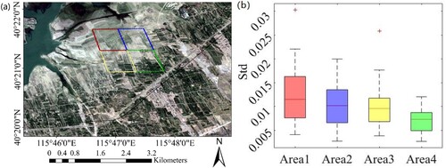
The study was conducted at the Huailai field station, which lies in the semi-arid region of northern China (Hebei Province). There are typical land cover types of Northern China, including cornfields, orchards, woodlands, buildings, and roads. Four 500 m areas featured by different degrees of spatial heterogeneity were selected in order to fully understand the performance of different sampling methods. Here, the degree of spatial heterogeneity was measured by the standard deviations of the high-resolution pixel albedos within the 500 m area. The standard deviation was calculated for each period and its temporal variations indicate the change of spatial heterogeneity within the 500 m area during the experimental period. In this paper, each 500 m sub-region is simulated as a coarse pixel, which refers to the pixel covering a relatively large spatial range and has a significant scale difference with the in situ footprint observation. As shown in Figure 1 (b), Area1 shows the largest spatial heterogeneity and temporal variability. This is because it is close to the Granting reservoir and may be flooded in summer. Area2 and Area3 follow, and Area4 shows the smallest spatial heterogeneity and temporal variability. The different degrees of spatial heterogeneity over these four areas are mainly attributed to different land cover, different farmland management, and different vegetation growth. The divergence of the spatial heterogeneity over these four areas can enhance their representativeness for the general surface condition. Consequently, the conclusions of this study can be more universal.

Figure 1. (a) The map of the study areas and their surroundings. The small colored boxes represent the four 500 m regions with different degrees of spatial heterogeneity. The squares from top to bottom and left to right denote Area1, Area2, Area3, and Area4, respectively. (b) Boxplots of the spatial heterogeneity (denoted as the standard deviation of high-resolution pixel albedo within the 500 m area based on the 33-time albedo images) throughout the year over the four areas.

2.2. High-resolution satellite data

It is important to point out that the optimal sampling was generally carried out prior to in situ measurements, and ancillary data which can reflect the spatiotemporal variation information of surface variables within the coarse pixel were generally utilized as the prior knowledge. In practice, the high-resolution satellite data were often utilized as the prior knowledge to estimate in situ sampling points due to its easy access (Wu et al. 2016, 2021b). It is noteworthy that the definition of high-resolution is not absolute. Instead, it refers to the images which has a much finer resolution than the coarse pixel to be validated. The resolution of the ancillary dataset should, on one hand, enable that the spatial and temporal distribution characteristics of the land surface variables can be captured, and on the other hand, should be close to the footprint of in situ observations.

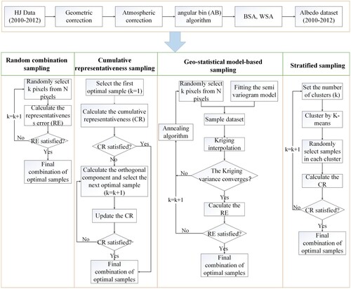
Since the focus of this study aims to evaluate the performance of several recently developed sampling strategies regarding their ability to provide representative in situ albedo observations within the 500 m area, high-resolution ancillary data must be used. Examples of such ancillary datasets could include HuanJing (HJ) CCD images, Landsat TM/OLI images, and Sentinel-2A MSI images which have much finer spatial resolutions than the 500 m. In this study, HJ CCD images were employed partly because of their relatively high update frequency of less than 2 days, and partly because their spatial resolution of 30 m is close to the footprint of in situ albedo measurements as indicated by Wu et al. (2016). The CCD images aboard the HJ satellite from 2010 to 2012 were first atmospherically corrected using the Second Simulation of the Satellite Signal in the Solar Spectrum (6S) radiative transfer code (Kotchenova et al. 2006; Vermote et al. 1997). During this process, the synchronously measured atmosphere parameters were acquired from MODIS aerosol products (at 550 nm). Then they were geo-corrected based on georeferenced Thematic Mapper images. Based on the land surface reflectance dataset, the shortwave black-sky albedo (BSA) and white-sky albedo (WSA) were generated with the angular bin (AB) algorithm (Liang 2003; Qu et al. 2013). By weighting the WSA and BSA with the proportions of diffuse radiation, the blue-sky albedo under the actual atmosphere was generated. The diffuse radiation is a function of the solar zenith angle (SZA) and the atmospheric optical depth (AOD). The AOD information was provided by MODIS aerosol products (at 550 nm). There are 33 albedo maps during the experimental period, which are believed to be able to capture the temporal variations of albedo over the four areas. The high-resolution albedo dataset showed a reasonable accuracy, with a root mean square error (RMSE) of 0.011 and a determination coefficient (R²) of 0.81 over the study area (Wu et al. 2016).

The high-resolution images were used for two purposes in this study. One is to characterize the spatial heterogeneity within the four 500 m areas. The other is to evaluate the performance of different sampling methods by simultaneously simulating the in situ-based measurements and the coarse pixel scale observations. In the latter case, the high-resolution pixel albedo is used to simulate the in situ reporting albedo, and the average of all high-resolution pixel albedos within the 500 m area is used to simulate the true value of coarse pixel scale albedo. Using the same data source can lower the impact of the uncertainties from the high-resolution dataset.

3. Methods

In this study, three recently developed model-based sampling methods, including the cumulative representativeness method (Wu et al. 2016), the geo-statistical model-based sampling method (Wang et al. 2013; Ge et al. 2015), and the random combination method (Wu et al. 2021a) were focused. Since stratified sampling has been widely used over heterogeneous surfaces, its performance was also evaluated and compared to those of three model-based methods. The specific sampling process of the four methods is shown in Figure 2.

Figure 2. The conceptual figure of each sampling method.

3.1. Cumulative representativeness sampling method (CRS)

The basic theory of the cumulative representativeness sampling method is the similarity and orthogonalization between two vectors. The former can enable the representativeness of samples, while the latter can avoid information redundancy and minimize the costs related to the sample size. The first optimal point was selected based on the indicator of representativeness: (1) $r_{i,j}^1={\displaystyle \frac{\left|〈{\alpha }_j\cdot {\text{β}}_i〉\right|}{\sqrt{〈{\alpha }_j\cdot {\alpha }_j〉}\times \sqrt{〈{\text{β}}_j\cdot {\text{β}}_j〉}}}$(1) where ${\alpha }_j$ represents the time sequence albedo vector of HJ pixel $j$ within the 500 m area. ${\text{β}}_i$ represents the HJ pixel albedo time series in which the $ith$ candidate point is located. $r_{i,j}^1$ indicates the representativeness of the $ith$ candidate point to the $jth$ HJ pixel. The overall representativeness of the $ith$ candidate point to the 500 m region is defined as the averaged representativeness of all HJ pixels within the 500 m region: (2) $r_i^1={\displaystyle \frac{1}{N}\sum _{j=1}^N{r}_{i,j}^1}$(2) where $N$ is the number of HJ pixels within the 500 m region. Then the candidate point with the highest representativeness $r_i^1$ is identified as the first optimal sample point.

When selecting more points ($n$ ≥ 2), the information represented by previously selected points has to be excluded by replacing ${\alpha }_j$ with its orthogonal component ${ϵ}^{n-1}\left({\alpha }_j\right)$ with respect to the previously selected $n-1$ optimal points: (3) ${ϵ}^{n-1}\left({\alpha }_j\right)={ϵ}^{n-2}\left({\alpha }_j\right)-{\displaystyle \frac{〈{ϵ}^{n-2}\left({\alpha }_j\right)\cdot {\text{β}}_{n-2}^{\ast }〉}{\begin{array}{c}<{\text{β}}_{n-2}^{\ast }\cdot {\text{β}}_{n-2}^{\ast }\end{array}>}{\text{β}}_{n-2}^{\ast }}$(3) where ${\text{β}}_{n-2}^{\ast }$ is the orthogonal component of the selected $\left(n-1\right)th$ optimal point with respect to the previously selected $n-2$ optimal points. Then the representativeness of candidate point $i$ for pixel $j$ (denoted as $r_{i,j}^n$) can be expressed as: (4) $r_{i,j}^n={\displaystyle \frac{\left|〈{ϵ}^{n-1}\left({\alpha }_j\right)\cdot {\text{β}}_i^{n-1}〉\right|}{\sqrt{〈{ϵ}^{n-1}\left({\alpha }_j\right)\cdot {ϵ}^{n-1}\left({\alpha }_j\right)〉}\times \sqrt{〈{\text{β}}_i^{n-1}\cdot {\text{β}}_i^{n-1}〉}}}$(4) where ${\text{β}}_i^{n-1}$ is the orthogonal component of candidate point $i$ with respect to the previously selected n-1 optimal points.

The cumulative representativeness of these selected points for $jth$ HJ pixel can be defined as: (5) $S{R}_j=\sum _{k=1}^n{r}_{k,j}^k$(5) where $S{R}_j$ denotes the cumulative representation of $jth$ HJ pixel, which ranges from 0 to 1. $k$ denotes the $k$th sampling point.

The cumulative representativeness of these selected points to the 500 m region is defined as the average of the cumulative representativeness of all 30 m pixels within the 500 m area.

3.2. Geo-statistical model-based sampling (GSS)

The geo-statistical model was generally used together with the spatial simulated annealing algorithm to determine the optimal sampling points (Ge et al. 2015). The annealing algorithm is essentially a probability-based algorithm, which reduces the energy and tends to be in order and stable in the process of temperature reduction. The key to this algorithm lies in the selection of initial temperature and end temperature, the construction of objective energy function, as well as the way of adding disturbance and accepting suboptimal solutions. In this study, the initial temperature and the end temperature are set to 1000 and 0.001, respectively. Kriging variance was employed as the target energy function because it is generally utilized to indicate the best sample locations under the condition of unbiased estimation. It is determined by the spatial variation structure and the locations of these samples. It can be expressed by the covariance matrix between the known points and the points to be estimated: (6) ${\delta }^2=C\left(s_0,s_0\right)-C\left(s_0,s_i{)}^{{}^{\mathrm{\prime }}}\right(C\left(s_{\mathrm{i}},s_j\right){)}^{-1}C\left(s_0,s_i\right)+{\displaystyle \frac{{\left(1-I^{\mathrm{\prime }}{\left(C\left(s_{\mathrm{i}},s_j\right)\right)}^{-1}C\left(s_0,s_i\right)\right)}^2}{I^{\mathrm{\prime }}{\left(C\left(s_{\mathrm{i}},s_j\right)\right)}^{-1}I}}$(6) where the covariance function of the sample is represented by $C\left(s_x,s_y\right)$. The $C\left(s_0,s_0\right)$ represents the variance of the point $s_0$ that waiting to be estimated, $C\left(s_{\mathrm{i}},s_j\right)$ indicates the covariance between two known points $s_i$ and $s_j$, $C\left(s_0,s_i\right)$ denotes the covariance between the point to be estimated $s_0$ and known points $s_i$, $I$ is an n-dimensional column vector with all elements of 1. Furtherly, the relationship between covariance and variation function can be expressed as: (7) $\gamma \left(h\right)=C\left(s_0,s_0\right)-C\left(s_0,s_0+h\right)$(7)

As seen from Equations (6) and (7), to obtain the estimated variance of the Kriging equation, it is necessary to know the covariance or variogram of any two points in space, which is usually used to measure the spatial autocorrelation of regionalized variables. Here, the Gaussian model is adopted: (8) $\gamma \left(h\right)=\{\begin{array}{c}0,h=0\\ C_0+C\left(1-e^{{\displaystyle \frac{h^2}{a^2}}}\right),h>0\end{array}$(8) where $C_0$ is the nugget, C is the arch height, h is the distance between two points, which is also known as the lag distance, and the variation range of the Gaussian model is about $\sqrt{3}$a.

When using the annealing algorithm to select samples, we first randomly select a preset number of samples and calculate the initial representativeness error. Then we disturb the locations of these samples randomly and calculate the representative error of the new sample set. The locations of the new sample set will be accepted if the representative error of the new sample set is less than that of the preset sample set (Equation (9)). Otherwise, they will be accepted by a certain probability (Equation (9)) which can enable that the simulated annealing algorithm can escape from the local optimal solution. The disturbance process and the acceptance process will be iterated until the representative error of the selected sample set is small and stable. (9) $p=\{\begin{array}{c}1,E_{t+1}<E_t\\ e^{{\displaystyle \frac{-\left(E_{t+1}-E_t\right)}{KT}}},E_{t+1}\ge E_t\end{array}$(9) where $E_{t+1}$ represents the representative error of the new sample set, $E_t$ refers to the representative error of the preset sample set. K is the cooling coefficient and T is the current temperature.

3.3. Random combination method (RC)

The random combination method has not been widely adopted in the optimal sampling field because of expensive computing costs. Instead, the bootstrap method is generally used to determine the number of required samples (NRS) by fixing replicates. Nevertheless, the fixed repetitions may lead to a local optimal solution and the confidence level fluctuates with sample sizes. Since our original intention is sampling within a coarse pixel, the random combination method which considers all the possible combinations was adopted in this study. Euclidean distance (denoted as Euclidean) was used as the indicator to determine the optimal samples. (10) $Euclidean=\sqrt{{\left(a-b\right)}^2}$(10) where $a$ and $b$ denote the averaged albedo time sequence of the selected pixels and all pixels within the 500 m region, respectively. When we randomly select $K$pixels ($K\le N$) from $N$ available pixels, there will be $C_N^K={\displaystyle \frac{N!}{K!\left(N-K\right)!}\left(K=1,2,3,\dots K\le N\right)}$ possible combinations. For each combination, Equation (10) is calculated. The combination with the minimum Euclidean was identified as the optimal sample. The sampling process comes to end when the minimum Euclidean satisfies the accuracy requirement. Notably, the random combination method mentioned in this paper is essentially a traversal algorithm, which results in a large amount of computation in the case of a large number of samples. In this situation, the top-down multiscale nested sampling method (MNSM) (Wu et al. 2021c), which was established on the random combination method, was employed in this study when the number of samples exceeds 6 in this study.

3.4. Stratified sampling (SS)

Stratified sampling is conducted by dividing the heterogeneous area into several subareas which are more homogeneous, making the variance within the strata smaller than within the whole area. Considering that stratified sampling has many branches, there may be great differences in algorithm performance for different stratified algorithms. In this study, the K-mean clustering was selected to stratify the albedo map of each 500 m area because of its wide acceptance. For each stratum, the samples are randomly selected and then combined to form the final set of sampling results. The core of this algorithm is to iteratively solve the problem of which cluster each object belongs to according to the set number of clustering kernels and loss function. The loss function was defined as the sum of squares of errors between each sample and the center point of the cluster to which it belongs: (11) $J\left(c,\mu \right)=\sum _{i=1}^M|x_i-{\mu }_{c_i}{|}^2$(11) where $x_i$ represents the $i$th sample, $c_i$ is the cluster to which $x_i$ belongs, ${\mu }_{c_i}$ denotes the center point corresponding to the cluster, and M is the total number of samples. Considering that the methods of calculating the average of the stratified samplings may influence the final sampling results, both the arithmetic average (denoted as SSM) and the weighted average (denoted as SSW) method were employed.

3.5. The evaluation method

It is noteworthy that the cost functions of these four sampling methods are different. For the purpose of consistency and comparison, the Representativeness error (denoted as ${ϵ}_{re{p}_{error}}$) of the optimal samples was defined here as the indicator of their performance: (12) ${ϵ}_{re{p}_{error}}=\sqrt{\left(n\ast \sum _{i=1}^n{\left(V_i-{\overline{V}}_i\right)}^2\right)/\sum _{i=1}^n{\overline{V}}_i}\times 100\text{\%}$(12) where $V_i$ represents the mean albedo of the selected samples in time $i$, ${\overline{V}}_i$ denotes the regional mean albedo at the same time, n is the length of time series, and ${ϵ}_{re{p}_{error}}$ represents the mean value of the representativeness error of all images in the whole time series.

In order to fully understand the advantages and disadvantages of these four sampling methods as well as their applicability in different scenarios, they were evaluated from two aspects: one is to compare the minimum number of required samples to meet a predefined Representativeness error (RE) of 3%; the other is to compare their representative errors under each specific number of ground samples.

4. Results and discussion

4.1. The number of required samples within a predefined uncertainty of 3%

The number of required samples (NRS) stands for the minimum number of samples required to estimate the area mean value within a predetermined accuracy (Famiglietti et al. 2008). As shown in Figure 3, the NRS of RC is consistently the smallest among the four methods, which is equal to 3 for Area1 to Area3 and 2 for Area4. CRS follows, with a slightly larger NRS of 5, 6, 5, and 4 for Area1 to Area4, respectively. The NRS of GSS is close to 10 over the four regions. It is noteworthy that the number of required samples by SS shows strong dependence on the methods of calculating the average of the stratified samplings. SSM shows the largest NRS among these four methods except for Area4, where its NRS is equal to CRS but much smaller than GSS. By contrast, SSW consistently requires a smaller NRS than GSS over the four areas.

Figure 3. Histogram of NRS with these sampling methods over the four regions.

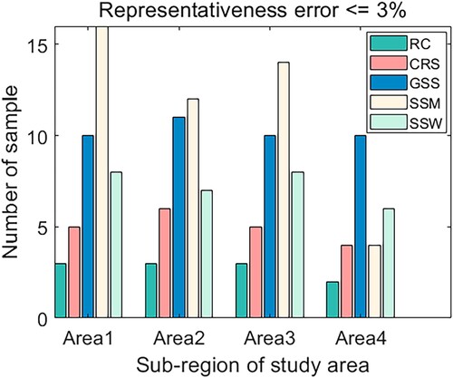
The above results are partly related to the degree of spatial heterogeneity of the 500 m region and partly related to the characteristics of the sampling methods themselves. The best performance of RC can be explained by the fact that it iterates through each possible combination of samples for each specific number of samples to identify the optimal combination with the minimum RE. Hence, the samples in the optimal combination were selected at once and played an equally important role in representing the area mean. Unlike RC, CRS identifies the samples one by one. In fact, the selection of the first optimal sample by CRS is essentially similar to RC. The only difference, however, is that the former stresses the similarity (Equation (1)) while the latter stresses the difference between the sample and the population mean (Equation (10)). When selecting more than 1 sample, the effectiveness of the previously selected nodes has been considered, the orthogonal vectors are decomposed, and the sample which has the most representativeness of the residual information will be selected. The newly selected sample can fill the gap caused by spatial heterogeneity to approximate the area mean. Therefore, the role of the optimal samples by CRS is totally different and more samples are needed to represent the area mean. Regarding the GSS, a relatively larger number of samples are needed to fit the semi-variogram model well, which affects the estimation of Kriging variance. Furthermore, there is a certain randomness in using the spatial simulated annealing algorithm. Its ability to jump out of the locally optimal solution is relatively limited in this situation. The performances of SS show a strong dependence on the methods of calculating the average value. The NRS of SSM is sensitive to the degree of spatial heterogeneity, which is the worst over the area with large spatial heterogeneity (i.e. Area1) and reasonable over the area with small spatial heterogeneity (i.e. Area4). This occurs because the performance of SSM largely depends on the performance of the layered algorithm. Over the seriously heterogeneous surface, sampling on each layer is unfavorable to estimating the area mean, because these layers function unequally to represent the area mean. By contrast, the NRS of SSW seems to be insensitive to spatial heterogeneity, indicated by the similar NRS over the four areas. This is because the weighted average method partially makes up for the effect of spatial heterogeneity. Therefore, SSW should be the first choice when conducting the stratified sampling over heterogeneous surfaces when the NRS is focused.

The abilities of these methods in dealing with spatial heterogeneity also show large difference. The NRS of RC is the smallest over the four sub-areas under a predefined requirement of representativeness error less than 3%. This is related to the fact that its spatial heterogeneity is the smallest among the four areas. By contrast, the NRS of CRS does not necessarily increase with the degree of spatial heterogeneity. For instance, NRS of CRS in Area1 featured by the largest spatial heterogeneity is smaller than that of Area2 with a smaller spatial heterogeneity (Figure 1(b)). The NRS of GSS is always large and almost independent of the degree of spatial heterogeneity within the 500 m region. The NRS of SSM is the most dependent on spatial heterogeneity given the fact that the NRS of Area4 is significantly smaller than that of Area1, but the NRS of SSW does not show obvious dependence on spatial heterogeneity. Based on the above results, it can be concluded that the RC always performs the best for the sampling on the coarse pixel level. CRS is slightly worse than RC. SSM shows the worst performance over the surface with strong heterogeneity but is comparable to CRS when the degree of spatial heterogeneity is not large. The poor performance of SSM in heterogeneous regions can be attributed to the performance of the clustering algorithm. Because samples are randomly selected within the layers, clustering error affects the quality of selected samples. SSW significantly improves the performance of stratified sampling over heterogeneous surfaces, but its superiority disappears over the surfaces with small spatial heterogeneity (i.e. Area4). GSS does not work well on the coarse pixel-level regardless of the degree of spatial heterogeneity.

4.2. The representative errors under each specific number of samples

Figure 4 presents the RE for each specific number of samples with these optimal sampling methods. Since the ultimate aim of sampling is to obtain pixel scale ground observations with negligible RE with a small number of samples, we only present the results for the number of samples ranging from 1 to 6.

Figure 4. The RE of these methods for the number of samples ranging from 1 to 6.

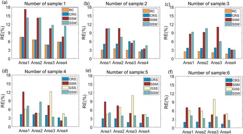
Since the GSS algorithm does not work well with a small number of samples, only the REs of RC, CRS, SSM, and SSW were compared for the number of samples ranging from 1 to 3 (Figure 4(a–c)). When only one sample is available, the REs of RC and CRS are almost the same over Area1 to Area4. The REs of SSM and SSW are always the largest among these methods. Furthermore, the REs of SSM are monotonically decreasing with the degree of spatial heterogeneity (Figure 1(b) and Figure 4(a)). As the number of samples increases to 2, the REs of these three methods consistently decrease except for the CRS increase in Area3 (Figure 4(b)), where the REs of CRS even increased. Moreover, the reduction of RE is more significant for RC, SSM, and SSW than for CRS. It is noteworthy that the RE of RC is close to 3% with 2 samples. With the further increase of sample (Figure 4(c)), REs of RC are consistently smaller than 3% over the four areas. And those of CRS are close to 3%. However, the RE of SS is still very large except for Area4. Furthermore, there is a significant increase of RE of SSM over Area3 when the number of samples increases from 2 to 3. From these results, it can be concluded that increasing the number of samples will not necessarily result in a decrease of overall REs. For instance, increasing the number of samples does not result in a decrease of REs for CRS and SSM over Area3. This phenomenon is determined by the characteristics of their algorithms. The CRS selects the most representative sample for the residual vector after more than one sample was selected, while the effectiveness of SS is related to the stratification error and the mechanism of randomly selecting samples. When only one sample is available, RC and CRS can achieve equally good results. But when more than 1 samples are available, RC shows a distinct advantage over CRS and SS. Although the NRS of SSW is insensitive to the degree of spatial heterogeneity, the REs of SSW show obvious dependence, indicated by the gradual decrease of RE from Area1 to Area4. The performances of SSM over the four regions once again prove that the sampling ability of SSM depends on the degree of spatial heterogeneity. Better results can be achieved in regions with relatively weaker spatial heterogeneity.

Since the REs of RC are very small when the number of samples is equal to 3, they were not discussed with the further increase of samples. From Figure 4(d–f), it can be found that the REs of CRS are significantly smaller than those of SS and GSS, indicating once again that CRS shows an advantage over SS and GSS within the coarse pixel scale. Over Area1 and Area2 where spatial heterogeneity is relatively larger, REs of CRS decrease slightly with the increase of samples. But over Area3 and Area4 where spatial heterogeneity is relatively smaller, there is a very slight gain when the number of samples reaches 5. Regarding the performance of GSS, it is noteworthy that there were no evident changes in REs of GSS with the increase of samples. Though GSS has been widely used and proved to be effective in the watershed scale (Wang et al. 2013; Ge et al. 2015), it does not work very well within a coarse pixel scale. One reason is that the number of samples within the coarse pixel scale is so limited that the basic assumption of GSS cannot be satisfied. Moreover, the REs of GSS seem to be not related to spatial heterogeneity given the fact that Area3 always shows the largest RE among the four areas.

In general, RC shows a distinct advantage over the other three methods within the coarse pixel scale. With the increase of the number of samples, the RE of RC is gradually lowered, which meets the needs of field experiments. The performance of CRS is slightly inferior to RC, but it can also achieve good results over the four areas. However, it is worth noting that the REs of CRS may also increase with the increasing number of samples, because it is based on residual information but not the target variable after more than one sample is selected. SSM does not work well when spatial heterogeneity is large or the number of samples is small. In particular, the performance of SSW is not stable with the number of samples. For instance, SSW even shows larger REs than SSM over Area2 in the case of 3 and 4 samples (Figure 4(c and d)). The performance of GSS is not ideal within the coarse pixel scale, which is mainly due to the limited number of samples.

4.3. The variation pattern of RE with the number of samples

Given the fact that the REs of CRS, SS, and GSS do not change regularly with the number of samples in the case of small sample size (Figure 5), we present their variation pattern by expanding the sample size in order to have a general understanding of the variation of RE with the increase of ground samples. As shown in Figure 5(a–d), the RE of RC first decreases monotonically with the number of samples when the number of samples is less than and equal to 3. However, with the further increase of samples, there is a small fluctuation of RE in a certainty scope. This indicates that in the case of optimal sampling, there is an optimal (minimum) number of samples with which the requirement of RE can be satisfied. No more gains can be achieved with the further increase of samples. Moreover, it is noteworthy that the RE of RC is the smallest among these four methods when the number of samples is less than and equal to 4. The minimum RE of 2% can be achieved with 4 samples over Area1 and Area2. For Area3 and Area4, the minimum RE is even smaller than 2% with the optimal number of 3 samples. This shows once again the distinct advantage of RC in the optimal sampling within the coarse pixel scale. Despite the fluctuation of its RE with the further increase of samples, it is still the minimum or near to minimum.

Figure 5. The variation of RE with the number of samples over the four areas.

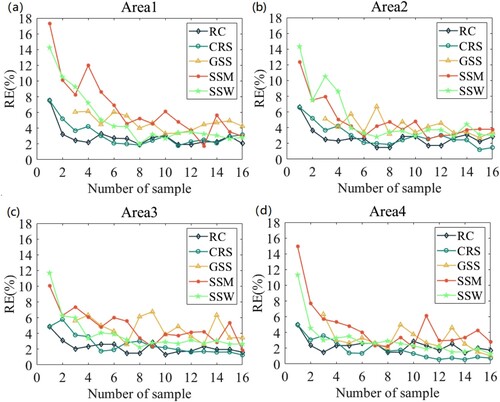
The REs of CRS basically present a downward trend over the four areas when the number of samples is less than or equal to 6. After that, the RE is relatively stable, indicating low gain beyond. It is noteworthy that although the RE of CRS presents a clear decreasing trend when the number of samples is less than and equal to 3, its decreasing rate is much smaller than that of RC, indicating that the RE is more sensitive to the number of samples in RC than CRS. Hence, the CRS is not as good as RC in the case of small samples. Another noteworthy phenomenon is that the RE of CRS is the smallest among these four methods when the number of samples is larger than and equal to 10 over Area4. The minimum RE is even close to 0 when the number of samples reaches 12. But this does not occur in the other three areas. This result indicates that over the surface with relatively small spatial heterogeneity, the RE of in situ measurements close to 0 can be achieved at the expense of a large number of samples. In this situation, the CRS is more effective than RC. This occurs because the samples selected later represent residual information that cannot be represented by previously selected samples. Nevertheless, over the area with relatively large spatial heterogeneity (i.e. Area1 and Area2), there is no clear difference between RC and CRS regarding their ability to reduce RE when the number of samples is larger than and equal to 6. The RE close to 0 cannot be achieved with the limited number of samples by these two methods (Figure 5(a–b)).

The RE of GSS does not show a decreasing trend with the increase of samples (Figure 5). Instead, RE shows relatively large fluctuations ranging from 3% to 6%. This demonstrates that increasing the number of samples does not bring about obvious benefits. The slight fluctuation can be partly attributed to the limited ability of GSS to jump out of the local optimal solution and partly attributed to the fact that the Kriging variance of the samples cannot represent that of the whole area. This result proves once again that the effectiveness of GSS decreases within the coarse pixel scale, despite their wide acceptance on the watershed scale. This is mainly caused by the fact that the semi-variogram model has limited expression of spatial autocorrelation properties in the region, and the regionalized variables of albedo in the region may not adapted to the second-order stationary hypothesis.

Over the four areas, as the number of samples increases from 1 to 6, there was a dramatic decrease in RE of SSM, with values from more than 10% to about 5% (Figure 5(a–d)). Moreover, it is obvious that the RE of SSM is always the largest among these four methods when the number of samples is less than 4, with an exception over Area4 when the number of samples is 3. This result demonstrates that SSM is not a good choice when only a small number of samples are available. With the further increase of samples, the RE of SSM fluctuates widely from 2% to 6%. The RE of SSM is basically comparable to that of GSS. Nevertheless, it is noteworthy that SSM presents the smallest RE among these four methods with 13 samples over Area1 (Figure 5(a)). A similar phenomenon can be found in Area3 with 9 samples and Area4 with 7 samples. Hence, it can be concluded that in the case of a relatively large number of samples available (>=7), the performance of SSM is jointly influenced by spatial heterogeneity and the number of samples. The RE variation trend of SSW is similar to SSM in the case of small samples (<=6). Nevertheless, when the number of samples exceeds 6, SSW is almost unchanged with the increase of samples. It is noteworthy that there are intersection points on the REs of SSM and SSW in Area1, Area2, and Area3 in the case of small samples. Hence, the superiority of SSW is not absolute.

In summary, REs of RC and CRS are consistently smaller than those of GSS and SS, indicating the better performance of the former within the coarse pixel scale. Moreover, the fluctuation ranges of REs of RC, SSW, and CRS are smaller than those of GSS and SSM, indicating the robustness and stability of these algorithms. Particularly, RC shows a distinct advantage over CRS in the case of small samples. Nevertheless, when the goal of sampling is to obtain in situ measurements with RE close to 0 at the expense of a large number of samples, CRS is more effective than RC in areas with relatively small spatial heterogeneity. Nevertheless, over the area with relatively large spatial heterogeneity, the performance of RC and CRS is comparable, and the goal of RE close to 0 cannot be achieved with the limited number of samples. The performance of GSS is unexpected partly because of its relatively larger RE and partly because the RE of GSS seems to be independent of the number of samples. The fundamental cause of this phenomenon is that the number of samples within the coarse pixel scale cannot support the characterization of the spatial autocorrelation characteristics of surface albedo within the coarse pixel, reducing the effectiveness of GSS. SS is not suggested within the coarse pixel in the case of only a small number of samples available. But when more samples are available, the effectiveness of SS shows a strong dependence on the spatial heterogeneity, the number of samples, and the methods of calculating average value. The REs of SSW are generally smaller and more stable than those of SSM. It is important to note that in the case of optimal sampling, the RE of samples is related to the number of samples. But the increase of samples does not necessarily result in a decreased RE. Hence, the optimal number of samples which provides the best tradeoff between RE and the field observe cost should be adopted.

5. Conclusion

Ground optimal sampling is an essential part of validation due to the large spatial scale mismatch between in situ and satellite-measurements as well as the spatial heterogeneity. Although various sampling approaches have been proposed, their effectiveness within the coarse pixel scale have not been fully understood. Given that their ability to address spatial heterogeneity is different and that the assumptions may be difficult to be satisfied within the coarse pixel, this study conducted the first assessment of four recently developed sampling methods regarding their ability to provide representative observations within the coarse pixel scale.

Four 500 m areas with different degrees of spatial heterogeneity were selected in order to facilitate the generalization of the conclusions. It was found that RC generally shows the best performance among these methods, with the least number of samples to satisfy the predefined uncertainty of 3%. Moreover, its REs are always the smallest among these methods in the case of a small number of samples. Therefore, it should be the first choice for ground sampling within a coarse pixel. However, when the goal of sampling is to obtain in situ measurements with RE close to 0 at the expense of a large number of samples, CRS is more effective than RC in areas with relatively small spatial heterogeneity. Nevertheless, over the area with relatively large spatial heterogeneity, the performance of RC and CRS is comparable, and the goal of RE close to 0 cannot be achieved with the limited number of samples.

Despite the wide acceptance of GSS on the watershed scale, the effectiveness of GSS decreases within the coarse pixel scale, partly because the number of samples cannot support a robust and representative semi-variogram model, and partly because of the limitations of the spatial simulated annealing algorithm. In fact, the GSS algorithm tends to be stable only when more than 20 samples are available. Therefore, this method is not the best choice for sampling on the coarse pixel level. SSM is not suggested within the coarse pixel in the case of only a small number of samples available, because it always presents the largest RE among these methods. It is important to note that although the SSW outperforms SSM over heterogeneous surfaces when the NRS was focused, its superiority is not absolute because there are intersection points on the REs of SSM and SSW. In fact, the hierarchical algorithms in SSM have many branches. Better results may be achieved when taking different hierarchical clustering algorithms or giving weights to samples (e.g. SSW in this paper), or combining them with intelligent optimization algorithms like the Latin hypercube method.

It is important to note that in the case of optimal sampling, the RE of samples is related to the number of samples. But the increase of samples does not necessarily result in a decreased RE. Hence, the optimal number of samples which provides the best tradeoff between RE and the field observation cost should be adopted. The next important thing to notice is that the conclusion of this study is only applicable to the sampling within the coarse pixel. In fact, different methods have different application scenarios. Hence, the effectiveness of the sampling methods should be evaluated for different purposes and applications. The last and most important thing to notice is that the findings and conclusions of this study are based on the 30 m HJ albedo data over a small area which is not representative of general conditions of natural surfaces. Therefore, it is an open issue whether the findings and conclusions still hold when a much finer spatial resolution ancillary dataset (e.g. the observations made by unmanned aerial vehicle) is used and whether the conclusions are applicable to other areas or other surface variables (e.g. leaf area index and soil moisture). Although it is only a case study, the results presented provide a useful insight into the characteristics of different sampling methods, which give important guidance for the sampling deployment and new perspectives for the uncertainty of ground albedo ‘truth’ on the coarse pixel scale.

Disclosure statement

No potential conflict of interest was reported by the author(s).

Data availability statement

The digital products of HuanJing (HJ) satellite are publicly available at http://www.secmep.cn/sjcp/sjcpzs/201703/t20170324_563108.shtml, and the MODIS aerosol products (at 550 nm) can get at https://ladsweb.modaps.eosdis.nasa.gov/search/.

Additional information

Funding

This work was supported by the National Natural Science Foundation of China [grant number 42071296], the China High-Resolution Earth Observation System [grant number 21-Y20B01-9001-19/22], and the Fundamental Research Funds for the Central Universities [grant number lzujbky-2022-09].

References

- Boschetti, L., S. V. Stehman, and D. P. Roy. 2016. “A Stratified Random Sampling Design in Space and Time for Regional to Global Scale Burned Area Product Validation.” Remote Sensing of Environment 186: 465–478. doi:10.1016/j.rse.2016.09.016.
- Cochran, W. 1977. Sampling Techniques. New York: Wiley.
- Famiglietti, J. S., D. Ryu, A. A. Berg, M. Rodell, and T. J. Jackson. 2008. “Field Observations of Soil Moisture Variability Across Scales.” Water Resources Research 44 (1). doi:10.1029/2006WR005804.
- Ge, Y., J. H. Wang, G. B. Heuvelink, R. Jin, X. Li, and J. F. Wang. 2015. “Sampling Design Optimization of a Wireless Sensor Network for Monitoring Ecohydrological Processes in the Babao River Basin, China.” International Journal of Geographical Information Science 29 (1): 92–110. doi:10.1080/13658816.2014.948446.
- Hitchcock, D. B. 2003. “A History of the Metropolis–Hastings Algorithm.” The American Statistician 57 (4): 254–257. doi:10.1198/0003130032413.
- Kotchenova, S. Y., E. F. Vermote, R. Matarrese, and F. J. Klemm. 2006. “Validation of a Vector Version of the 6S Radiative Transfer Code for Atmospheric Correction of Satellite Data Part I: Path Radiance.” Applied Optics 45 (26): 6762–6774. doi:10.1364/AO.45.006762.
- Liang, S. 2003. “A Direct Algorithm for Estimating Land Surface Broadband Albedos From MODIS Imagery.” IEEE Transactions on Geoscience and Remote Sensing 41 (1): 136–145. doi:10.1109/TGRS.2002.807751.
- Minasny, B., and A. B. McBratney. 2006. “A Conditioned Latin Hypercube Method for Sampling in the Presence of Ancillary Information.” Computers and Geosciences 32 (9): 1378–1388. doi:10.1016/j.cageo.2005.12.009.
- Morisette, J. T., F. Baret, J. L. Privette, R. B. Myneni, J. E. Nickeson, S. Garrigues, and R. Cook. 2006. “Validation of Global Moderate-Resolution LAI Products: A Framework Proposed Within the CEOS Land Product Validation Subgroup.” IEEE Transactions on Geoscience and Remote Sensing 44 (7): 1804–1817. doi:10.1109/TGRS.2006.872529.
- Mu, X., M. Hu, W. Song, G. Ruan, Y. Ge, J. Wang, and G. Yan. 2015. “Evaluation of Sampling Methods for Validation of Remotely Sensed Fractional Vegetation Cover.” Remote Sensing 7 (12): 16164–16182. doi:10.3390/rs71215817.
- Peng, J., Q. Liu, J. Wen, Q. Liu, Y. Tang, L. Wang, and J. Shi. 2015. “Multi-Scale Validation Strategy for Satellite Albedo Products and its Uncertainty Analysis.” Science China Earth Sciences 58 (4): 573–588. doi:10.1007/s11430-014-4997-y.
- Qu, Y., Q. Liu, S. Liang, L. Wang, N. Liu, and S. Liu. 2013. “Direct-Estimation Algorithm for Mapping Daily Land-Surface Broadband Albedo From MODIS Data.” IEEE Transactions on Geoscience and Remote Sensing 52 (2): 907–919. doi:10.1109/TGRS.2013.2245670.
- Vermote, E. F., N. El Saleous, C. O. Justice, Y. J. Kaufman, J. L. Privette, L. Remer, and D. Tanre. 1997. “Atmospheric Correction of Visible to Middle-Infrared EOS-MODIS Data Over Land Surfaces: Background, Operational Algorithm and Validation.” Journal of Geophysical Research: Atmospheres 102 (D14): 17131–17141. doi:10.1029/97JD00201.
- Walvoort, D. J., D. J. Brus, and J. J. De Gruijter. 2010. “An R Package for Spatial Coverage Sampling and Random Sampling From Compact Geographical Strata by k-Means.” Computers and Geosciences 36 (10): 1261–1267. doi:10.1016/j.cageo.2010.04.005.
- Wang, J., Y. Ge, G. B. Heuvelink, and C. Zhou. 2013. “Spatial Sampling Design for Estimating Regional GPP with Spatial Heterogeneities.” IEEE Geoscience and Remote Sensing Letters 11 (2): 539–543. doi:10.1109/LGRS.2013.2274453.
- Wen, J., X. Wu, J. Wang, R. Tang, D. Ma, Q. Zeng, and Q. Xiao. 2022. “Characterizing the Effect of Spatial Heterogeneity and the Deployment of Sampled Plots on the Uncertainty of Ground “Truth” on a Coarse Grid Scale: Case Study for Near-Infrared (NIR) Surface Reflectance.” Journal of Geophysical Research: Atmospheres 127 (11): e2022JD036779. doi:10.1029/2022JD036779.
- Wu, X., J. Wen, Q. Xiao, Y. Bao, D. You, J. Wang, and B. Gong. 2021a. “Quantification of the Uncertainty Caused by Geometric Registration Errors in Multiscale Validation of Satellite Products.” IEEE Geoscience and Remote Sensing Letters 19: 1–5. doi:10.1109/LGRS.2021.3099833.
- Wu, X., J. Wen, Q. Xiao, Q. Liu, J. Peng, B. Dou, and Q. Liu. 2016. “Coarse Scale in Situ Albedo Observations Over Heterogeneous Snow-Free Land Surfaces and Validation Strategy: A Case of MODIS Albedo Products Preliminary Validation Over Northern China.” Remote Sensing of Environment 184: 25–39. doi:10.1016/j.rse.2016.06.013.
- Wu, X., J. Wen, Q. Xiao, D. You, B. Gong, J. Wang, and X. Lin. 2021b. “Spatial Heterogeneity of Albedo at Subpixel Satellite Scales and its Effect in Validation: Airborne Remote Sensing Results From HiWATER.” IEEE Transactions on Geoscience and Remote Sensing 60: 1–14. doi:10.1109/TGRS.2021.3124026.
- Wu, X., J. Wen, Q. Xiao, D. You, X. Lin, S. Wu, and S. Zhong. 2019b. “Impacts and Contributors of Representativeness Errors of In Situ Albedo Measurements for the Validation of Remote Sensing Products.” IEEE Transactions on Geoscience and Remote Sensing 57 (12): 9740–9755. doi:10.1109/TGRS.2019.2928954.
- Wu, X., J. Wen, Q. Xiao, D. You, J. Wang, D. Ma, and X. Lin. 2021c. “A Multiscale Nested Sampling Method for Representative Albedo Observations at Various Pixel Scales.” IEEE Journal of Selected Topics in Applied Earth Observations and Remote Sensing 14: 8193–8207. doi:10.1109/JSTARS.2021.3105562.
- Wu, X., Q. Xiao, J. Wen, D. You, and A. Hueni. 2019a. “Advances in Quantitative Remote Sensing Product Validation: Overview and Current Status.” Earth-Science Reviews 196: 102875. doi:10.1016/j.earscirev.2019.102875.
- Xie, H., X. Tong, W. Meng, D. Liang, Z. Wang, and W. Shi. 2015. “A Multilevel Stratified Spatial Sampling Approach for the Quality Assessment of Remote-Sensing-Derived Products.” IEEE Journal of Selected Topics in Applied Earth Observations and Remote Sensing 8 (10): 4699–4713. doi:10.1109/JSTARS.2015.2437371.
- Xie, H., F. Wang, Y. Gong, X. Tong, Y. Jin, A. Zhao, and S. Liao. 2022. “Spatially Balanced Sampling for Validation of GlobeLand30 Using Landscape Pattern-Based Inclusion Probability.” Sustainability 14 (5): 2479. doi:10.3390/su14052479.
- Zhang, R., J. Tian, Z. Li, H. Su, S. Chen, and X. Tang. 2010. “Principles and Methods for the Validation of Quantitative Remote Sensing Products.” Science China Earth Sciences 53 (5): 741–751. doi:10.1007/s11430-010-0021-3.
- Zhang, M., C. Wang, J. Bu, L. Li, and Z. Yu. 2017. “An Optimal Sampling Method for Web Accessibility Quantitative Metric and its Online Extension.” Internet Research 27 (5): 1190–1208. doi:10.1145/2745555.2746663.
- Zhao, X., J. Liang, and C. Dang. 2019. “A Stratified Sampling Based Clustering Algorithm for Large-Scale Data.” Knowledge-Based Systems 163: 416–428. doi:10.1016/j.knosys.2018.09.007.