Assessing OSM building completeness for almost 13,000 cities globally

ABSTRACT

OpenStreetMap (OSM) is an essential source for acquiring building data, although such data may suffer from quality issues. Many studies have focused on assessing OSM building data quality but few have been carried out on a global scale. This study aims to assess OSM building completeness (a quality measure) for 12,975 cities across the globe. This was achieved by employing population grid data as a proxy for reference building data. Not only the completeness of each city but also that of the grids within that city was assessed. The assessment results were evaluated based on calculating the overall accuracy and the r-square value between estimated and reference OSM building completeness values. Results showed that for 75% of cities, the completeness is lower than 20%; no more than 9% of cities have an estimated completeness higher than 80%. The overall accuracies of most countries were higher than 80%. The estimated completeness was also highly correlated with the reference completeness, which verifies the effectiveness of our approach. These results may be useful for acquiring and updating building data in OSM. A global and open dataset related to OSM building completeness has been made available for public use.

KEYWORDS:

• OpenStreetMap
• building data
• data quality
• population data
• WorldPop

1. Introduction

Building (footprints) data represent the perimeter outline of each building, and they have been viewed as an essential data source for planners and designers to understand our built-up environments. Specific applications may include predicting urban building energy use (Reinhart and Davila 2016; Hong et al. 2020; Wang et al. 2021; Wang et al. 2022), estimating population distribution (Huang et al. 2021; Boo et al. 2022; Qiu et al. 2022), creating three-dimensional (3D) city modeling (Bagheri, Schmitt, and Zhu 2019; Park and Guldmann 2019) and producing land use maps (Li et al. 2021). Thus, it is necessary to acquire building data (especially in a city) to support various applications.

Remote sensing has been widely used to acquire building data. Numerous studies have used deep-learning networks for automatic building extraction from high-resolution remote-sensing images (Xu et al. 2018; Li et al. 2019; Shao et al. 2020). A study has also proposed a semisupervised method for updating existing building data from bitemporal remote-sensing images (Guo et al. 2021). Nevertheless, very high-resolution remote-sensing data (e.g. less than 1-m resolution) are still not freely available for most countries and regions. Moreover, there may be technical challenges for most planners and designers to use remote-sensing data because a series of processing steps (including image calibration, segmentation, and/or classification, detection and/or identification) are often needed. As an alternative, the geospatial data provided by global volunteers (known as volunteered geographic information or VGI, Goodchild 2007) have also been used for acquiring building data. OpenStreetMap (OSM) is such a VGI platform (https://www.openstreetmap.org/). In OSM, there are multiple types of geospatial data (e.g. roads, buildings, railways, rivers, and land uses), which have been provided by more than eight million volunteers globally [https://wiki.openstreetmap.org/wiki/Stats#Nodes.2C_ways_and_relations, accessed on Jan 2022] and, thus, the data have been viewed as an essential component of Digital Earth (Mooney and Corcoran 2014). There are several benefits of using OSM data. First of all, the data are freely acquirable. Second, the data are being updated on a minute-by-minute basis and, thus, it is possible to acquire building data of the highest recency. Third, the data are in vector format and they can be directly acquired from this platform, which means the data are acquirable with fewer technical challenges. Despite these advantages, concerns have arisen about OSM data quality. Several studies have reported that OSM data quality may vary with different countries and regions (Tian, Zhou, and Fu 2019; Zhou, Wang, and Liu 2022). Therefore, it is necessary to assess data quality before using the OSM data.

Extensive studies have focused on assessing OSM data quality from different quality measures, e.g. positional accuracy (Haklay 2010; Helbich et al. 2012; Fan et al. 2014; Brovelli and Zamboni 2018; Zhou and Jing 2022), attribute accuracy (Girres and Touya 2010; Dorn, Törnros, and Zipf 2015), and completeness (Zhou 2018; Tian, Zhou, and Fu 2019; Wang, Zhou, and Tian 2020; Zhang et al. 2022). The completeness, a measure of how well a region has been mapped, is viewed as the most important quality measure because the other measures are assessed based on existing OSM data. Most studies have assessed OSM data quality by comparing with a reference dataset (e.g. acquired from either a mapping agency or a commercial company). For instance, Fan et al. (2014) assessed the OSM building data quality for Munich, Germany, in terms of various quality measures (e.g. completeness, semantic accuracy, positional accuracy, and shape accuracy) by using building data in the German Authoritative Topographic – Cartographic Information System (ATKIS) as reference data. Brovelli and Zamboni (2018) provided a map-matching method to check both the completeness and spatial accuracy of OSM building data, based on a comparison with the Regional Topographical Geodatabase of Italy. Törnros et al. (2015) compared two completeness measures, i.e. a count ratio (number of OSM buildings divided by the number of reference buildings) and an area ratio (total OSM building area divided by the total reference building area). They concluded that the count ratio underestimates the completeness within a study area and the area ratio overestimates the completeness.

However, the above studies have only investigated OSM building completeness for a few countries and regions. This is because a reference building dataset may not always be freely available. Thus, some studies have proposed the use of proxy indicators to estimate OSM building data quality (called an intrinsic approach; Barron, Neis, and Zipf 2014; Senaratne et al. 2017). Zhou (2018) proposed a building density indicator as a proxy to quantitatively estimate the completeness of OSM building data. Tian, Zhou, and Fu (2019) employed two quality indicators, i.e. OSM building count and OSM building density, to explore the temporal and spatial patterns of OSM building data in China. They concluded that the OSM building data in China are far from being complete. But, as discussed by Zhou (2018), the building density may vary in different geographical regions and the quantitative relationship obtained from analyzing one study area may not always be applicable to others. Recently, Zhang et al. (2022) proposed the use of global open and high-resolution population data as a proxy for reference building data to assess the OSM building data completeness. The tenet of this approach is to assume that there are populations living in the regions with buildings. Based on this assumption, Zhang et al. (2022) used a high-resolution (e.g. 100-m) population grid as the basic unit to determine whether there is a building in each grid (called grid-based assessment). With this approach, there is no need to use reference building data. Thus, this approach may be used for a potential global study. However, in the study of Zhang et al. (2022), only four study areas were involved in the validation. It is therefore necessary to investigate the following:

• How to assess OSM building completeness on a city-wide basis rather than on a grid basis;

• whether the approach can be used for assessing OSM building completeness for cities globally; and

• what the spatial pattern is for OSM building completeness in global cities.

To fill these gaps, this study assesses OSM building completeness for almost 13,000 cities globally. To the best of our knowledge, this is the first time that such a large number of samples have been involved in analysis. Moreover, we proposed an approach to quantitatively estimate OSM building completeness for each city, which can be viewed as an extension of the approach proposed by Zhang et al. (2022). Our results showed that a high overall accuracy (e.g. 80%) and a high consistency (e.g. the r-square value is approximately 0.99) between the estimated and reference OSM building completeness can be achieved by applying this approach to different countries and regions.

This work is structured as follows: Section 2 introduces the approaches for assessing OSM building completeness in each city and also the methods for evaluating the proposed approaches. Section 3 describes the experimental data and steps. Section 4 reports the experimental results and analyses. Section 5 and 6 are the discussions and conclusion, respectively.

2. Methodology

2.1. Assessment approaches

We employed the approach proposed by Zhang et al. (2022). The tenet of this approach is to use a high-resolution population grid as a proxy for reference building data, which is then compared with OSM building data. With this grid-based approach, it is possible to determine whether a grid cell (e.g. 100 m) has been mapped with OSM building data. Based on this approach, we also propose to quantitatively assess the completeness of each city, which is called a city-based assessment.

1. Grid-based assessment

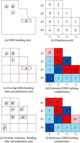
To illustrate the approach of Zhang et al. (2022), a group of schematic maps are produced (Figure 1). Specifically, this figure shows OSM building data with four buildings (Figure 1a) and a population grid with 13 cells (Figure 1b). Each grid cell was qualitatively analyzed using the grid-based assessment. Each of these grid cells has a population count, which varies from 0 (e.g. R1C1) to 5 (e.g. R3C3). According to the assumption that there is a building in which people live (Zhang et al. 2022), we can overlap the OSM building data and the population grid (Figure 1c), and classify each grid cell into one of the following four types (Figure 1d).

• Type I (No-building and No-population): there is no OSM building and the population count is equal to 0 (e.g. R2C1, R3C1, R4C2, R4C3, and R4C4);

• Type II (No-building and With-population): there is no OSM building but the population count is larger than 0 (e.g. R2C3, R3C2, and R4C1);

• Type III (With-building and No-population): there is at least one OSM building but the population count is equal to 0 (e.g. R1C1); or

• Type IV (With-building and With-population): there is at least one OSM building and the population count is larger than 0 (e.g. R1C2, R2C2, R3C3, and R3C4).

  Figure 1. Illustrating the assessment (a, b, c, and d) and evaluation (e and f) approaches with schematic maps.

  

(2) City-based assessment

Next, to quantitatively assess the OSM building completeness of each city, a city-based assessment was also proposed in our study. The principle of the city-based assessment is to calculate the ratio of grid cells with OSM building data proportional to those with estimated building data. That is, (1) $C_{estimated}={\displaystyle \frac{N_{Type\mathrm{I}\mathrm{I}\mathrm{I}}+N_{Type\mathrm{I}\mathrm{V}}}{N_{Type\mathrm{I}\mathrm{I}}+N_{Type\mathrm{I}\mathrm{I}\mathrm{I}}+N_{Type\mathrm{I}\mathrm{V}}}\times 100\text{\%}}$(1) where, $C_{estimated}$ denotes the estimated OSM building completeness of a city. $N_{Type\mathrm{I}\mathrm{I}}$, $N_{Type\mathrm{I}\mathrm{I}\mathrm{I}}$, and $N_{Type\mathrm{I}\mathrm{V}}$ denote the number of grid cells that are classified as Type II, Type III, and Type IV, respectively. According to the definitions of the four types above, there is probably a lack of OSM building data only for Type II. On the contrary, there are OSM building data for Types III and IV. Moreover, the $C_{estimated}$ value varies from 0 to 1. 0 means there are not any OSM building data in a city, and 1 means there is no grid cell that has been classified as Type II.

2.2. Evaluation methods

To evaluate the effectiveness of the two assessment approaches, reference building data are needed. The tenet of this evaluation is to compare between estimated OSM building completeness (based on population grid data) and reference OSM building completeness. Specifically, grid-based evaluation and city-based evaluation were used.

1. Grid-based evaluation

The reference building completeness was assessed for each grid cell to evaluate the effectiveness of the grid-based assessment. To be specific, reference building data (e.g. a total of seven reference buildings in Figure 1e) are first overlapped with the OSM building data and the population grid data, and then each grid cell can be classified as one of the following four types (Figure 1f). That is,

• Type I′: there is no OSM building and no reference building (e.g. R2C1, R3C1, R4C2, R4C3, and R4C4);

• Type II′: there is no OSM building but there is at least one reference building (e.g. R2C3, R3C2, and R4C1);

• Type III′: there is at least one OSM building but there is no reference building (e.g. R3C4); or

• Type IV′: there is at least one OSM building and one reference building (e.g. R1C1, R1C2, R2C2, and R3C3).

Moreover, the four types (I′, II′, III′, and IV′) determined using reference building data can be compared with those types (I, II, III, and IV) determined using population grid data. A confusion matrix was employed for the quantitative evaluation (Table 1), and the following nine measures were calculated. (2) $P{A}_{{\mathrm{I}}^{\mathrm{\prime }}}={\displaystyle \frac{N_1}{N_1+N_3}\times 100\text{\%}}$(2) (3) $U{A}_{\mathrm{I}}={\displaystyle \frac{N_1}{N_1+N_2}\times 100\text{\%}}$(3) (4) $P{A}_{\mathrm{I}{\mathrm{I}}^{\mathrm{\prime }}}={\displaystyle \frac{N_4}{N_2+N_4}\times 100\text{\%}}$(4) (5) $U{A}_{\mathrm{I}\mathrm{I}}={\displaystyle \frac{N_4}{N_3+N_4}\times 100\text{\%}}$(5) (6) $P{A}_{\mathrm{I}\mathrm{I}{\mathrm{I}}^{\mathrm{\prime }}}={\displaystyle \frac{N_5}{N_5+N_7}\times 100\text{\%}}$(6) (7) $U{A}_{\mathrm{I}\mathrm{I}\mathrm{I}}={\displaystyle \frac{N_5}{N_5+N_6}\times 100\text{\%}}$(7) (8) $P{A}_{\mathrm{I}{\mathrm{V}}^{\mathrm{\prime }}}={\displaystyle \frac{N_8}{N_6+N_8}\times 100\text{\%}}$(8) (9) $U{A}_{\mathrm{I}\mathrm{V}}={\displaystyle \frac{N_8}{N_7+N_8}\times 100\text{\%}}$(9) (10) $OA={\displaystyle \frac{N_1+N_4+N_5+N_8}{N_1+N_2+N_3+N_4+N_5+N_6+N_7+N_8}\times 100\text{\%}}$(10)

• (2) City-based evaluation

  Table 1. The confusion matrix for comparing between estimated and reference OSM building completeness*.

  Type	I'	II'	III'	IV'	UA
  I	N1	N2	–	–	UAI
  II	N3	N4	–	–	UAII
  III	–	–	N5	N6	UAIII
  IV	–	–	N7	N8	UAIV
  PA	PAI′	PAII′	PAIII′	PAIV'	OA

  *Note: N denotes the number of grid cells; UA denotes user accuracy; PA denotes producer accuracy; OA denotes overall accuracy.

To evaluate the effectiveness of the city-based assessment, the reference OSM building completeness was also assessed for each city. That is, (11) $C_{reference}={\displaystyle \frac{N_{Type{\mathrm{I}\mathrm{I}\mathrm{I}}^{\mathrm{\prime }}}+N_{Type\mathrm{I}{\mathrm{V}}^{\mathrm{\prime }}}}{N_{Type\mathrm{I}{\mathrm{I}}^{\mathrm{\prime }}}+N_{Type\mathrm{I}\mathrm{I}{\mathrm{I}}^{\mathrm{\prime }}}+N_{Type{\mathrm{I}\mathrm{V}}^{\mathrm{\prime }}}}}$(11) where, $C_{reference}$ denotes the reference OSM building completeness of a city. $N_{Type\mathrm{I}{\mathrm{I}}^{\mathrm{\prime }}}$ $N_{Type\mathrm{I}\mathrm{I}{\mathrm{I}}^{\mathrm{\prime }}}$, and $N_{Type\mathrm{I}{\mathrm{V}}^{\mathrm{\prime }}}$ denote the number of grid cells that are classified as Type II′, Type $\mathrm{I}\mathrm{I}{\mathrm{I}}^{\mathrm{\prime }}$ and Type IV′, respectively. The $C_{reference}$ value also varies from 0 to 1.

Furthermore, not only the linear relationship between the estimated and reference OSM building completeness was plotted, but also the r-square (R²) was used to quantitatively analyze the consistency between these two measures ($C_{estimated}$ and $C_{reference}$). Specifically, (12) $R^2=1-{\displaystyle \frac{\sum {(C_{reference}-C_{estimated})}^2}{\sum {\left(C_{reference}-\overline{C_{reference}}\right)}^2}}$(12) where, $\overline{C_{reference}}$ denotes the average of the reference OSM building completeness for cities.

For the two evaluation methods, it may also be possible to visually determine the type of each grid cell by referring to Google Earth images, especially when reference building data are not available.

3. Data

3.1. Experimental data

The purpose of our study is to assess OSM building completeness for cities globally. Four categories of data were involved in the analysis.

• 1) OSM building data: the OSM data were downloaded from a third-party platform (http://download.geofabrik.de/index.html) in January 2020. This platform has provided OSM data for almost all countries and regions worldwide. The OSM data were saved in shapefile format, which can be easily processed and analyzed by most geographic information system software (e.g. ArcGIS and QGIS). In this platform, the OSM data has been organized into several geographical features or layers, e.g. buildings, roads, land use, water, and railways. Only the buildings layer is acquired for the analysis.

• 2) Reference building: The reference building data of eight different countries (England, France, New Zealand, Australia, United States, Canada, Uganda, and Tanzania) were acquired from different data soeen set correctlurces for the analysis (Table 2). Specifically, the reference building data for England was produced by the Ordnance Survey (the mapping agency of the United Kingdom) and presented at a scale of 1:10,000¹; that for New Zealand was acquired from the Land Information of New Zealand, and presented at a scale of 1:50,000 and with a minimum building size of 10 square meters²; and that for France was acquired from the National Institute of Geographic and Forestry Information (France), and presented at a scale of 1:25,000 and with a minimum building size of 20 square meters³. The building data for the other five countries (Australia, United States, Canada, Uganda, and Tanzania) were produced by the Microsoft company. An existing study (Heris et al. 2020) has reported that the completeness of the Microsoft building data is higher than 93% for buildings larger than 200 m². These building data were involved in the analysis not only because they can be used as references for evaluating our estimated results, but also because they are freely acquirable. In contrast, such reference building data are still not available for most countries and regions in the world.

• 3) Population grid data: A global open and high-resolution population grid dataset (WorldPop, https://www.worldpop.org/) was acquired for the analysis (Bondarenko et al. 2020). The acquired dataset employs random forests to disaggregate census data to high-resolution grid cells that contain built settlements (Stevens et al. 2015; Reed et al. 2018). There are several advantages of using the WorldPop population data. First, the data cover 95% of the countries in the world. Second, the data include a series of datasets for every year between 2000 and 2020. Thus, it is possible to download the dataset with the corresponding OSM building dataset of the same year. Third, these data have a high spatial resolution (100 m). Although there are higher resolution population data products [e.g. 30-m High Resolution Settlement Layer (HRSL⁴)], they are either outdated (e.g. before 2015) or only available for a few countries. Fourth and more important, the WorldPop data are freely acquirable.

• 4) Global urban center data: The Global Human Settlement Urban Centre Database (GHS-UCDB) was also consulted (Florczyk et al. 2019). This (vector) dataset, produced by the European Commission, includes 12,975 urban centers worldwide, which have been identified by aggregating population grid cells with a minimum size of 1 km², a minimum population of 50,000, and a minimum density of 1,500 inhabitants per km². These urban centers (also called cities) are the basic spatial units for the analysis.

  Table 2. A description of reference building data.

  Study Area(s)	Producer	Year	Website
  England	Ordnance Survey	2020	https://osdatahub.os.uk/downloads/open/OpenMapLocal
  France	National Institute of Geographic and Forestry Information	2020	https://geoservices.ign.fr/telechargement
  New Zealand	Land Information of New Zealand	2020	https://data.linz.govt.nz/layer/101290-nz-building-outlines/
  Australia, United States, Canada, Uganda, and Tanzania	Microsoft	2018–2021	https://www.microsoft.com/en-us/maps/building-footprints

3.2. Experimental steps

First of all, the OSM building completeness of each of the 12,975 cities was assessed, and then the assessment results were evaluated not only for the eight selected countries but also using 10,000 sampled grid cells across all the cities as validation data. The GIS software ArcGIS was used for data processing.

1. Assessment

For each city,

• Step 1: Intersect the population grid data (100-m resolution) with the OSM building data.

• Step 2: Classify each grid cell into one of the four types (I, II, III, and IV, see Section 2.1), in terms of the grid-based assessment.

• Step 3: Calculate the estimated completeness of each city according to Equation (1), in terms of the city-based assessment.

• Step 4: Repeat steps 1–3 until all the cities have been processed.

  (2) Analysis

• Step 1: All the cities are visualized on a map according to their estimated building completeness.

• Step 2: The completeness values of different countries and regions are compared and analyzed.

• Evaluation

At first, all cities of the eight countries (see Section 3.1) are evaluated. For each city,

• Step 1: Intersect the reference building data with both the OSM building data and population grid data.

• Step 2: Classify each grid cell into one of the four types (I′, II′, III′, or IV′, see Section 2.1), in terms of the grid-based evaluation.

• Step 3: Calculate the reference OSM building completeness of each city according to Equation (11), in terms of the city-based evaluation.

• Step 4: Repeat steps 1–3 until all the cities have been processed.

Furthermore,

• Step 5: Plot the relationship between estimated and reference OSM building completeness for the eight studied countries (England, France, New Zealand, Australia, United States, Canada, Uganda, and Tanzania).

• Step 6: Calculate the confusion matrix for all the cities of each country.

• Step 7: Randomly select a total of 10,000 grid cells from all the cities worldwide. Visually determine the type (I′, II′, III′, or IV′) to which each grid cell belongs, by referring to Google Earth images. Calculate the confusion matrix for the 10,000 selected grid cells.

4. Results and analyses

4.1. Results of assessment

Figure 2 shows the results of estimated OSM building completeness at two different scales, i.e. city scale (Figure 2a) and national scale (Figure 2b). For the national-scale analysis, the completeness of each country denotes the area-weighted average of the completeness values of all cities in that country. For each scale, the completeness was rated from 0% to 100% with an interval of 20%.

Figure 2. The estimated OSM building completeness of 12,975 cities worldwide, in terms of (a) city scale and (b) national scale.

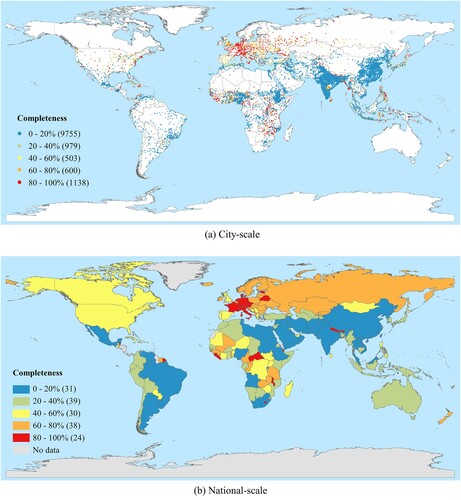
We can see from Figure 2a and 2b that more than 75% (9755/12975) of cities have an estimated OSM building completeness value between 0% and 20%. This indicates that there is a lack of OSM building data in most cities. In contrast, approximately 13% (1738/12975) of cities have an estimated OSM building completeness value higher than 60%; approximately 9% (1138/12975) of cities have an estimated value higher than 80%. The cities with relatively high completeness values of OSM building data are mostly located in Europe and Africa.

In terms of the national scale (Figure 2b and Appendix A), the OSM building completeness is lower than 20% for 31 out of the 162 countries. These countries are mostly located in North America (e.g. Brazil and Argentina), Africa (e.g. Egypt, Sudan, South Africa), and Asia (e.g. India and China). In contrast, for 62 out of the 162 countries, the OSM building completeness values are higher than 60%. They are mostly located in Europe (e.g. France and Germany), Africa (e.g. Central African Republic and Sierra Leone), and Russia.

Figure 3 shows the estimated OSM building completeness at grid scale for 15 cities worldwide (Appendix A). These cities are ranked according to their completeness values from the highest (95.2%) to the lowest (14.6%).

Figure 3. The estimated OSM building completeness of 15 typical cities worldwide.

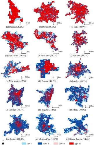
Figure 3 shows that the estimated (OSM building) completeness varies with different cities. Specifically, the estimated completeness values for six cities, i.e. Bangui (95.2%), Berlin (86.8%), Paris (84.9%), Nur-Sultan (79.1%), Auckland (74.1%), and Moscow (69.2%), are relatively high. This means that most of these cities have been mapped with OSM building data. Conversely, the estimated completeness values for another six cities, i.e. Santiago (38.3%), Bogota (37.6%), Sydney (20.1%), Beijing (17.4%), Mexico City (15.4%), and Rio de Janeiro (14.6%), are relatively low. This means that most of these cities have not been mapped with OSM building data. The cities with relatively high OSM building completeness values are mostly located in Africa (Bangui), Europe (Berlin and Pairs), and Russia (Moscow and Nur-Sultan). Those with a relatively low OSM building completeness are mostly located in South America (Santiago and Rio de Janeiro) and Asia (Beijing). The results are consistent with those found in Figure 2.

4.2. Results of evaluation

1. City-scale assessment

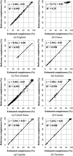
Figure 4 plots the linear relationships between the estimated and reference OSM building completeness values for the eight different countries. There is a high correlation (in most cases, the r-square varies from 0.986–0.998) between the estimated and the reference completeness values. Moreover, the slopes for the linear equations are almost all close to 1. This indicates that for each city, the estimated completeness is close to the reference completeness. However, the r-square is extremely low (0.286) for France. This is probably because the OSM building completeness is relatively high (e.g. > 90%) for most cities in this country. Thus, it may be more difficult to estimate the relatively small difference (e.g. < 10%) among such completeness values.

Figure 4. Relationships between estimated and reference OSM building completeness values for eight different countries.

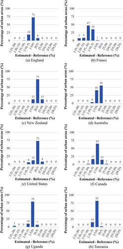
Figure 5 plots the distributions of the difference between estimated and reference OSM building completeness for each country. The difference is smaller than 5% for 80% – 90% of cities; it is smaller than 10% for 90% – 100% of cities. Although the difference is relatively large for France, the majority of the results verified that the estimated completeness is close to the reference completeness, which further verifies the effectiveness of the city-based assessment approach.

• (2) Grid-scale assessment

  Figure 5. Distributions of the difference between estimated and reference OSM building completeness for eight different countries.

  

Figure 6 shows the confusion matrixes of the eight countries, after comparing OSM and reference building completeness for the grid cells of all cities in a country. The overall accuracy (OA) varies from 78.1% (the lowest) to 90.9% (the highest). In six out of the eight countries, the OA is higher than 80%. The results verify the effectiveness of using population grid data as a proxy for reference building data. Moreover, in most cases, the user accuracy (UA) and producer accuracy (PA) are also close to or higher than 80%.

Figure 6. Confusion matrixes for eight different countries.

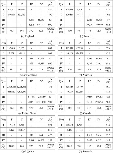
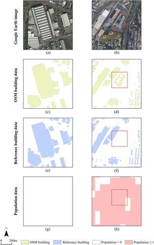
Nevertheless, the PA or UA may be much lower (e.g. 2.1% – 6.2%) for Type III. This is probably due to two reasons. In some regions (e.g. the industrial zone in Figure 7a), there are both OSM and reference building data (Figure 7c and 7e), but there is a lack of population count (Figure 7g), probably because the population grid data may indicate where people live, but few people live in the industrial zone. Thus, these regions were classified as Type III using the grid-based assessment, but they were classified as Type IV′ using the grid-based evaluation. For this case, the UA may be low. Conversely, in some regions (Figure 7b), there are both OSM building data and population count, but there is a lack of reference building data, probably due to the quality of the reference data. Thus, these regions were classified as Type IV using the grid-based assessment, but they were classified as Type III′ using the grid-based evaluation. For this case, the PA may be low.

Figure 7. Illustrating the reasons for the low accuracy of Type III, by comparing (a, b) Google Earth images, (c, d) OpenStreetMap (OSM) building data, (e, f) reference building data, and (g, h) population grid data.

Table 3 lists the confusion matrixes for 10,000 sampled grid cells. Although the user accuracy is still low for Type III, the overall accuracy is 81.6%, which illustrates that in general the estimated completeness is effective. Besides, the relationship between the number of sampled grid cells and overall accuracy was also plotted (Figure 8). This figure shows that the overall accuracy tends to be stable (around 81-82%), while the number of sampled grid cells is larger than 1,500, which illustrates the effectiveness of using 10,000 sampled grid cells for the analysis.

Figure 8. Relationship between the number of sampled grid cells and overall accuracy.

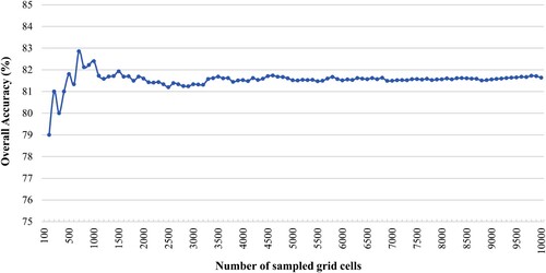
Table 3. Confusion matrixes for 10,000 sampled grid cells globally.

Type	I'	II'	III'	IV'	UA (%)
I	2,070	587	0	0	77.9
II	933	4,087	0	0	81.4
III	0	0	25	300	7.7
IV	0	0	16	1,982	99.2
PA (%)	68.9	87.4	61.0	86.9	OA (%) = 81.6

5. Discussion

5.1. Contributions

This study has three main contributions. First, a city-based assessment was proposed to quantitatively assess OSM building completeness for each city. Specifically, the ratio of grid cells that were mapped with OSM building data to those with estimated building data was calculated. This is an extension of the existing approach (Zhang et al. 2022), which had only investigated how to qualitatively determine whether a grid cell (e.g. 100-m resolution) has (or has not) been mapped with OSM building data. Nevertheless, other measures, e.g. the count ratio (number of OSM buildings divided by the number of reference buildings) and the area ratio (total OSM building area divided by the total reference building area), as reported by Törnros et al. (2015), also have been used to calculate OSM building completeness. For instance, Table 4 shows the linear relationship between the estimated completeness and the reference completeness that was calculated using the count ratio and the area ratio. This table indicates that the estimated completeness is much closer to the reference completeness when calculated using the area ratio; the corresponding r-square is above 0.9 in most cases. However, some individual buildings in the OSM dataset have been mapped as a combination in the reference dataset (Figure 9), which indicates that the number of buildings in OSM and reference datasets may be quite different. Thus, a relatively large difference between estimated and reference completeness has been observed using the count ratio (Table 4). From these results, we suggest using either the area ratio or our proposed measure (i.e. the ratio of grid cells) for assessing OSM building completeness.

Figure 9. Illustrating the flaw of using the count ratio for assessing OSM building completeness.

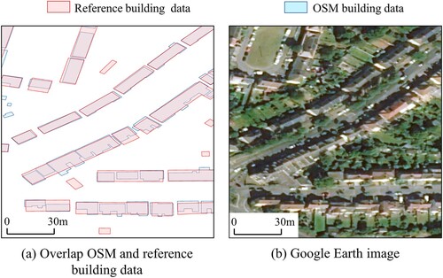
Table 4. Relationships between the estimated and reference OSM building completeness using the area ratio and count ratio.

Country	Area ratio	Count ratio
England	y = 0.98x + 0.00 (R^2= 0.950)	y = 2.13x − 0.43 (R^2= 0.781)
France	y = −0.05x + 1.02 (R^2= 0.009)	y = −0.24x + 1.20 (R^2= 0.020)
New Zealand	y = 0.92x − 0.03 (R^2= 0.997)	y = 1.55x − 0.47 (R^2= 0.980)
Australia	y = 1.04x − 0.01 (R^2= 0.995)	y = 1.23x − 0.13 (R^2= 0.979)
United States	y = 1.09x − 0.02 (R^2= 0.977)	y = 1.41x − 0.22 (R^2= 0.892)
Canada	y = 1.21x − 0.02 (R^2= 0.968)	y = 1.97x − 0.54 (R^2= 0.836)
Uganda	y = 1.32x − 0.00 (R^2= 0.938)	y = 1.78x − 0.13 (R^2= 0.838)
Tanzania	y = 1.03x + 0.01 (R^2= 0.998)	y = 1.70x − 0.10 (R^2= 0.870)

Second, the OSM building completeness has been documented for 12,975 cities worldwide. We found that the cities with a relatively high completeness are mostly located in Europe and Africa. This is because the OSM project originated in Europe, which has received significant attention and more edits by volunteers. Additionally, humanitarian mapping has been carried out in Africa through the OSM platform. Thus, there also is a relatively high data completeness in Africa. In contrast, the OSM building completeness is much lower (e.g. < 20%) for most other areas (Herfort et al. 2021). This is consistent with the results reported in several existing studies (Tian, Zhou, and Fu 2019; Zhou, Wang, and Liu 2022). All in all, although extensive studies have focused on assessing OSM building completeness, the global-scale completeness pattern has been uncovered in a quantitative way for the first time.

Third, a 100-m resolution dataset of OSM building completeness has been made available for the public use. This global dataset includes a total of 12,975 cities and may be not only beneficial for users to understand which cities and their grid cells have been mapped with OSM building data, but also for volunteers to discover where there still is a lack of building data in OSM and to provide/edit corresponding data.

5.2. Limitations

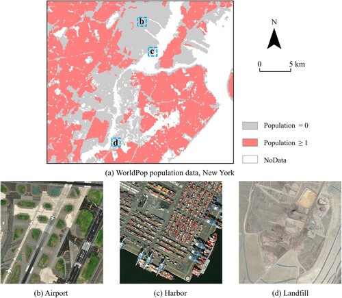
There are several limitations in this study. First, our approach uses population (grid) data for assessing OSM building completeness. Thus, the performance of our approach depends on the quality of the population data used. We have found that few people live in the industrial zones (Figure 7). Thus, there are flaws in using population data for OSM building completeness assessment. Although these flaws may be improved using a smaller threshold (e.g. zero) for the population count, other flaw(s) (e.g. there are population count but a lack of reference building data) may be increased (Figure 10). As suggested by Zhang et al. (2022), the threshold of one was used in our study. Alternatively, it may be possible to use other population data products (e.g. HRSL and Landscan⁵). However, the quality issue cannot be avoided; in fact, as discussed by Zhang et al. (2022), the 100-m resolution WorldPop data performed the best, especially in cities. Thus, the WorldPop dataset was used in our study. We also consulted the GHS-UCDB dataset because it can provide not only the extent of almost 13,000 cities across the globe, but also various attribute fields (e.g. city name and country name) for most cities. However, only 2015 urban centers were represented in the GHS-UCDB dataset. Despite this disadvantage, the temporal gap may impact less on the assessment results because the completeness values for most cities are lower than 20%. This means that even if the extent of a city becomes larger, the corresponding completeness may still be lower than 20%. Nevertheless, it is needed to expand the results with other latest datasets (Jiang et al. 2022).

Figure 10. Flaws of using a smaller threshold (zero) for the population count. “NoData” represents areas that were mapped as unsettled (Bondarenko et al. 2020).

Also, rural areas were not analyzed in our study because the population data may fail to detect population in rural areas, as reported in several existing studies (Leyk et al. 2019; Zhang et al. 2022). However, in future work, it would be worthwhile to propose effective approaches or to use high-quality datasets for assessing OSM building completeness in rural areas and also to investigate a global perspective.

Last but not least, we have provided an open dataset related to OSM building completeness in terms of 12,975 cities worldwide. However, this dataset was only validated using eight different countries and 10,000 sampled grid cells. The reference building data used for evaluation may also have flaws. Thus in future work not only more sampled grid cells but also more reliable reference building data will be needed for the validation. Conversely, the OSM data are being continually updated and, thus, the data may be outdated after it has been produced. Despite these disadvantages, it is possible to use the assessment approach and proposed measures to assess the completeness of OSM building data in an updated dataset.

6. Conclusion

This study assessed OSM building completeness of cities globally by employing population grid data as a proxy for reference building data (called the grid-based assessment), which was first proposed by Zhang et al. (2022). More importantly, the ratio of grid cells that mapped with OSM building data in proportion to those with estimated building data (called the city-based assessment) was proposed to assess OSM building completeness of each city. To be specific, 12,975 cities across the globe were analyzed, in terms of grid-based and city-based assessments. Then, the estimated OSM building completeness values were determined by comparing with reference building completeness, in terms of eight different countries worldwide and a large number (10,000) of sampled grid cells interpreted from Google Earth images. An open dataset related to OSM building completeness of the 12,975 cities was also produced for public use. The results showed that:

1. According to the spatial pattern of OSM building completeness, 75% of cities have a low completeness value (e.g. < 20%). In contrast, no more than 9% of cities have an estimated completeness value higher than 80%. The cities with a relatively high completeness value are mostly located in Europe (e.g. France and Germany) and Africa (e.g. Central African Republic and Sierra Leone).

2. From the performances of the assessment approaches, the overall accuracies of most studied countries were higher than 80% in terms of the grid-based assessment. The estimated completeness was highly correlated (e.g. r-square is larger than 0.99) to the reference completeness, in terms of the city-based assessment. Moreover, in most cases, the difference between estimated and reference completeness was smaller than 5%. The results verified the effectiveness of the grid-based and city-based assessments.

Further work will have two aims: first, other effective approaches may be proposed or other high-quality data products may be employed to assess OSM building completeness, especially in rural areas. Second, it is necessary to assess the quality of OSM building data in terms of not only completeness but also other measures (e.g. positional accuracy, attribute accuracy, and logical consistency).

Acknowledgements

We would like to express special thanks to the editor and all the anonymous reviewers for their valuable comments that have helped improve this paper substantially.

Disclosure statement

No potential conflict of interest was reported by the author(s).

Data availability

The data that support the findings of this study are openly available in figshare at https://figshare.com/s/8d4d92388cff90ed7f9f.

Additional information

Funding

The project was supported by National Natural Science Foundation of China (Grant No. 41771428), and the Director Fund of the International Research Center of Big Data for Sustainable Development Goals (Grant No. CBAS2022DF010).

Notes

1 https://www.ordnancesurvey.co.uk/business-government/products/open-map-local

2 https://nz-buildings.readthedocs.io/en/latest/introduction.html

3 https://geoservices.ign.fr/documentation/donnees/vecteur/bdtopo

4 https://ciesin.columbia.edu/data/hrsl

5 https://landscan.ornl.gov

Appendix A. A global view of selected typical (a) countries and (b) cities.

References

- Bagheri, H., M. Schmitt, and X. Zhu. 2019. “Fusion of Multi-Sensor-Derived Heights and OSM-Derived Building Footprints for Urban 3D Reconstruction.” ISPRS International Journal of Geo-Information 8 (4): 193.
- Barron, C., P. Neis, and A. Zipf. 2014. “A Comprehensive Framework for Intrinsic OpenStreetMap Quality Analysis.” Transactions in GIS 18 (6): 877–895.
- Bondarenko, M., D. Kerr, A. Sorichetta, and A. J. Tatem. 2020. “Data from: Census/projection-disaggregated gridded population datasets for 189 countries in 2020 using Built-Settlement Growth Model (BSGM) outputs” (dataset). WorldPop, University of Southampton, UK. Accessed December 11, 2022. https://hub.worldpop.org/doi/10.5258SOTON/WP00684.
- Boo, G., E. Darin, D. R. Leasure, C. A. Dooley, H. R. Chamberlain, A. N. Lázár, K. Tschirhart. 2022. “High-resolution Population Estimation Using Household Survey Data and Building Footprints.” Nature Communications 13 (1): 1–10. https://doi.org/10.1038/s41467-022-29094-x.
- Brovelli, M. A., and G. Zamboni. 2018. “A new Method for the Assessment of Spatial Accuracy and Completeness of OpenStreetMap Building Footprints.” ISPRS International Journal of Geo-Information 7 (8): 289.
- Dorn, H., T. Törnros, and A. Zipf. 2015. “Quality Evaluation of VGI Using Authoritative Data—A Comparison with Land use Data in Southern Germany.” ISPRS International Journal of Geo-Information 4 (3): 1657–1671.
- Fan, H., A. Zipf, Q. Fu, and P. Neis. 2014. “Quality Assessment for Building Footprints Data on OpenStreetMap.” International Journal of Geographical Information Science 28 (4): 700–719.
- Florczyk, A., C. Corbane, M. Schiavina, M. Pesaresi, L. Maffenini, M. Melchiorri, et al. 2019. “Data from: GHS Urban Centre Database 2015, multitemporal and multidimensional attributes, R2019A” (dataset). European Commission, Joint Research Centre (JRC) Accessed December 11, 2022. https://data.jrc.ec.europa.eu/dataset/53473144-b88c-44bc-b4a3-4583ed1f547e.
- Girres, J. F., and G. Touya. 2010. “Quality Assessment of the French OpenStreetMap Dataset.” Transactions in GIS 14 (4): 435–459.
- Goodchild, M. F. 2007. “Citizens as Sensors: The World of Volunteered Geography.” GeoJournal 69 (4): 211–221.
- Guo, H., Q. Shi, A. Marinoni, B. Du, and L. Zhang. 2021. “Deep Building Footprint Update Network: A Semi-Supervised Method for Updating Existing Building Footprint from bi-temporal Remote Sensing Images.” Remote Sensing of Environment 264: 112589.
- Haklay, M. 2010. “How Good is Volunteered Geographical Information? A Comparative Study of OpenStreetMap and Ordnance Survey Datasets.” Environment and Planning B: Planning and Design 37 (4): 682–703.
- Helbich, M., C. Amelunxen, P. Neis, and A. Zipf. 2012. “Comparative Spatial Analysis of Positional Accuracy of OpenStreetMap and Proprietary Geodata.” Proceedings of GI_Forum 4: 24.
- Herfort, B., S. Lautenbach, J. Porto de Albuquerque, J. Anderson, and A. Zipf. 2021. “The Evolution of Humanitarian Mapping Within the OpenStreetMap Community.” Scientific Reports 11 (1): 1–15.
- Heris, M. P., N. L. Foks, K. J. Bagstad, A. Troy, and Z. H. Ancona. 2020. “A Rasterized Building Footprint Dataset for the United States.” Scientific Data 7: 207.
- Hong, T., Y. Chen, X. Luo, N. Luo, and S. H. Lee. 2020. “Ten Questions on Urban Building Energy Modeling.” Building and Environment 168: 106508.
- Huang, X., C. Wang, Z. Li, and H. Ning. 2021. “A 100 m Population Grid in the CONUS by Disaggregating Census Data with Open-Source Microsoft Building Footprints.” Big Earth Data 5 (1): 112–133.
- Jiang, H., Z. Sun, H. Guo, Q. Xing, W. Du, and G. Cai. 2022. “A Standardized Dataset of Built-up Areas of China’s Cities with Populations Over 300,000 for the Period 1990–2015.” Big Earth Data 6 (1): 103–126. doi:10.1080/20964471.2021.1950351.
- Leyk, S., A. E. Gaughan, S. Adamo, A. Sherbinin, D. Balk, S. Freire, et al. 2019. “The Spatial Allocation of Population: A Review of Large-Scale Gridded Population Data Products and Their Fitness for Use.” Earth System Science Data 11 (3): 1385–1409.
- Li, W., C. He, J. Fang, J. Zheng, H. Fu, and L. Yu. 2019. “Semantic Segmentation-Based Building Footprint Extraction Using Very High-Resolution Satellite Images and Multi-Source GIS Data.” Remote Sensing 11 (4): 403.
- Li, X., T. Hu, P. Gong, S. Du, B. Chen, X. Li, and Q. Dai. 2021. “Mapping Essential Urban Land Use Categories in Beijing with a Fast Area of Interest (AOI)-Based Method.” Remote Sensing 13 (3): 477.
- Mooney, P., and P. Corcoran. 2014. “Has OpenStreetMap a Role in Digital Earth Applications?” International Journal of Digital Earth 7 (7): 534–553.
- Park, Y., and J. M. Guldmann. 2019. “Creating 3D City Models with Building Footprints and LIDAR Point Cloud Classification: A Machine Learning Approach.” Computers, Environment and Urban Systems 75: 76–89.
- Qiu, Y., X. Zhao, D. Fan, S. Li, and Y. Zhao. 2022. “Disaggregating Population Data for Assessing Progress of SDGs: Methods and Applications.” International Journal of Digital Earth 15 (1): 2–29.
- Reed, F. J., A. E. Gaughan, F. R. Stevens, G. Yetman, A. Sorichetta, and A. J. Tatem. 2018. “Gridded Population Maps Informed by Different Built Settlement Products.” Data 3 (3): 33.
- Reinhart, C. F., and C. C. Davila. 2016. “Urban Building Energy Modeling–A Review of a Nascent Field.” Building and Environment 97: 196–202.
- Senaratne, H., A. Mobasheri, A. L. Ali, C. Capineri, and M. Haklay. 2017. “A Review of Volunteered Geographic Information Quality Assessment Methods.” International Journal of Geographical Information Science 31 (1): 139–167.
- Shao, Z., P. Tang, Z. Wang, N. Saleem, S. Yam, and C. Sommai. 2020. “BRRNet: A Fully Convolutional Neural Network for Automatic Building Extraction from High-Resolution Remote Sensing Images.” Remote Sensing 12 (6): 1050.
- Stevens, F. R., A. E. Gaughan, C. Linard, and A. J. Tatem. 2015. “Disaggregating Census Data for Population Mapping Using Random Forests with Remotely-Sensed and Ancillary Data.” PLoS One 10 (2): e0107042.
- Tian, Y., Q. Zhou, and X. Fu. 2019. “An Analysis of the Evolution, Completeness and Spatial Patterns of OpenStreetMap Building Data in China.” ISPRS International Journal of Geo-Information 8 (1): 35.
- Törnros, T., H. Dorn, S. Hahmann, and A. Zipf. 2015. “Uncertainties of Completeness Measures in OpenStreetMap–A Case Study for Buildings in a Medium-Sized German City.” ISPRS Annals of the Photogrammetry, Remote Sensing and Spatial Information Sciences 2: 353.
- Wang, C., M. Ferrando, F. Causone, X. Jin, X. Zhou, and X. Shi. 2022. “Data Acquisition for Urban Building Energy Modeling: A Review.” Building and Environment 217: 109056.
- Wang, C., S. Wei, S. Du, D. Zhuang, Y. Li, X. Shi, et al. 2021. “A Systematic Method to Develop Three Dimensional Geometry Models of Buildings for Urban Building Energy Modeling.” Sustainable Cities and Society 71: 102998.
- Wang, S., Q. Zhou, and Y. Tian. 2020. “Understanding Completeness and Diversity Patterns of OSM-Based Land-use and Land-Cover Dataset in China.” ISPRS International Journal of Geo-Information 9 (9): 531.
- Xu, Y., L. Wu, Z. Xie, and Z. Chen. 2018. “Building Extraction in Very High Resolution Remote Sensing Imagery Using Deep Learning and Guided Filters.” Remote Sensing 10 (1): 144.
- Zhang, Y., Q. Zhou, M. A. Brovelli, and W. Li. 2022. “Assessing OSM Building Completeness Using Population Data.” International Journal of Geographical Information Science 36 (7): 1443–1466.
- Zhou, Q. 2018. “Exploring the Relationship Between Density and Completeness of Urban Building Data in OpenStreetMap for Quality Estimation.” International Journal of Geographical Information Science 32 (2): 257–281.
- Zhou, Q., and X. Jing. 2022. “Evaluation and Comparison of Open and High-Resolution LULC Datasets for Urban Blue Space Mapping.” Remote Sensing 14: 5764.
- Zhou, Q., S. Wang, and Y. Liu. 2022. “Exploring the Accuracy and Completeness Patterns of Global Land-Cover/Land-use Data in OpenStreetMap.” Applied Geography 145: 102742.