Mapping common and glossy buckthorns (Frangula alnus and Rhamnus cathartica) using multi-date satellite imagery WorldView-3, GeoEye-1 and SPOT-7

ABSTRACT

Buckthorns (Glossy buckthorn, Frangula alnus and common buckthorn, Rhamnus cathartica) represent a threat to biodiversity. Their high competitivity lead to the replacement of native species and the inhibition of forest regeneration. Early detection strategies are therefore necessary to limit invasive alien plant species’ impacts, and remote sensing is one of the techniques for early invasion detection. Few studies have used phenological remote sensing approaches to map buckthorn distribution from medium spatial resolution images. Those studies highlighted the difficulty of detecting buckthorns in low densities and in understory using this category of images. The main objective of this study was to develop an approach using multi-date very high spatial resolution satellite imagery to map buckthorns in low densities and in the understory in the Québec city area. Three machine learning classifiers (Support Vector Machines, Random Forest and Extreme Gradient Boosting) were applied to WorldView-3, GeoEye-1 and SPOT-7 satellite imagery. The Random Forest classifier performed well (Kappa = 0.72). The SVM and XGBoost's coefficient Kappa were 0.69 and 0.66, respectively. However, buckthorn distribution in understory was identified as the main limit to this approach, and LiDAR data could be used to improve buckthorn mapping in similar environments.

KEYWORDS:

• Invasive alien plant species
• remote sensing
• buckthorns
• multi-date satellite imagery
• machine learning

1. Introduction

Human activities and climatic variability are the main drivers for the introduction and spread of invasive alien plant species (IAPS) (Kumar Rai and Singh 2020; Langmaier and Lapin 2020; Paz-Kagan et al. 2019; Guido and Pillar 2017; Early et al. 2016). Their introduction, intentional or accidental, as well as their spread after installation, can lead to negative ecological, health and economic impacts. These impacts can include the replacement of native species, the costs of eradication interventions, devaluation of invaded properties and spontaneous or long-term health issues such as photodermatitis from contact with the sap of some IAPS such as giant hogweed (Heracleum mantegazzianum) (Lavoie, Guay, and Joerin 2014; Vilà et al. 2010; Mack et al. 2000).

Glossy buckthorn (Frangula alnus) and common buckthorn (Rhamnus cathartica) are native to Europe and were introduced in North America in the early nineteenth century. Initially used as windbreaks (Boettcher, Gautam, and Cook 2021; Becker, Zmijewski, and Crail 2013; Heneghan et al. 2006), both species are now considered invasive (Lavoie, Guay, and Joerin 2014). These IAPS colonize forest edges, understory, riverbanks and open environments (e.g. wastelands), the last of which promote very dense colonies (Lavoie, Guay, and Joerin 2014; Heneghan et al. 2006; Frapier, Eckert, and Lee 2004). These IAPS are also characterized by a particular phenology as their leaves appear very early in the spring and remain green late into the fall (Labonté et al. 2020; Becker, Zmijewski, and Crail 2013; Knight et al. 2007; Archibold, Brooks, and Delanoy 1997). Heneghan et al. (2006) also found that buckthorns alter the chemical properties of the soil as a result of altered moisture and accelerated organic matter transformation processes (e.g. nitrogen and carbon mineralization). These changes in organic matter cycling can subsequently cause an increase in pH and decrease of soil nutrient availability for other organisms (Knight et al. 2007). The main impacts of these IAPS in invaded areas are the loss of biodiversity, the facilitation of the establishment of new invasive species and the inhibition of forest regeneration (Lavoie, Guay, and Joerin 2014; Knight et al. 2007; Frapier, Eckert, and Lee 2004).

Buckthorns are more competitive and replace native species by reducing their regeneration. As an example, Frapier, Eckert, and Lee (2004) showed that sites with high buckthorn percentage cover (>90% cover), had fewer new pines (0.11 seedlings/m²) than sites without buckthorns (0.40 seedlings/m²) in a coniferous forest (Pinus sp.) of New Hampshire (USA). Replacement of native species is also facilitated by the high germination rate of buckthorns, which can reach 85% (Archibold, Brooks, and Delanoy 1997). Moreover, their photosynthesis rate can be up to twice that of native species’ which allows them to grow very rapidly in comparison (Kalkman, Simonton, and Dornbos 2019; Harrington, Brown, and Reich 1989). This high competitiveness (Boettcher, Gautam, and Cook 2021; Kalkman, Simonton, and Dornbos 2019) necessitates early detection strategies so that eradication interventions can be promptly performed. Positive identifications can be made by in situ inventories which are time consuming and expensive, especially when conducted in areas with limited access (Lawrence, Wood, and Sheley 2006). Remote sensing has the potential to reduce these constraints and improve detection of IAPS over large areas.

Only two studies that used remote sensing to map buckthorn distribution were found in the available literature. Labonté et al. (2020) used a phenological approach based on a series of six multi-date (April, June, August, September, October and November) Landsat-8 OLI images to map understory buckthorns in Richmond and Cookshire (Quebec, Canada) forests dominated by broadleaf deciduous and coniferous trees. An overall accuracy of 69% was obtained and this low performance was attributed to low levels of buckthorn cover and spectral mixing (Labonté et al. 2020). Becker, Zmijewski, and Crail (2013) used the same approach using a series of 49 Landsat 7 ETM+ and Landsat 5 TM images (January to December between 2001 and 2011) in Ohio and Michigan (USA) and obtained an overall accuracy of 88%. This high accuracy can be attributed to the study environment (oak openings) and high buckthorn density. Labonté et al. (2020) showed that the classification error decreased with the increase of buckthorn cover levels in the studied plots (plot size = 30 × 30 m), as the spectral mixing in the pixel is reduced. For example, this error was 20% when buckthorn cover was 75% or higher, but rose to 31% from 25% or higher coverage. These studies highlight the limits of detecting low density and understory buckthorns (i.e. low percentage cover in a pixel) using medium spatial resolution satellite imagery. Although the use of multi-date very high (VHR) and high spatial resolution (HR) images could improve classification accuracy (Labonté et al. 2020; Becker, Zmijewski, and Crail 2013), there are no studies to date that have incorporated these data to map low-density and understory buckthorns.

The main objective of this study is to explore and compare the use of multi-date HR and VHR satellite imagery in combination with machine learning classifiers to detect understory buckthorns at low density.

2. Material and methods

2.1. Study area

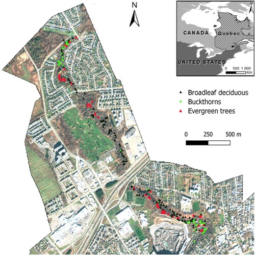
The study area is a 4 km long riparian zone located along the Beauport River in Quebec City (46°52′02″N, 71°12′35″W) (Figure 1). The canopy of the area is dominated by broadleaf deciduous trees: boxelder maple (Acer negundo), red maple (Acer rubrum), American elm (Ulmus americana), black willow (Salix nigra) and white birch (Betula papyrifera). A few patches of evergreen trees are present, mainly coniferous, including blue spruce (Picea pungens) and balsam fir (Abies balsamea). In this area, buckthorn presence is isolated, does not form homogeneous patches and are featured predominantly in the understory. We therefore chose this riparian zone as our study area for (1) the presence of many buckthorn individuals and (2) their spatial distribution (i.e. low density and understory) allowing us to test the detection efficiency of the VHR and HR images.

Figure 1. Study area and collected sample locations. The background is a true colour composite (red, green, blue) of a GeoEye-1 satellite image acquired on 5 November 2020.

2.2. Reference data

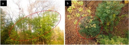
The collection of reference data was conducted during two periods: in the summer (26 June to 26 August 2020) and in late autumn (15–21 October 2021), when buckthorns are easily identifiable after most broadleaf deciduous trees have lost their leaves (Figure 2). Three classes of reference data were collected: buckthorn, evergreen, and broadleaf deciduous species. Two high-precision (≈1 m) Pro 6 H (Trimble, California) and Arrow Gold (EOS positioning system, Quebec) GNSS (Global Navigation Satellite Systems) receivers were used to locate and record the crown centre position of individuals of the three classes.

Figure 2. (a) Field (20 October 2021) and (b) drone (15 October 2021) photos of Buckthorns (red circle) understory. Source: Centre d’enseignement et de recherche en foresterie.

The broadleaf deciduous class corresponds to the dominant individual trees in the study area and samples were randomly located. Buckthorn and evergreen species were less numerous, and all accessible individuals were located. Buckthorns that were less than 4 metres tall or characterized by small crown surface were not used, as they are completely in the understory and could not be detected by remote sensing. The total number of points collected for each class was 54, 50, and 108 for buckthorn, evergreen and deciduous species, respectively.

2.3. Images acquisition and pre-processing

Three images acquired by WV-3/WV110 (WorldView-3 /World View 110 camera, 7 July 2020), SPOT-7/NAOMI (Satellite Pour l’Observation de la Terre-7, New AstroSat Optical Modular Instrument, 26 October 2019), and GeoEye-1/GIS (GeoEye Imaging System, 5 November 2020) satellites were used. The spectral and spatial characteristics of these images are presented in Table 1.

Table 1. Imagery specifications.

Satellite	Band	Wavelength range (centre) (nm)	Spatial resolution (m)
WV-3	Coastal	400–450 (425)	1.24
	Blue	450–510 (480)
	Green	510–580 (545)
	Yellow	585–625 (605)
	Red	630–690 (660)
	Red Edge	705–745 (725)
	Near-infrared	770–895 (832.5)
	Near-infrared	860–1040 (950)
	Panchromatic	450–800 (625)	0.31
SPOT-7	Blue	450–520 (485)
	Green	530–590 (560)
	Red	625–695 (660)	6
	Near-infrared	760–890 (825)
	Panchromatic	450–745 (597.5)	1.5
GeoEye-1	Blue	450–510 (480)
	Green	510–580 (545)
	Red	655–690 (672.5)	2
	Near-infrared	780–920 (850)
	Panchromatic	450–800 (625)	0.5

WV-3: WorldView3, SPOT-7: Satellite Pour l’Observation de la Terre -7.

Atmospheric corrections were performed using the ATCOR module (PCI Geomatics 2018) and fusion of the panchromatic band with the multispectral bands was performed using the ratio component substitution (RCS) fusion method available in the Orfeo toolbox (Deur, Gašparović, and Balenović 2021; Mhangara, Mapurisa, and Mudau 2020; Grizonnet et al. 2017).

A digital terrain model (Varin, Allostry, and Chalghaf 2020) at one-meter spatial resolution was used for orthorectification of the pansharpened images, and an orthomosaic of the WV-3 image was generated using the Bundle colour balancing method (PCI Geomatics 2018) from fourteen tiles.

Three masks were applied to remove unvegetated areas, shadows and vegetation less than 4 m tall. A first mask was created using the WV-3 image to remove water, bare soil and buildings by applying a normalized difference vegetation index (NDVI) threshold (NDVI < 0.37) based on the NDVI distribution of the field reference data. To remove shadows, a second mask was applied using a shadow index (SI) threshold (Zhou et al. 2018) (SI ≤ 13.13) based on SI analysis of shadow objects. A third mask was applied to remove vegetation below 4 metres in height using a digital height model at one-meter spatial resolution (Varin, Allostry, and Chalghaf 2020).

2.4. Segmentation

The GeoEye-1 image was used for segmentation because of its acquisition period (i.e. fall) that maximizes the distinction between buckthorns and other species (i.e. buckthorns leaves remain green late in the fall) and its better spatial resolution than the SPOT-7 image taken during the same season. The multi-resolution algorithm was selected for segmentation due to its performance in several recent image segmentation studies (Lourenço et al. 2021; Chen, Chen, and Jing 2021; Jombo, Adam, and Odindi 2021).

The segmentation parameter values (i.e. scale, colour, and compactness) were determined using an iterative trial-and-error process combined with the estimation of scale parameter (ESP2) method (Drăguţ et al. 2014; Fernandes et al. 2014; Müllerová, Pergl, and Pyšek 2013; Jones et al. 2011; Drǎguţ, Tiede, and Levick 2010). Scale, colour, and compactness were set to 5, 0.9 and 0.5, respectively. Blue and green bands weights were each set to 1 while red and near-infrared bands were set to 2.

Spectral, textural, and geometric arithmetic features were extracted from the objects resulting from the segmentation (Table 2). A total of 150 features for WV-3 and 77 for each of the SPOT-7 and GeoEye-1 images were calculated, for a total of 304. The features were centred and scaled and a correlation analysis was performed to eliminate correlated features using a Pearson coefficient greater than or equal to 0.85 (Varin, Chalghaf, and Joanisse 2020). The Jeffries Matusita (JM) separability distance was used to select the most relevant features among two correlated ones.

Table 2. Features used for classification.

Category	Feature	Band combination	References
Spectral	Mean	All
	Maximum	All
	Standard deviation	All
	95th percentile	All
	Skewness	All
	NDVI (Normalized Difference Vegetation Index)	(NIR – red) / (NIR + RE)	Carlson and Ripley (1997); Jombo, Adam, and Odindi (2021); Yan et al. (2018)
	RENDVI (Red-Edge Normalized Difference Vegetation Index)	(NIR – RE) / (NIR + RE)	Waser et al. (2014)
	VARI (Visible Atmospherically Resistant Index)	(green – red) / (green + red – blue)	Gitelson et al. (2002)
	RGR (Red Green Ratio)	red / green	Zhou et al. (2021)
	SR (Simple Ratio)	NIR /rouge	Zhou et al. (2021)
	BTBR (Bi-Temporal Band Ratio)	red, green*	Dorigo et al. (2012)
	HSI (Hue, Saturation, Intensity)	red, green, blue*	Chaudhary et al. (2012)
	CI (Colour Index)	(red – green) / (red + green)	Escadafal and Huete (1991)
	BI (Brightness index)	(red^2 + NIR^2)^0.5	Zhou et al. (2018)
Textural	GLCM (Gray Level Co-occurrence Matrix): contrast, correlation, entropy, homogeneity, angular second moment, mean, standard deviation GLDV (Gray Level Difference Vector): contrast, entropy, mean, angular second moment	All	Haralick (1979)
Geometric	Width, length, compactness	–	–

NIR: Near-infrared, RE: Red-Edge.

*Because of limited space, only used bands are presented (see references for detailed definition).

2.5. Classification approach and optimization of machine learning classifiers

Object-based classification was performed following a multi-date approach by combining the three images and the BTBR (Bi-Temporal Band Ratio) (WV-3 + SPOT-7 + GeoEye-1 + BTBR). Object-based classification consists of first grouping homogeneous neighbouring pixels into objects which will then be classified (Chen, Zhao, and Powers 2014). This approach has the advantage of using spectral, geometric, textural, and topologic features in the classification process (Hantson, Kooistra, and Slim 2012). It also avoids the salt-and-pepper noise frequently observed in images at very high spatial resolutions (Hirayama et al. 2019; Chen, Zhao, and Powers 2014; Jones et al. 2011). The BTBR (equation 1) developed by Dorigo et al. (2012) and used for multi-date classification was calculated between WV-3 and each of the other two images (BTBR1: WV-3 and GeoEye-1, BTBR2: WV-3 and SPOT-7), (1) $\mathrm{BTBR}={\displaystyle \frac{{\displaystyle \frac{R_{\mathrm{off}}}{R_{\mathrm{on}}}-{\displaystyle \frac{G_{\mathrm{off}}}{G_{\mathrm{on}}}}}}{{\displaystyle \frac{R_{\mathrm{off}}}{R_{\mathrm{on}}}+{\displaystyle \frac{G_{\mathrm{off}}}{G_{\mathrm{on}}}}}}}$(1) where R and G indicate reflectance values in the red and green bands, respectively. The suffixes indicate the image acquisition period (growing season (on) and senescence period (off)).

Random Forest (RF) (Breiman 2001), Support Vector Machines (SVM) (Guenther and Schonlau 2016) and Extreme Gradient Boosting (XGBoost) (Zarei, Hasanlou, and Mahdianpari 2021; Samat et al. 2020) classifiers were used for classification and compared. The selection of relevant discriminant features for each classifier was performed using the recursive feature elimination selection method (Yang et al. 2019; Guyon, Weston, and Barnhill 2002; Ambroise and McLachlan 2002) and is detailed in Nininahazwe, Varin, and Théau (2022). The caret library in R (R core team 2021) was used to optimize the number of random features used at each node (mtry) and the number of decision trees (ntree) for the RF classifier. The radial basis function showed good performances in previous studies (Jombo et al. 2020; Qian et al. 2015; Huang, Davis, and Townshend 2002) and was therefore used in this study for SVM kernel function. The SVM's cost and sigma parameters as well as the XGBoost parameters, such as the learning rate, were automatically optimized using the caret library (R core team 2021). The optimal values selected were presented in the Appendix 1.

2.6. Classification accuracy assessment

The segments were overlaid on the reference data, and 70% of each class was used to train the models while 30% of the segments were used for validation. Cohen's Kappa coefficient (Congalton 1991; Cohen 1960), overall accuracy, and the F1-score (i.e. the harmonic mean of user and producer accuracy) (Costa et al. 2021; Yang 2001) were used to evaluate the accuracy of the models. The output of the models is a membership probability between 0 and 1 for each class. The sum of the class probabilities is equal to 1. The membership of the object was the class with the highest probability.

3. Results and discussion

The multi-date classification performed in this study shows that the RF classifier performs better (Kappa = 0.72) compared to the other classifiers (Kappa = 0.69 (SVM); 0.66 (XGBoost)) (Table 3).

Table 3. Performance measures of classifiers. Values in bold indicate the maximum performance values.

	GeoEye-1 + WV-3 + SPOT-7 + BTBR1+ BTBR2*
		RF	SVM	XGBoost
Global	Kappa	0.72	0.69	0.66
	OA	0.83	0.82	0.80
Buckthorns	UA	0.67	0.67	0.67
	PA	0.57	0.43	0.43
	F1-score	0.62	0.52	0.52
Evergreen trees	UA	0.93	0.93	0.93
	PA	0.93	1.00	0.93
	F1-score	0.93	0.97	0.93
Broadleaf deciduous	UA	0.85	0.81	0.78
	PA	0.91	0.91	0.91
	F1-score	0.88	0.85	0.84
Mean F1-score		0.81	0.78	0.76
Standard deviation		0.13	0.17	0.16

BTBR: Bi-Temporal Band Ratio, *BTBR1: WV-3 and GeoEye-1, BTBR2: WV-3 and SPOT-7; RF: Random Forest, SVM: Support vector machines, XGBoost: Extreme gradient boosting; OA: Overall Accuracy, UA: User Accuracy, PA: Producer Accuracy.

For individual class performance, buckthorns are less well detected compared to the other classes regardless of the classifier used. In particular, the optimal classifier (RF) for buckthorns reaches 0.62 (F1-score) compared to 0.93 and 0.88 for broadleaf deciduous and evergreen species, respectively (Table 3). This low F1-score value results from omission errors (43%, 1-producer accuracy) and commission errors (33%, 1 – user accuracy). The omission errors indicate the difficulty of the classifier to predict some buckthorns, while the commission errors show that some absences (e.g. broadleaf deciduous or evergreen species) were erroneously classified as buckthorns. The spatial distribution of buckthorns in the study area probably accounts for these errors. Although individuals less than 4 m tall were eliminated from the analyses, buckthorns are always found below the canopy of other dominant and taller broadleaf deciduous trees, so branches and trunks of other overhanging trees would contribute strongly to the pixel reflectance (Labonté et al. 2020). Broadleaf deciduous trees (e.g. black willow) were also observed with green leaves late in the fall, which could contribute to misclassification.

Our results produced higher levels of accuracy (overall accuracy = 83%) compared to studies conducted in similar conditions (Labonté et al. 2020) (overall accuracy = 69%). The relatively low performance of the study conducted by Labonté et al. (2020) was related to the spectral mixing occurring in pixels at medium spatial resolution images they used (Landsat 8 OLI). In that case, buckthorn individuals’ size was smaller than that of the pixels (Labonté et al. 2020). The VHR used in our study therefore appear to have reduced the effects of spectral mixing.

On the other hand, our results (OA: 83%, Kappa: 0.72) are comparable to those found by Becker, Zmijewski, and Crail (2013) who detected buckthorns in a more favourable context (i.e. open environment and high densities) than ours (OA: 88%, Kappa: 0.73). Considering the detection challenges (i.e. mapping low-density and understory buckthorns) in our study area, our multi-date classification approach is performing well, although improvements are needed to produce a more accurate map that can be used directly by managers.

In addition, fifteen features used by the optimal classifier highlight the relevance of the multi-date classification approach. The features calculated from the WV-3 and GeoEye-1 images contributed in similar proportions (6/15 for WV-3 and 7/15 for GeoEye-1), in addition to the BTBR calculated between these two images (BTBR1). However, the contribution of the features calculated from SPOT-7 is less significant (1/15). This could be due to the low spatial resolution of the multispectral SPOT-7 bands (6 m, before pansharpening) compared to those from GeoEye-1 (2 m) and WV-3 (1.24 m), hence the advantage of using VHR images in the development of buckthorn mapping methods. Our study also highlights the low relevance of adding lower resolution images to VHR images acquired during the same period.

In environments similar to our study area, the omission and commission errors could be reduced using other data sources, such as high-density point clouds from LiDAR (Light Detection and Ranging) acquired in the fall season. This technology had not yet been applied for buckthorn detection, although they have been used successfully in previous vegetation mapping studies (Guo et al. 2022; Jombo, Adam, and Tesfamichael 2022; Budei et al. 2018; Dalponte, Bruzzone, and Gianelle 2008; Asner et al. 2008). In particular, high density or multiple-return LiDAR would allow for the derivation of several structural features (e.g. crown shape and area), identification of crowns at different heights (Shi et al. 2018), and the extraction of several radiometric features derived from backscattered signal intensity (Shi et al. 2018; Ørka, Næsset, and Bollandsås 2009; Dalponte et al. 2009; Dalponte, Bruzzone, and Gianelle 2008; Asner et al. 2008). These features could be incorporated into optical images to improve remote sensing mapping approaches for buckthorns in understory and at low density. Features such as height could allow for a more accurate removal of unsuitable vegetation strata using a canopy height model (Asner et al. 2008), while radiometric features could be used for discrimination between buckthorns and native species (Shi et al. 2018; Ørka, Næsset, and Bollandsås 2009; Dalponte, Bruzzone, and Gianelle 2008).

4. Conclusion

The mapping performances of low-density understory buckthorns using multi-date VHR and HR images are satisfactory in comparison with similar previous studies. However, the use of this multi-date approach in an operational context (e.g. target intervention areas) would require improvements to reduce the errors and thereby target the problematic areas more precisely. Future studies could incorporate LiDAR data as well as multispectral images at centimetre resolution (e.g. drone images) to improve buckthorn detection in understory.

Acknowledgments

The authors gratefully acknowledge Nicolas Turcotte-Major (Ville de Québec), Anne-Marie Dubois (CERFO), Camille Armellin (CERFO), Jean Marchal (CERFO), Maryam Rashidfar (CERFO), Julie Deslandes (Ville de Québec) and Ramdani Mustapha (Ville de Québec) for their support during the project.

Disclosure statement

No potential conflict of interest was reported by the author(s).

Data availability statement

The data that support the findings of this study are openly available in the Open Science Framework data repository.

Additional information

Funding

This work was supported by the Mitacs Accélération program, award number IT16759 and by the Ville de Québec.

Appendix 1.

Used hyperparameters for Extreme Gradient Boosting (XGBoost), Support Vector Machines (SVM) and Random Forest (RF)

Table

Classifier	Hyperparameter	Optimal value
XGBoost	Nrounds	100
	Max depth	8
	Learning rate	0.4
	Gamma	0
	Colsample_bytree	0.8
	min_child_weight	1
	Subsample	0.88
	Number of features selected	30
RF	Mtry	7
	Ntree	400
	Number of features selected	25
SVM	Sigma	0.04
	Cost	4
	Number of features selected	20

References

- Ambroise, C., and G. J. McLachlan. 2002. “Selection Bias in Gene Extraction on the Basis of Microarray Gene-Expression Data.” Proceedings of the National Academy of Sciences 99 (10): 6562–6566. doi:10.1073/pnas.102102699.
- Archibold, O. W., D. Brooks, and L. Delanoy. 1997. “An Investigation of the Invasive Shrub European Buckthorn, Rhamnus cathartica L., Near Saskatoon, Saskatchewan.” Canadian Field-Naturalist 111 (4): 617–621. https://www.researchgate.net/profile/Darin-Brooks/publication/239951389_An_investigation_of_the_invasive_shrub_European_Buckthorn_Rhamnus_cathartica_L_near_Saskatoon_Saskatchewan/links/54621dd30cf2c1a63c0295e2/An-investigation-of-the-invasive-shrub-European-Buckthorn-Rhamnus-cathartica-L-near-Saskatoon-Saskatchewan.pdf.
- Asner, G. P., D. E. Knapp, T. Kennedy-Bowdoin, M. O. Jones, R. E. Martin, J. Boardman, and R. F. Hughes. 2008. “Invasive Species Detection in Hawaiian Rainforests Using Airborne Imaging Spectroscopy and LiDAR.” Remote Sensing of Environment 112 (5): 1942–1955. doi:10.1016/j.rse.2007.11.016.
- Becker, R. H., K. A. Zmijewski, and T. Crail. 2013. “Seeing the Forest for the Invasives: Mapping Buckthorn in the Oak Openings.” Biological Invasions 15 (2): 315–326. doi:10.1007/s10530-012-0288-8.
- Boettcher, T. J., S. Gautam, and J. Cook. 2021. “The Impact of Invasive Buckthorn on Ecosystem Services and Its Potential for Bioenergy Production: A Review.” Journal of Sustainable Forestry, 1–23. doi:10.1080/10549811.2021.1992637.
- Breiman, L. 2001. “Random Forests.” Machine Learning 45 (1): 5–32. doi:10.1023/A:1010933404324.
- Budei, B. C., B. St-Onge, C. Hopkinson, and F. A. Audet. 2018. “Identifying the Genus or Species of Individual Trees Using a Three-Wavelength Airborne Lidar System.” Remote Sensing of Environment 204: 632–647. doi:10.1016/j.rse.2017.09.037.
- Carlson, T. N., and D. A. Ripley. 1997. “On the Relation Between NDVI, Fractional Vegetation Cover, and Leaf Area Index.” Remote Sensing of Environment 62 (3): 241–252. doi:10.1016/S0034-4257(97)00104-1.
- Chaudhary, P., A. K. Chaudhari, A. N. Cheeran, and S. Godara. 2012. “Color Transform Based Approach for Disease Spot Detection on Plant Leaf.” International Journal of Computer Science and Telecommunications 3 (6): 65–70. http://www.ijcst.org/Volume3/Issue6/p12_3_6.pdf.
- Chen, Y., Q. Chen, and C. Jing. 2021. “Multi-resolution Segmentation Parameters Optimization and Evaluation for VHR Remote Sensing Image Based on Mean NSQI and Discrepancy Measure.” Journal of Spatial Science 66 (2): 253–278. doi:10.1080/14498596.2019.1615011.
- Chen, G., K. Zhao, and R. Powers. 2014. “Assessment of the Image Misregistration Effects on Object-Based Change Detection.” ISPRS Journal of Photogrammetry and Remote Sensing 87: 19–27. doi:10.1016/j.isprsjprs.2013.10.007.
- Cohen, J. 1960. “A Coefficient of Agreement for Nominal Scales.” Educational and Psychological Measurement 20 (1): 37–46. doi:10.1177/001316446002000104.
- Congalton, R. G. 1991. “A Review of Assessing the Accuracy of Classifications of Remotely Sensed Data.” Remote Sensing of Environment 37 (1): 35–46. doi:10.1016/0034-4257(91)90048-B.
- Costa, M. V. C. V., O. L. F. Carvalho, A. G. Orlandi, I. Hirata, A. O. Albuquerque, F. V. Silva, R. F. Guimarães, R. A. T. Gomes, and O. A. C. Júnior. 2021. “Remote Sensing for Monitoring Photovoltaic Solar Plants in Brazil Using Deep Semantic Segmentation.” Energies 14 (10): 2960. doi:10.3390/en14102960.
- Dalponte, M., L. Bruzzone, and D. Gianelle. 2008. “Fusion of Hyperspectral and LIDAR Remote Sensing Data for Classification of Complex Forest Areas.” IEEE Transactions on Geoscience and Remote Sensing 46 (5): 1416–1427. doi:10.1109/TGRS.2008.916480.
- Dalponte, M., N. C. Coops, L. Bruzzone, and D. Gianelle. 2009. “Analysis on the Use of Multiple Returns LiDAR Data for the Estimation of Tree Stems Volume.” IEEE Journal of Selected Topics in Applied Earth Observations and Remote Sensing 2 (4): 310–318. doi:10.1109/JSTARS.2009.2037523.
- Deur, M., M. Gašparović, and I. Balenović. 2021. “An Evaluation of Pixel- and Object-Based Tree Species Classification in Mixed Deciduous Forests Using Pansharpened Very High Spatial Resolution Satellite Imagery.” Remote Sensing 13 (10): 1868. doi:10.3390/rs13101868.
- Dorigo, W., A. Lucieer, T. Podobnikar, and A. Čarni. 2012. “Mapping Invasive Fallopia Japonica by Combined Spectral, Spatial, and Temporal Analysis of Digital Orthophotos.” International Journal of Applied Earth Observation and Geoinformation 19: 185–195. doi:10.1016/j.jag.2012.05.004.
- Drăguţ, L., O. Csillik, C. Eisank, and D. Tiede. 2014. “Automated Parameterisation for Multi-Scale Image Segmentation on Multiple Layers.” ISPRS Journal of Photogrammetry and Remote Sensing 88: 119–127. doi:10.1016/j.isprsjprs.2013.11.018.
- Drǎguţ, L., D. Tiede, and S. R. Levick. 2010. “ESP: A Tool to Estimate Scale Parameter for Multiresolution Image Segmentation of Remotely Sensed Data.” International Journal of Geographical Information Science 24 (6): 859–871. doi:10.1080/13658810903174803.
- Early, R., B. A. Bradley, J. S. Dukes, J. J. Lawler, J. D. Olden, D. M. Blumenthal, P. Gonzalez, et al. 2016. “Global Threats from Invasive Alien Species in the Twenty-First Century and National Response Capacities.” Nature Communications 7 (1): 12485. doi:10.1038/ncomms12485.
- Escadafal, R., and A. Huete. 1991. “Etude des Propriétés Spectrales des Sols Arides Appliquée à l’Amélioration des Indices de Végétation Obtenus par Télédétection.” Comptes rendus de l’Académie des sciences. Série 2, Mécanique, Physique, Chimie, Sciences de l’univers, Sciences de la Terre 312 (11): 1385–1391. http://pascal-francis.inist.fr/vibad/index.php?action=getRecordDetail&idt=5058337.
- Fernandes, M. R., F. C. Aguiar, J. M. N. Silva, M. T. Ferreira, and J. M. C. Pereira. 2014. “Optimal Attributes for the Object Based Detection of Giant Reed in Riparian Habitats: A Comparative Study Between Airborne High Spatial Resolution and WorldView-2 Imagery.” International Journal of Applied Earth Observation and Geoinformation 32: 79–91. doi:10.1016/j.jag.2014.03.026.
- Frapier, B., R. T. Eckert, and T. D. Lee. 2004. “Experimental Removal of the Non-Indigenous Shrub Rhamnus Frangula (Glossy Buckthorn): Effects on Native Herbs and Woody Seedlings.” Northeastern Naturalist 11 (3): 333–342. doi:10.1656/1092-6194(2004)011[0333:EROTNS]2.0.CO;2.
- Gitelson, A. A., Y. J. Kaufman, R. Stark, and D. Rundquist. 2002. “Novel Algorithms for Remote Estimation of Vegetation Fraction.” Remote Sensing of Environment 80 (1): 76–87. doi:10.1016/S0034-4257(01)00289-9.
- Grizonnet, M., J. Michel, V. Poughon, J. Inglada, M. Savinaud, and R. Cresson. 2017. “Orfeo ToolBox: Open Source Processing of Remote Sensing Images.” Open Geospatial Data, Software and Standards 2 (1): 15. doi:10.1186/s40965-017-0031-6.
- Guenther, N., and M. Schonlau. 2016. “Support Vector Machines.” The Stata Journal: Promoting Communications on Statistics and Stata 16 (4): 917–937. doi:10.1177/1536867X1601600407.
- Guido, A., and V. D. Pillar. 2017. “Invasive Plant Removal: Assessing Community Impact and Recovery from Invasion.” Journal of Applied Ecology 54 (4): 1230–1237. doi:10.1111/1365-2664.12848.
- Guo, Y., H. Zhang, Q. Li, Y. Lin, and J. Michalski. 2022. “New Morphological Features for Urban Tree Species Identification Using LiDAR Point Clouds.” Urban Forestry & Urban Greening 71: 127558. doi:10.1016/j.ufug.2022.127558.
- Guyon, I., J. Weston, and S. Barnhill. 2002. “Gene Selection for Cancer Classification Using Support Vector Machines.” Machine Learning 46: 389–422. doi:10.1023/A:1012487302797.
- Hantson, W., L. Kooistra, and P. A. Slim. 2012. “Mapping Invasive Woody Species in Coastal Dunes in the Netherlands: A Remote Sensing Approach Using LIDAR and High-Resolution Aerial Photographs.” Applied Vegetation Science 15 (4): 536–547. doi:10.1111/j.1654-109X.2012.01194.x.
- Haralick, R. M. 1979. “Statistical and Structural Approaches to Texture.” Proceedings of the IEEE 67 (5): 786–804. doi:10.1109/PROC.1979.11328.
- Harrington, R. A., B. J. Brown, and P. B. Reich. 1989. “Ecophysiology of Exotic and Native Shrubs in Southern Wisconsin: I. Relationship of Leaf Characteristics, Resource Availability, and Phenology to Seasonal Patterns of Carbon Gain.” Oecologia 80 (3): 356–367. doi:10.1007/BF00379037.
- Heneghan, L., F. Fatemi, L. Umek, K. Grady, K. Fagen, and M. Workman. 2006. “The Invasive Shrub European Buckthorn (Rhamnus cathartica, L.) Alters Soil Properties in Midwestern U.S. Woodlands.” Applied Soil Ecology 32 (1): 142–148. doi:10.1016/j.apsoil.2005.03.009.
- Hirayama, H., R. C. Sharma, M. Tomita, and K. Hara. 2019. “Evaluating Multiple Classifier System for the Reduction of Salt-and-Pepper Noise in the Classification of Very-High-Resolution Satellite Images.” International Journal of Remote Sensing 40 (7): 2542–2557. doi:10.1080/01431161.2018.1528400.
- Huang, C., L. S. Davis, and J. R. G. Townshend. 2002. “An Assessment of Support Vector Machines for Land Cover Classification.” International Journal of Remote Sensing 23 (4): 725–749. doi:10.1080/01431160110040323.
- Jombo, S., E. Adam, M. J. Byrne, and S. W. Newete. 2020. “Evaluating the Capability of Worldview-2 Imagery for Mapping Alien Tree Species in a Heterogeneous Urban Environment.” Cogent Social Sciences 6 (1): 1754146. doi:10.1080/23311886.2020.1754146.
- Jombo, S., E. Adam, and J. Odindi. 2021. “Classification of Tree Species in a Heterogeneous Urban Environment Using Object-Based Ensemble Analysis and World View-2 Satellite Imagery.” Applied Geomatics 13 (3): 373–387. doi:10.1007/s12518-021-00358-3.
- Jombo, S., E. Adam, and S. Tesfamichael. 2022. “Classification of Urban Tree Species Using LiDAR Data and WorldView-2 Satellite Imagery in a Heterogeneous Environment.” Geocarto International, 1–24. doi:10.1080/10106049.2022.2028904.
- Jones, D., S. Pike, M. Thomas, and D. Murphy. 2011. “Object-Based Image Analysis for Detection of Japanese Knotweed s.l. Taxa (Polygonaceae) in Wales (UK).” Remote Sensing 3 (2): 319–342. doi:10.3390/rs3020319.
- Kalkman, J. R., P. Simonton, and D. L. Dornbos. 2019. “Physiological Competitiveness of Common and Glossy Buckthorn Compared with Native Woody Shrubs in Forest Edge and Understory Habitats.” Forest Ecology and Management 445: 60–69. doi:10.1016/j.foreco.2019.05.007.
- Knight, K. S., J. S. Kurylo, A. G. Endress, J. R. Stewart, and P. B. Reich. 2007. “Ecology and Ecosystem Impacts of Common Buckthorn (Rhamnus cathartica): A Review.” Biological Invasions 9 (8): 925–937. doi:10.1007/s10530-007-9091-3.
- Kumar Rai, P., and J. S. Singh. 2020. “Invasive Alien Plant Species: Their Impact on Environment, Ecosystem Services and Human Health.” Ecological Indicators 111: 106020. doi:10.1016/j.ecolind.2019.106020
- Labonté, J., G. Drolet, J.-D. Sylvain, N. Thiffault, F. Hébert, and F. Girard. 2020. “Phenology-Based Mapping of an Alien Invasive Species Using Time Series of Multispectral Satellite Data: A Case-Study with Glossy Buckthorn in Québec, Canada.” Remote Sensing 12 (6): 922. doi:10.3390/rs12060922.
- Langmaier, M., and K. Lapin. 2020. “A Systematic Review of the Impact of Invasive Alien Plants on Forest Regeneration in European Temperate Forests.” Frontiers in Plant Science 11: 524969. doi:10.3389/fpls.2020.524969.
- Lavoie, C., G. Guay, and F. Joerin. 2014. “Une Liste des Plantes Vasculaires Exotiques Nuisibles du Québec: Nouvelle Approche pour la Sélection des Espèces et l’Aide à la Décision.” Écoscience 21 (2): 133–156. doi:10.2980/21-2-3703.
- Lawrence, R. L., S. D. Wood, and R. L. Sheley. 2006. “Mapping Invasive Plants Using Hyperspectral Imagery and Breiman Cutler Classifications (RandomForest).” Remote Sensing of Environment 100 (3): 356–362. doi:10.1016/j.rse.2005.10.014
- Lourenço, P., A. C. Teodoro, J. A. Gonçalves, J. P. Honrado, M. Cunha, and N. Sillero. 2021. “Assessing the Performance of Different OBIA Software Approaches for Mapping Invasive Alien Plants Along Roads with Remote Sensing Data.” International Journal of Applied Earth Observation and Geoinformation 95: 102263. doi:10.1016/j.jag.2020.102263.
- Mack, R. N., D. Simberloff, W. Mark Lonsdale, H. Evans, M. Clout, and F. A. Bazzaz. 2000. “Biotic Invasions: Causes, Epidemiology, Global Consequences, and Control.” Ecological Applications 10 (3): 689–710. doi:10.1890/1051-0761(2000)010[0689:bicegc]2.0.co;2.
- Mhangara, P., W. Mapurisa, and N. Mudau. 2020. “Comparison of Image Fusion Techniques Using Satellite Pour l’Observation de la Terre (SPOT) 6 Satellite Imagery.” Applied Sciences 10 (5): 1881. doi:10.3390/app10051881.
- Müllerová, J., J. Pergl, and P. Pyšek. 2013. “Remote Sensing as a Tool for Monitoring Plant Invasions: Testing the Effects of Data Resolution and Image Classification Approach on the Detection of a Model Plant Species Heracleum Mantegazzianum (Giant Hogweed).” International Journal of Applied Earth Observation and Geoinformation 25: 55–65. doi:10.1016/j.jag.2013.03.004.
- Nininahazwe, F., M. Varin, and J. Théau. 2022. “Mapping Invasive Alien Plant Species with Very High Spatial Resolution and Multi-Date Satellite Imagery Using Object-Based and Machine Learning Techniques: A Comparative Study.” (in revision).
- Ørka, H. O., E. Næsset, and O. M. Bollandsås. 2009. “Classifying Species of Individual Trees by Intensity and Structure Features Derived from Airborne Laser Scanner Data.” Remote Sensing of Environment 113 (6): 1163–1174. doi:10.1016/j.rse.2009.02.002.
- Paz-Kagan, T., M. Silver, N. Panov, and A. Karnieli. 2019. “Multispectral Approach for Identifying Invasive Plant Species Based on Flowering Phenology Characteristics.” Remote Sensing 11 (8): 953. doi:10.3390/rs11080953.
- Qian, Y., W. Zhou, J. Yan, W. Li, and L. Han. 2015. “Comparing Machine Learning Classifiers for Object-based Land Cover classification Using very High Resolution Imagery.” Remote Sensing 7 (1): 153–168. doi: 10.3390/rs70100153.
- R Core Team. 2021. A Language and Environment for Statistical Computing. R Foundation for Statistical Computing, Vienna, Austria. https://www.R-project.org/.
- Samat, A., E. Li, W. Wang, S. Liu, C. Lin, and J. Abuduwaili. 2020. “Meta-XGBoost for Hyperspectral Image Classification Using Extended MSER-Guided Morphological Profiles.” Remote Sensing 12 (12): 1973. doi:10.3390/rs12121973.
- Shi, Y., T. Wang, A. K. Skidmore, and M. Heurich. 2018. “Important LiDAR Metrics for Discriminating Forest Tree Species in Central Europe.” ISPRS Journal of Photogrammetry and Remote Sensing 137: 163–174. doi:10.1016/j.isprsjprs.2018.02.002.
- Varin, M., J. Allostry, and B. Chalghaf. 2020. “Caractérisation et Suivi des Écosystèmes Riverains de l’agglomération de Québec - Volet 1 Caractérisation des Écosystèmes Riverains.” Centre d’Enseignement et de Recherche en Foresterie de Sainte-Foy inc. (CERFO). Rapport 2019-14. 24 pages.
- Varin, M., B. Chalghaf, and G. Joanisse. 2020. “Object-Based Approach Using Very High Spatial Resolution 16-Band WorldView-3 and LiDAR Data for Tree Species Classification in a Broadleaf Forest in Quebec, Canada.” Remote Sensing 12 (18): 3092. doi:10.3390/rs12183092.
- Vilà, M., C. Basnou, P. Pyšek, M. Josefsson, P. Genovesi, S. Gollasch, W. Nentwig, et al. 2010. “How Well Do We Understand the Impacts of Alien Species on Ecosystem Services? A Pan-European, Cross-Taxa Assessment.” Frontiers in Ecology and the Environment 8 (3): 135–144. doi:10.1890/080083.
- Waser, L., M. Küchler, K. Jütte, and T. Stampfer. 2014. “Evaluating the Potential of WorldView-2 Data to Classify Tree Species and Different Levels of Ash Mortality.” Remote Sensing 6 (5): 4515–4545. doi:10.3390/rs6054515.
- Yan, J., W. Zhou, L. Han, and Y. Qian. 2018. “Mapping Vegetation Functional Types in Urban Areas with WorldView-2 Imagery: Integrating Object-Based Classification with Phenology.” Urban Forestry & Urban Greening 31: 230–240. doi:10.1016/j.ufug.2018.01.021.
- Yang, Y. 2001. “A Study of Thresholding Strategies for Text Categorization.” Proceedings of the 24th Annual International ACM SIGIR Conference on Research and Development in Information Retrieval - SIGIR 01, 137–145. doi:10.1145/383952.383975.
- Yang, L., L. Mansaray, J. Huang, and L. Wang. 2019. “Optimal Segmentation Scale Parameter, Feature Subset and Classification Algorithm for Geographic Object-Based Crop Recognition Using Multisource Satellite Imagery.” Remote Sensing 11 (5): 514. doi:10.3390/rs11050514.
- Zarei, A., M. Hasanlou, and M. Mahdianpari. 2021. “A Comparison of Machine Learning Models for Soil Salinity Estimation Using Multi-Spectral Earth Observation Data.” ISPRS Annals of the Photogrammetry, Remote Sensing and Spatial Information Sciences V-3-2021, 257–263. doi:10.5194/isprs-annals-V-3-2021-257-2021.
- Zhou, Y., R. Zhang, S. Wang, and F. Wang. 2018. “Feature Selection Method Based on High-Resolution Remote Sensing Images and the Effect of Sensitive Features on Classification Accuracy.” Sensors 18 (7): 2013. doi:10.3390/s18072013.
- Zhou, Q., X. Zhang, L. Yu, L. Ren, and Y. Luo. 2021. “Combining WV-2 Images and Tree Physiological Factors to Detect Damage Stages of Populus Gansuensis by Asian Longhorned Beetle (Anoplophora glabripennis) at the Tree Level.” Forest Ecosystems 8 (1): 1–12. doi:10.1186/s40663-021-00314-y