Drainage pattern recognition method considering local basin shape based on graph neural network

ABSTRACT

Drainage pattern recognition is crucial for geospatial understanding and hydrologic modelling. Currently, drainage pattern recognition methods employ geometric measures of overall and local features of river networks but lack measures of river basin unit shape features, so that potential correlations between river segments are usually ignored, resulting in poor drainage pattern recognition results. In order to overcome this problem, this paper proposes a supervised graph neural network method that considers the local basin unit shape of river networks. First, based on the overall hierarchy of the river networks, the confluence angle of river segments and the shape of river basin units, multiple drainage pattern classification features are extracted. Then, typical drainage pattern samples from the multi-scale NSDI and USGS databases are used to complete the training, validation and testing steps. Experimental results show that the drainage pattern indexes proposed can describe the characteristics of different drainage patterns. The method can effectively sample the adjacent river segments, flexibly transfer the associated pattern features among river segment neighbours, and aggregate the deeper characteristics of the river networks, thus improving the drainage pattern recognition accuracy relative to other methods and reliably distinguishing different drainage patterns.

KEYWORDS:

• River
• drainage pattern recognition
• Basin unit shape
• supervised learning
• graph neural networks

1. Introduction

Floods are frequent and cause great damage worldwide (Ruidas et al. 2022; Pal, Chowdhuri, et al. 2022), and the drainage pattern, which consists of the main drainage channels for floods, affects the flooding capacity of river networks, for example, floods from tributaries reach the outlet of the basin almost simultaneously (Jung, Marpu, and Ouarda 2017), and such drainage pattern is prone to hazardous flooding. In geographic information science, river networks are often regarded as the ‘skeleton line’ of the terrain, which is one of the basic elements supporting spatial analysis and providing spatial services, thus defining an important part of geographic spatial databases because river networks comprise diverse drainage patterns represented as database vector features (Zhu et al. 2001; Wang et al. 2014). The ideal way to build a multi-scale river networks vector database is the ‘one database, many versions’ approach based on map generalisation (Wang, Li, and Wu 2011), where structure identification is the first of five steps in the conceptual model of map generalisation (Brassel and Weibel 1988; Jiang, Qi, and Zhang 2015).

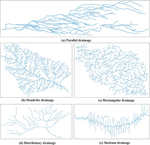
In nature, river networks are influenced by topography, climatic conditions, substratum and other factors, which shape their evolution and result in complex geometric features, diverse spatial distribution and large local differences, as shown in Table 1, which includes a number of typical drainage patterns. Drainage patterns can effectively reflect the distribution of geospatial objects and the evolution and interaction of geographic phenomena (Twidale 2004), hydrologic simulation (Jung, Marpu, and Ouarda 2017) and topographic knowledge discovery (Génevaux et al. 2013). Drainage pattern is a complex network that integrates geometric, hydrologic and geographic features of the environment, and it is challenging to identify such patterns (Zhang and Guilbert 2017). For the identification of the pattern of a river network, it is first necessary to select the indicators related to river networks, and then to establish a classification procedure. Currently, a large number of river network features have been extracted, and relevant classification rules for drainage patterns have been constructed with acceptable results (Zhang and Guilbert 2013; Jung, Shin, and Park 2019). However, the shape characteristics of river network basin units have been ignored. Due to the strict reliance on classification rules, the rich features of data samples cannot be captured, and the connection between samples cannot be effectively analysed.

Table 1. Description of typical drainage patterns.

Drainage pattern	Schematic	Specific description
Dendritic		The main and tributary streams are dendritic, which is the most common type of river networks, generally developed in sedimentary or metamorphic rock areas with consistent erosion resistance. They intersect at an acute angle pointing downstream, like a dendrite
Rectangular		The rectangular pattern is found in regions that have undergone faulting. Movements of the surface due to faulting offset the direction of the stream
Parallel		The tributaries on both sides of the main stream are more evenly distributed, nearly feathered arrangement of the river networks, long confluence time, slow flooding process after heavy rainfall, parallel or nearly parallel channels between the main stream, and tributaries
Skeleton		The tributaries are short and dense, evenly distributed on both sides of the main stream, and merge into it at approximately right angles. Mostly developed in faulted valleys or on the side of faulted cliffs, or in areas of linear folding
Distributary		Tributaries merge into the main stream from different directions, forming a fan-bone-shaped networks, this drainage pattern more concentrated at the time of confluence and prone to flooding, such as the Haihe River network^a

^a The Hai River basin is located between 112°−120°E and 35°−43°N, with two main river systems, the Hai River and the Luan River, covering an area of 317,800 square kilometres. The basin is characterised by mountains, plateaus, plains and other geomorphological forms. The river system of the Haihe river basin is fan-shaped from south to north, and as a whole is characterised by scattered secondary river networks, complex river networks, numerous tributaries, short transition zones and short and rapid river sources

When considering classification methods for drainage patterns, technology-driven and data-driven methods are widely used, especially graph neural networks in deep learning that are more advantageous, (Courtial, Touya, and Zhang 2022; Huang 2022; Yu and Chen 2022), such as for the shape of buildings recognition (Yan et al. 2021), building group patterns recognition (Yan et al. 2019; Zhao et al. 2020), road networks interchanges detection (Yang, Jiang et al. 2022). In drainage pattern recognition, pioneering studies have employed graph convolutional neural networks to construct drainage pattern classification models using an ‘end-to-end’ approach to improve the automation of drainage pattern recognition (Yu et al. 2022), although it cannot be used to effectively explore the correlated features between local river segments, and the accuracy of drainage pattern identification is limited. Therefore, there is an urgent need to construct accurate drainage pattern recognition methods.

1.1. Objectives

To address the problems of incomplete indicator for drainage pattern classification and insufficient mining of potential local correlations between river networks, this work proposes a GraphSAGE drainage pattern classification neural network method that takes into account the shape of local river basin units, which adopts supervised learning.

Firstly, typical drainage pattern samples are cut from the river networks vector database and formed into a multi-drainage pattern sample dataset through topology checking and other operations. Secondly, in order to precisely describe the morphological characteristics, taking into account the knowledge of hydrology, a system of morphological characteristics of drainage pattern is constructed from three aspects, the hierarchy of river networks, the confluence angle of river segments and the shape of local river basin units. Then, a drainage pattern classification method is constructed based on the GraphSAGE neural network, using sampling and aggregation functions to learn the neighbouring features of river segments, improve the flexible transfer of features between local river segments and to explore the potential local correlation features between river networks through inductive learning. Finally, the model is used for training and testing to achieve drainage pattern classification.

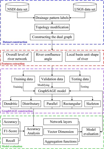
The technical route of drainage pattern recognition using GraphSAGE is shown in Figure 1. It mainly includes four parts: (1) dataset construction: construction of a multi-pattern river network sample set from different datasets; (2) feature extraction: extraction of drainage pattern features from three parts (the overall level of the river network, the confluence angle of river segments and the shape of river basin units); (3) GraphSAGE construction: construction of the GraphSAGE graph neural network for drainage pattern recognition; and (4) model evaluation: precision analysis and model evaluation.

Figure 1. Overall technical route.

1.2. Related works

The current indicators used for drainage pattern recognition mainly reflect the spatial relationships and overall basin characteristics of river networks. Among them, geometric, topological and directional indicators reflecting spatial relationships are mostly used to express the relationships between the length, curvature and connectivity of river networks (Jarvis 1976; Stanislawski 2009; Zhang and Guilbert 2013). The overall basin characteristics of river networks are mainly considered in hydrology, and the relationship between the length of the basin and its perimeter and area is reflected using indicators such as the form factor, elongation ratio and circularity ratio (Jung and Ouarda 2015; Samal, Gedam, and Nagarajan 2015; Mokarram et al. 2022). However, there is a lack of fine indicators of local basin unit characteristics to describe the pattern of the river network, which affects the accuracy of drainage pattern recognition.

Drainage pattern recognition has been extensively detailed in hydrology, geology and geomorphology (Jung, Shin, and Park 2019), influenced by the advances in computing and other technologies. The discussion has mainly focused on the conceptual level, describing the typical characteristics of different drainage patterns, the localization, their evolution and factors such as climate (Zernitz 1932; Twidale 2004). With the development of knowledge acquisition management and other techniques, the knowledge inference method has been applied to the study of drainage patterns. Primarily, statistical methods have been used to establish the inference mechanism of hierarchical identification to support classification based on the differences in relevant characteristics exhibited by distinct morphological river networks (Ichoku and Chorowicz 1994; Du, Yang, and Tan 2006; Guo and Huang 2008; Liu and Wang 2008). These methods rely on cartographic knowledge and empirical judgments of cartographic experts, which cannot be achieved by simple index inference due to differences in background knowledge and other individual aspects, increasing its difficulty.

Drainage patterns in nature are often mixed, and there are many similarities between different drainage patterns. For this reason, many studies have addressed the nonlinear problem of morphological river classification based on classifier methods and the self-similarity of river networks, using fuzzy logic, support vector machines and other techniques (Mejia and Niemann 2008; Zhang and Guilbert 2013; Jung, Shin, and Park 2019). In recent years, data-driven deep learning methods have provided new ideas for the identification problem (Reichstein et al. 2019). A related study introduced GCNs and constructed a drainage pattern recognition method based on full graph calculation that achieved good results (Yu et al. 2022), which updates the node features of the full graph in one calculation and learns that the features of the nodes are largely related to the graph structure, while the evolution of drainage patterns is strongly influenced by the local geographic environment, and it is necessary to continuously update the information of neighbouring river segments to obtain the overall features of the target river networks, which is ignored by the GCN method, resulting in insufficient mining of correlated features of river segment neighbours.

1.3. Contributions

In order to solve the problems previously described, we first use the Strahler code to encode the river network and obtain the hierarchical features of multi-pattern drainage (Strahler 1957). The convergence angle features of the river network are obtained by calculating the angle of adjacent river segments. The local basin unit of the river segment is extracted using Delaunay triangulation, and the shape features of the local basin unit are obtained using the elongation and circularity ratios to morphologically describe the river network constructed from multiple angles. Second, we take advantage of the aggregation function in the GraphSAGE network to aggregate node information from outside to inside and extract the features of the neighbours around the river segment to update the features of the target river segment. These steps allow to extract the features of locally associated river segments and increase the recognition accuracy. Finally, we build a drainage pattern recognition method based on the GraphSAGE network in PyTorch, an open source machine learning using CPU/GPU framework from the Facebook Institute for artificial intelligence that provides a flexible Python interface for easy experimentation. In this work, supervised learning is used to extract typical morphological features of river networks from typical samples, in order to improve the performance.

Overall, the paper makes two main research contributions:

1. The construction of a comprehensive and refined indicator of drainage patterns.

2. The GraphSAGE graph neural network is introduced to fully exploit the local association features of river segments for drainage pattern recognition.

The rest of this paper is organised as follows. Section 2 details the extraction and calculation of indicators related to the drainage pattern. Section 3 constructs a drainage pattern recognition method based on GraphSAGE. Section 4 presents the experimental results and detailed analysis. Section 5 discusses relevant issues, and Section 6 concludes the paper.

2. Dataset construction and data feature extraction

The GraphSAGE neural network uses supervised learning to effectively mine river morphological features and accurately recognise drainage patterns, firstly by collecting typical samples of drainage pattern in river vector databases, and secondly by combining spatial knowledge of drainage pattern to construct acceptable indicators of drainage pattern.

2.1. Dataset construction

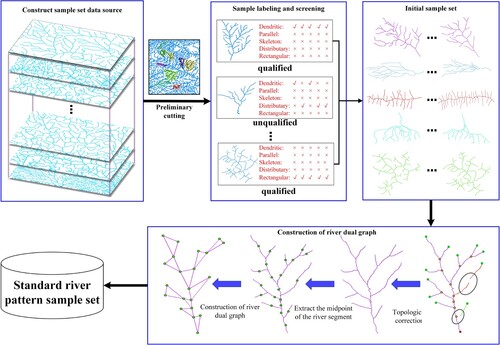
Building high-quality sample sets often improves supervised learning tasks (Du et al. 2020). In order to obtain high-quality sample datasets, multi-pattern drainage samples (dendritic, skeleton, rectangular, parallel, distributary) were collected from the USGS (USGS.gov Science for a changing world) and NSDI (http://kmap.ckcest.cn/) river network vector databases to create the sample set. The process of cropping, category labeling and filtering, and dual graph construction was then carried out. First, ten graduate students engaged in cartography were invited to crop drainage patterns from different river network vector databases, and five cartographic experts with high domain knowledge were invited to screen the preliminary sample set. Samples with different labeling results were considered unqualified, while samples with all uniform labeling results were recorded as qualified. The qualified samples were then checked for topology, such as independent river segment.

Considering that river segments provide important information about the river network, based on the data structure of the river network itself, the midpoint of the river segments was selected as the node, and the connection between the river segments was used to build the river network dual graph. Finally, each river network dual graph was regarded as a qualified sample, and multiple river network dual graphs were stored in the database to complete the construction of the qualified multiform river network sample set. In this process, G = (V, E) was defined to store river network dual graphs, where the set of nodes V = {v₁,v₂, …  … ,v_n} represent river segment objects, and E refers to the set of edges connecting the nodes. Each graph node can contain p descriptive features, forming a feature matrix F∈Rn _×p. The specific process is shown in Figure 2.

Figure 2. The process of constructing the sample set of multi-drainage pattern.

For this work, the constructed sample set contains 1750 labeled multi-drainage pattern samples, including 1000 river network samples from the NSDI database with 200 samples in each class and 750 river network samples from the USGS database with 150 samples in each class. All samples in the NSDI database and 250 samples (50 samples per class of drainage pattern) in the USGS database were used in the training and validation steps, which were randomly partitioned according to a 4:1 ratio. Thus, the training dataset had 1000 river samples, the validation dataset had 250 river samples and the remaining 500 samples in the USGS database were used as the test set.

2.2. Feature extraction for the drainage pattern

Pattern recognition consists of two basic tasks: description and classification (DeSa 2001). Given the object to be analysed, the pattern recognition system first generates a description of the object and then classifies the target object according to that description. Accurate drainage pattern description of features not only accelerate the drainage pattern recognition method convergence speed but also directly affect the effectiveness of drainage pattern recognition. Drainage patterns directly reflect the macroscopic geographic environmental characteristics of the location under analysis and may also reflect the fine local hydrologic characteristics. For this reason, this work considers four typical river network morphological indicators related to three aspects, overall river network, basin unit shape and river confluence angle, and a comprehensive and accurate drainage pattern indicator is constructed. Table 2 shows the drainage pattern description system. At the overall hierarchical level, Strahler code is used to classify the hierarchy of river networks. At the local basin level, river segments are used as the basic units of river composition, and the local basin shape is described in terms of the length, perimeter and area of the basin. Indicators of the correlation between the three are selected to reflect the rich hydrologic characteristics of the local basin. At the level of individual river segments, the angle between adjacent river segments is used to reflect their confluence, which in turn reflects the geological environment and other conditions of the local river network area.

Table 2. Drainage pattern description system.

Level	Variable	Index	Description
Overall Hierarchy	River codes	Strahler code	Hierarchical coding of river network
Local basin	River basin shape	Elongation ratio	Relationship between basin area and length
		Circularity ratio	Relationship between basin area and perimeter
Individual river segment	River confluence angle	River confluence angle	Angle of confluence between two river segments

2.2.1. Hierarchy representation of overall river network structure

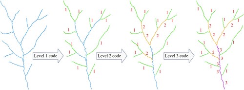
The hierarchical representation of river networks is an important tool that not only reflects the bifurcation and confluence of the river network but also measures the importance of the river in the tributary hierarchy and the evolution of the river network. Strahler coding is a typical hierarchical representation of river networks with river segments and rivers as entities, which provides the number, branching and self-similarity of river networks.

Starting from the sources of the river network, the river segments are coded as 1. When two river segments of same code intersect, the code is incremented by 1. When the codes are different, the river segment level is determined by the highest level upstream, and it increases along the river flow direction. The code of the river segment where the source is located is the smallest, and the code where the mouth is located is the largest. All the connection lines of the main stream in the river network are considered, and it is very sensitive to the addition and removal of connection lines. The specific coding process is shown in Figure 3.

Figure 3. Strahler coding process.

2.2.2. Extraction and shape quantification of local basin units in river networks

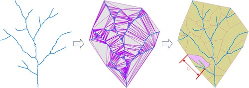
The local basin shape reflects the hydrologic characteristics of the river network, such as flow rate and sediment deposition, so it is important for drainage pattern recognition and is the main basis for identifying the drainage pattern. A basin unit is the smallest basic unit that constitutes a basin. In geographic information science, the exact location of a basin unit is usually calculated based on digital elevation model, but in vector river network data, this method is not applicable. Instead, approximations can be obtained from the river network using, for example, the convex hull.

In this work, a hierarchical partitioning method is used to delineate the boundaries of basin units (Ai, Liu, and Huang 2007), and the specific process is shown in Figure 4. The elongation ratio is proposed to reflect the relationship between the length and area of the basin unit, while the circularity ratio reflects the relationship between the area and perimeter of the basin. The quantitative calculation of the local basin unit shape allows local hydrologic information to be fully considered, which is important for the classification of drainage patterns.

Figure 4. Basin unit partitioning.

Elongation ratio: The elongation ratio (Re) is the ratio of the diameter of a circle with the same area as the basin to the maximum length of the basin (Schumm 1956), calculated according to Equation (1)(1) ${\mathrm{R}}_{\mathrm{e}}=2\sqrt{{\displaystyle \frac{\mathrm{A}}{\pi }}}/\mathrm{L}$(1) , where A is basin unit area, L is basin unit length, providing an indicator of the form of the river network that is influenced by climatic and geological factors. The closer the Re is to 1, the closer the basin shape is to a circle, and the smaller the Re is to 1, the narrower the basin tends to be. For example, the Re of the local basin of a parallel river network is smaller, which means that the local basin has a narrow shape. (1) ${\mathrm{R}}_{\mathrm{e}}=2\sqrt{{\displaystyle \frac{\mathrm{A}}{\pi }}}/\mathrm{L}$(1) Circularity ratio: The circularity ratio (Rc) is the ratio of the basin area to the area of a circle with the same perimeter as the basin perimeter (Miller 1953), calculated according to Equation (2)(2) ${\mathrm{R}}_{\mathrm{C}}={\displaystyle \frac{4\pi \mathrm{A}}{{\mathrm{P}}^2}}$(2) , where A is basin unit area, P is basin unit perimeter. It is influenced by a number of factors, including river length and frequency, topography and basin slope. If the basin has an Rc equal to 1, the basin shape is perfectly circular, and the flow is higher. The shape of basin units varies considerably in different drainage patterns, so that Rc is an acceptable indicator that reflects the circular characteristics of the local basin units. For example, the local basin shape of a rectangular pattern is close to a circle. (2) ${\mathrm{R}}_{\mathrm{C}}={\displaystyle \frac{4\pi \mathrm{A}}{{\mathrm{P}}^2}}$(2)

2.2.3. Calculation of river confluence angle

The confluence angle of a river network can be used to determine flow direction and main stream inference (Paiva and Egenhofer 2000), and it is also an important factor to consider in drainage pattern recognition (Pieri 1984). In general, a tributary merges into a main stream or two tributaries merge together to form a new main stream, forming a pinch angle at the confluence, and the variation in the confluence angle of the tributaries can be directly related to the characteristics of the river network (Hackney and Carling 2011). For example, dendritic patterns mostly occur at acute angles, while parallel patterns have smaller acute angles.

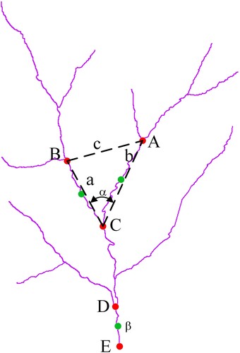
There are two types of angles involved in this work. The first is a river section not connected to the river outlet, and the confluence angle of this type of river section is calculated according to Equation (3)(3) $\alpha =\mathrm{a}\mathrm{r}\mathrm{c}\mathrm{c}\mathrm{o}\mathrm{s}\left({\displaystyle \frac{{\mathrm{a}}^2+{\mathrm{b}}^2-{\mathrm{c}}^2}{2\mathrm{a}\mathrm{b}}}\right)$(3) . The second one is a river section connected to the river outlet, and as there is only one river section, it does not constitute a confluence angle. For the sake of uniformity, we define its angle as the average confluence angle of the entire river network, calculated according to Equation (4)(4) $\text{β}={\displaystyle \frac{{}_1{+}_2{+}_3\dots {+}_{\mathrm{n}}}{\mathrm{n}}\alpha }$(4) . In Figure 5, $\alpha$ denotes the angle between river segments BC and AC, a denotes the length of river segment BC, b denotes the length of river segment AC, c denotes the distance between the upstream plotted entry points of the two river segments and $\text{β}$ denotes the angle of river segment DE. (3) $\alpha =\mathrm{a}\mathrm{r}\mathrm{c}\mathrm{c}\mathrm{o}\mathrm{s}\left({\displaystyle \frac{{\mathrm{a}}^2+{\mathrm{b}}^2-{\mathrm{c}}^2}{2\mathrm{a}\mathrm{b}}}\right)$(3) (4) $\text{β}={\displaystyle \frac{{}_1{+}_2{+}_3\dots {+}_{\mathrm{n}}}{\mathrm{n}}\alpha }$(4)

Figure 5. Example of river network confluence angle.

3. GraphSAGE neural network for drainage patterns

Machine learning algorithms have been widely used in drug discovery (Dara et al. 2021), landslide prediction (He et al. 2021), and groundwater resources survey and assessment (Ruidas et al. 2021; Pal, Ruidas et al. 2022). However, vector data does not have a neat data arrangement structure, so it is difficult to use machine learning methods for vector data research. A graph neural network is a deep learning method based on a graph structure, and vector data can be transformed into graph structured data through certain transformations, thus graph deep learning is used for the study of vector data, which can effectively process and capture relational information in graphs by passing messages between graph nodes for tasks such as classification, prediction and clustering. The essence is extracting spatial features of topological graphs, mainly in the spatial and spectral domains, and based on this feature, to be widely used in vector data processing (Yu and Chen 2022; Yang, Yuan, et al. 2022).

GCN (Kipf and Welling 2016) and GraphSAGE (Hamilton, Ying, and Leskovec 2017) are two typical types of graph neural networks. A GCN uses the entire adjacency matrix of the graph and convolutional operations to fuse the information of neighbouring nodes and is a direct inference framework in the spectral domain. GraphSAGE extracts the node neighbourhood information of the graph using neighbour sampling and aggregation functions and is an inductive spatial domain learning framework that makes it possible to represent nodes on a large graph. It is widely used in large-scale recommender systems. Considering the hierarchical neighbourhood of river networks, this work introduces the GraphSAGE neural network for use in drainage pattern recognition.

3.1. GraphSAGE neural network

GraphSAGE is a batch learning algorithm for graph nodes that transforms the transductive node representation into an inductive representation corresponding to multiple local structures, which prevents training overfitting and enhances generalisability. The core idea is to generate a feature representation of the central node by learning a representation function that aggregates on neighbouring nodes. When constructing a model using GraphSAGE, downstream tasks are accomplished mainly through neighbour sampling and information aggregation. GraphSAGE consists of mean, long short-term memory (LSTM) and maximum pooling aggregation functions, all of which are localised in space and only involve one-hop neighbours, and the aggregation function is shared among all nodes.

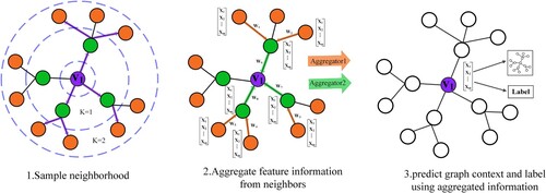
The central node uses a random sample of neighbours to select neighbours from inward to outward, which is mainly done using Equation (5)(5) ${\mathrm{N}}_{\mathrm{s}}\left({\mathrm{v}}_{\mathrm{i}}\right)=\mathrm{S}\mathrm{A}\mathrm{M}\mathrm{P}\mathrm{L}\mathrm{E}\left(\mathrm{N}\left({\mathrm{v}}_{\mathrm{i}}\right),\mathrm{S}\right)$(5) , where v_i denotes the central node, N(v_i) denotes the neighbouring nodes of the central node v_i and S denotes the number of sampled neighbouring nodes. The sample() function takes a set as input and randomly samples S elements from the input as N_s(v_i) and uses it as model input. For example, in Figure 6, three neighbours are collected in the first hop, and five are collected in the second hop. (5) ${\mathrm{N}}_{\mathrm{s}}\left({\mathrm{v}}_{\mathrm{i}}\right)=\mathrm{S}\mathrm{A}\mathrm{M}\mathrm{P}\mathrm{L}\mathrm{E}\left(\mathrm{N}\left({\mathrm{v}}_{\mathrm{i}}\right),\mathrm{S}\right)$(5) After the central node v_i samples its neighbours, the neighbours' features of the central node should be updated through the aggregation function from outside to inside based on Equation (6)(6) ${\mathrm{h}}_{\mathrm{N}\left({\mathrm{v}}_{\mathrm{i}}\right)}^{\mathrm{j}}=\mathrm{A}\mathrm{G}\mathrm{G}\mathrm{R}\mathrm{E}\mathrm{G}\mathrm{A}\mathrm{T}{\mathrm{E}}_{\mathrm{j}}\left(\left\{{\mathrm{h}}_{\mathrm{u}}^{\mathrm{j}-1},{\mathrm{\forall }}_{\mathrm{u}}\in \mathrm{N}\left({\mathrm{v}}_{\mathrm{i}}\right)\right\}\right)$(6) , where AGGREGATE_j denotes the aggregator function in layer j for aggregating information from the sampled nodes, ${\mathrm{h}}_{\mathrm{N}\left({\mathrm{v}}_{\mathrm{i}}\right)}^{\mathrm{j}}$denotes the neighbor aggregator value of node v_i at layer j, ${\mathrm{h}}_{\mathrm{u}}^{\mathrm{j}-1}$denotes the feature value of node u at layer j-1 and N(v_i) denotes the neighbours of node v_i. When j = 0, h₀ denotes the input node features. For example, in Figure 6, the neighbours features of the central node are calculated by first aggregating the features of the two-hop neighbours through aggregation function 1 to generate the node features of the one-hop neighbours. Then, the node features of the one-hop neighbours are aggregated using aggregation function 2 to complete the neighbours' features update of the central node. (6) ${\mathrm{h}}_{\mathrm{N}\left({\mathrm{v}}_{\mathrm{i}}\right)}^{\mathrm{j}}=\mathrm{A}\mathrm{G}\mathrm{G}\mathrm{R}\mathrm{E}\mathrm{G}\mathrm{A}\mathrm{T}{\mathrm{E}}_{\mathrm{j}}\left(\left\{{\mathrm{h}}_{\mathrm{u}}^{\mathrm{j}-1},{\mathrm{\forall }}_{\mathrm{u}}\in \mathrm{N}\left({\mathrm{v}}_{\mathrm{i}}\right)\right\}\right)$(6)

Figure 6. Structure of GraphSAGE.

After completing the central node v_i neighbours' features aggregation, the extracted central node features are connected with the aggregated domain neighbours node features in vector form by the concatenation operator. After this opreation, the concatenated vector is fed to the fully connected layer with the nonlinear activation function σ based on Equation (7)(7) ${\mathrm{h}}_{{\mathrm{v}}_{\mathrm{i}}}^{\mathrm{j}}=\sigma \left({\mathrm{W}}^{\mathrm{j}}\times \mathrm{C}\mathrm{o}\mathrm{n}\mathrm{c}\mathrm{a}\mathrm{t}\mathrm{e}\mathrm{n}\mathrm{a}\mathrm{t}\mathrm{e}\left({\mathrm{h}}_{{\mathrm{v}}_{\mathrm{i}}}^{\mathrm{j}-1},{\mathrm{h}}_{\mathrm{N}\left({\mathrm{v}}_{\mathrm{i}}\right)}^{\mathrm{j}}\right)\right)$(7) , thus generating the features of the central node v_i, which is used to complete the node and graph classification tasks, where W^j is a set of weight matrices for propagating information between the different layers of the model and is obtained during model training by gradient descent learning based on the loss function. (7) ${\mathrm{h}}_{{\mathrm{v}}_{\mathrm{i}}}^{\mathrm{j}}=\sigma \left({\mathrm{W}}^{\mathrm{j}}\times \mathrm{C}\mathrm{o}\mathrm{n}\mathrm{c}\mathrm{a}\mathrm{t}\mathrm{e}\mathrm{n}\mathrm{a}\mathrm{t}\mathrm{e}\left({\mathrm{h}}_{{\mathrm{v}}_{\mathrm{i}}}^{\mathrm{j}-1},{\mathrm{h}}_{\mathrm{N}\left({\mathrm{v}}_{\mathrm{i}}\right)}^{\mathrm{j}}\right)\right)$(7)

3.2. Building drainage patterns using GraphSAGE

In this work, a drainage pattern recognition method was constructed based on GraphSAGE, which is essentially an end-to-end typical graph classification network that maps the relationship between the abstract neuron space and the actual river network entity space (i.e. the description vectors of neurons correspond to the features of river network entities), and extracts the features of the graph through a series of calculations. The method consists of three main parts: data input, feature extraction and drainage pattern prediction, which are shown Figure 7.

Figure 7. Framework of GraphSAGE for drainage pattern recognition.

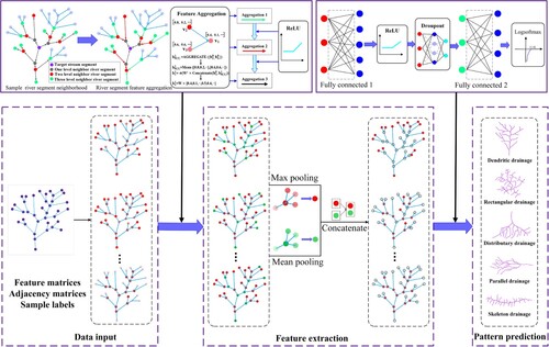
The first part of the method is the data input. The calculated drainage pattern indicators (Section 2.2) are used as the feature matrix of the dual graph. The Strahler coding of river segments and the intersection angle are normalised to maximum, and the feature matrix contains the pattern indicator description system of the river network, which is an important parameter for model learning. Based on the river segment adjacency matrix constructed in Section 2.1, the sampling function in the GraphSAGE neural network completes the sampling of river segment neighbours according to their adjacency, facilitating the flexible transfer of neighbouring river segment features. The category labels are an important reference for judging the strength of the neural network fitting ability, as the loss function calculated the difference between the forward calculation results of each iteration of the neural network and the category labels, in order to guide the next training step in the right direction.

For each river segment, the GraphSAGE neural network first completes the neighbour sampling from inside out based on its neighbouring relationship, where some of the neighbour points are randomly sampled as the target points of aggregation. The maximum number of neighbour river segments in the target river segment of the sample data set is six, and the minimum is two. The full sample method is used to complete the neighbouring sampling of each river segment, so that each river segment has sufficient surrounding neighbouring river segments. After completing the collection of neighbouring river segments, each river segment is taken as the target river segment, and the three-layer average aggregation function is used to update the characteristics of each target river segment by aggregating the information on river segments from outside to inside based on the neighbouring relationship between the segments. Finally, the characteristics of the target river segment are combined with the characteristics of the aggregated neighbouring river segments to describe the characteristics of the current river segment in vector form.

After performing information aggregation for each river segment, the ReLU activation function is used, which causes the neurons in the neural network to have sparse activation and avoids gradient explosion and gradient disappearance problems. The essence of this process involves updating the target river segment features using feature iteration from far to near, which reflects the local relevance of the first law of geography and the local geological and tectonic information about the morphological evolution of the river network. After averaging the aggregation three times, each river segment has rich feature information.

Drainage pattern recognition is a type of graph classification task, so it needs to generate graph feature information based on the node features of the graph. The proposed method introduces a pooling operation to extract feature information from river segment information in order to generate pairwise river network graphs. The pooling technique can extract the high-dimensional information of each river segment into a dense vector and then embed these node features into the generated graph features. The method uses global maximum and global mean pooling to extract the features of each river segment, in this order, and then joins the extracted information to generate the features of the river network dual graph.

The final design contains two fully connected layers, a ReLU activation layer, a droupout layer and a Log_softmax nonlinear activation layer, for drainage pattern prediction. The method uses the Adam optimiser to accelerate convergence, NLLLoss as a loss function to measure the degree of discrepancy between the output and the labels and a dropout technique to reduce overfitting. Based on the prediction results obtained from the training set, the validation set is adjusted to obtain a stable classification network structure with good prediction performance on unlabeled graphs for the purpose of drainage pattern recognition.

3.3. Experimental environment setting and important software configuration

The GraphSAGE neural network consumes a large amount of memory during training, which requires advanced hardware. The method in this paper was based on the deep learning framework PyTorch, and the deep learning experimental environment was built based on the current mainstream configuration environment. The basic configuration is given in Table 3, where the CPU contains 8 cores with parallel processing.

Table 3. Basic system platform configuration.

Operating system	CPU	Memory	Disk
Windows 10 Education	Intel Core(TM) i7-10700F CPU @ 2.90 GHz	DDR4 16 GB 3200 MHz	ST2000DM005-2CW102(2 TB)

Before the experiment, the core softwares shown in Table 4 were selected based on the computer basic system platform shown in Table 3. Python is an interpreted language, which is very convenient for writing programs; PyTorch Geometric is a PyTorch-based graph neural network base library, which provides a large number of API interfaces available for graph feature extraction; Scikit-learn was used to output the results of this method on a test set.

Table 4. Important software (package) configuration.

Graphics driver	Python	PyTorch	Scikit-learn
NVIDIA GeForce GTX 1650	3.8.5	1.8.2	0.23.2

The main components of the GraphSAGE-based drainage pattern recognition method using PyTorch Geometric mainly involve the reading in of river network dual graph (river segments adjacency, river segments features, label categories of river network dual graph), the aggregation operation and the training and testing of the method. Firstly, the input of the training set and test set of the drainage patterns are completed through the DataLoader class, in which the sampling of the river segment neighbours is performed. Secondly, the aggregation of the river segment neighbour's features and the updating of the central river segment own features are performed through the SAGEConv class. Finally, the training and testing are performed on the built method.

4. Experimental result analysis

In order to illustrate the potential of the above mentioned index system in describing drainage pattern as well as the potential of the GraphSAGE-based drainage pattern recognition neural network on mining the features of neighbouring river segments, three types of drainages that include single, mixed and multi-scale drainage patterns are selected to test this method. Then, the training process of the GraphSAGE drainage pattern recognition neural network and the test results of this method on the experimental dataset are analyzed, which proves the stability of the approach and its potential for drainage pattern recognition.

4.1. Drainage pattern classification

4.1.1. Classification of single drainage pattern

The drainage pattern recognition results achieved in this work are shown in Figure 8, which indicates that the present method provides high-quality classification performance. The target drainage patterns consist of large and small regions, and the number of river segments varies greatly in size. For regions A, B and C, which consist of multiple river segments with complex graphical structures, the method was able to accurately identify their patterns. For regions D, E, F, G, H, and I which consist of fewer river segments, the model also accurately identified their patterns.

Figure 8. Drainage pattern recognition results of single drainage pattern.

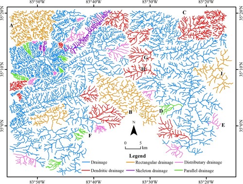
For regions G and H, most of the tributaries join the mainstream at an acute angle, and the mean values of Re and Rc for local basin units are 0.72 and 0.63, respectively. For region I, most of the tributaries join the mainstream at approximately right angles, and the mean values of Re and Rc are 0.83 and 0.73, respectively. The Re values for local basin units of the river network in region I are larger than those in regions G and H, indicating that the river basin units in region I are closer to circular than in regions G and H. The Rc value of the local river basin units in region I is larger than that in regions G and H, indicating that the local river basin units in these regions are narrower and longer than those in region I, therefore the method identified region I as a rectangular pattern and regions G and H as dendritic patterns.

In order to further verify the influence of the number of river segments in a single drainage pattern on the performance of the method, Figure 9 shows the typical drainage pattern of a large region cropped from the NSDI and USGS databases. After the method test and verification, the results are consistent with the analysis made by experts, thus demonstrating accurate pattern identification. The results show that the method can accurately identify the pattern of river segments regardless of their number. Moreover, the proposed drainage pattern index system can accurately and comprehensively describe river network patterns, improving the accuracy. Hence, the GraphSAGE neural network method constructed in this paper can identify the associations between river segments and make use of the neighbouring relationship of subsegments to flexibly transfer the features of neighbouring river segments. The pattern features of the whole river network are enhanced, and the recognition accuracy and generalisability of the method are increased.

Figure 9. Results of large regions of river network with a single pattern.

4.1.2. Classification of mixed drainage pattern

The accuracy of the proposed river network drainage pattern index and recognition were further verified by selecting river networks with multiple drainage patterns mixed together. Multi-pattern mixed river network can often be decomposed into single drainage pattern, but different people have different methods of cropping mixed drainage pattern, obtaining different cropping test data, thus reinforcing the use of the proposed method to test the drainage pattern of the cropped mixed drainage pattern. Therefore, ten graduate students that performed the dataset construction were invited to participate in the morphological identification of mixed drainage pattern.

Figure 10(a) shows the original river network, which is a typical multi-pattern mixed river network. By empirical knowledge, three of considered the area to be dendritic, and the test result of the method is a dendritic pattern. However, seven students thought that the drainage pattern needed to be further cut and divided in order to be classed, and they selected two ideal cuts. Figure 10(b,c) show two different cropping methods. In Figure 10(b), the drainage pattern was cropped according to cropping method 1, and b1 and b2 were obtained with a lower degree of cropping. After testing the pattern of the river network in b1 and b2 using the proposed method, b1 was found to have a dendritic pattern and b2 a skeleton pattern.

Figure 10. Drainage pattern recognition results of mixed drainage pattern.

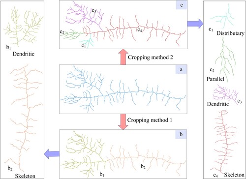
The results of c1, c2, c3 and c4 were obtained by cropping the river network using cutting method 2. Thus, the degree of cropping was higher and the results showed that c1 had a distributary pattern, c2 a parallel pattern, c3 a dendritic pattern and c4 a skeleton pattern. These results are consistent with the cartographer’s perceptions after using two different cropping methods to obtain different regional river network ranges. This indicates that the index system can accurately describe the pattern characteristics of river networks regardless of the river network selected or the target river network obtained using any cropping method. Further, the method employs the river network pattern characteristics, thus demonstrating strong recognition performance.

4.1.3. Classification of multi-scale drainage pattern

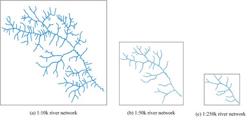
River network generalisation revealed obvious changes in the spatial relationships and number of river segments, although the pattern invariance was maintained to a certain extent. In order to verify the accurate descriptive ability of the drainage pattern indicators, multi-scale rivers were selected for the experiments. Under the condition that the river network would not be deleted after the river generalisation, river network data at three scales were selected to analyse the drainage pattern before and after the generalisation.

In Figure 11(a) is the original-scale river network at 1:10k, (b) is the river network at 1:50k scale after the 1:10k generalisation and (c) is the river network at 1:250k scale after the 1:10k generalisation. The drainage pattern at each of the three scales was tested using the proposed method, and the results all indicated a dendritic pattern, consistent with the expert results. Thus, the river network generalisation produced expected results, regardless of the changes in the original spatial relationship of the river network or the number of river segments, so the drainage pattern description index system effectively described the pattern. Further, the method can make full use of the drainage pattern characteristics of the river network and effectively exploit the association features between river segments, resulting in powerful recognition performance.

Figure 11. Multi-scale river network generalisation for drainage pattern recognition.

4.2. Analysis of the drainage pattern recognition performance

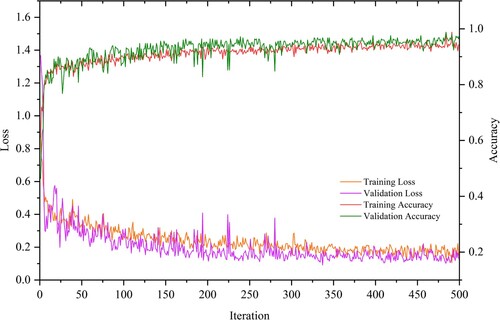
Figure 12 shows the GraphSAGE training process for the drainage pattern samples, where the accuracy of both training and validation steps is 0.9880. Based on the results, training loss and validation loss declined rapidly, whereas the accuracy of training and validation improves rapidly before 200 iterations. Training loss and validation loss declined to a small extent and the method accuracy improved by 0.08 between iterations 200 and 325. After 325 training iterations, the training loss and validation loss became stable, fluctuated slightly around 0.2, and the accuracy of the model fluctuates within a small range. All training metrics tended to be smoothly fitted. Therefore, 500 iterations were chosen for subsequent experiments to avoid overfitting.

Figure 12. Changes in training loss, validation loss, training accuracy, and validation accuracy over time.

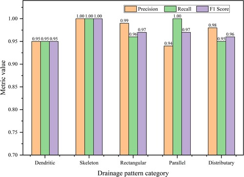
The drainage pattern recognition method constructed using GraphSAGE can efficiently identify different drainage patterns, and the results are basically the same as human perception. To further test the accuracy and generalisability of the method, 500 samples were used, where the accuracy and Kappa of the whole test set were 97.2% and 0.97, respectively. In order to evaluate the ability of the method to recognise each class of drainage pattern, three commonly used metrics were introduced: precision (P), recall (R)and F1 score (F1). In comparing the extraction results, 25 evaluation categories were considered, and several metrics were calculated directly from the confusion matrix (Table 5). (8) $\mathrm{A}={\displaystyle \frac{\mathrm{T}\mathrm{P}+\mathrm{T}\mathrm{N}}{\mathrm{T}\mathrm{P}+\mathrm{F}\mathrm{P}+\mathrm{T}\mathrm{N}+\mathrm{F}\mathrm{N}}}$(8) (9) ${\mathrm{P}}_0={\displaystyle \frac{\mathrm{T}\mathrm{P}}{\mathrm{T}\mathrm{P}+\mathrm{F}\mathrm{P}+\mathrm{T}\mathrm{N}+\mathrm{F}\mathrm{N}}}$(9) (10) ${\mathrm{P}}_{\mathrm{e}}={\displaystyle \frac{\left(\mathrm{T}\mathrm{P}+\mathrm{F}\mathrm{P}\right)\times \left(\mathrm{T}\mathrm{P}+\mathrm{F}\mathrm{N}\right)}{\left(\mathrm{T}\mathrm{P}+\mathrm{F}\mathrm{P}+\mathrm{T}\mathrm{N}+\mathrm{F}\mathrm{N}\right)\times \left(\mathrm{T}\mathrm{P}+\mathrm{F}\mathrm{P}+\mathrm{T}\mathrm{N}+\mathrm{F}\mathrm{N}\right)}}$(10) (11) $\mathrm{K}={\displaystyle \frac{{\mathrm{P}}_0-{\mathrm{P}}_{\mathrm{e}}}{1-{\mathrm{P}}_{\mathrm{e}}}}$(11) (12) $\mathrm{P}={\displaystyle \frac{\mathrm{T}\mathrm{P}}{\mathrm{T}\mathrm{P}+\mathrm{F}\mathrm{P}}}$(12) (13) $\mathrm{R}={\displaystyle \frac{\mathrm{T}\mathrm{P}}{\mathrm{T}\mathrm{P}+\mathrm{F}\mathrm{N}}}$(13) (14) $\mathrm{F}1=2\times {\displaystyle \frac{\mathrm{P}\times \mathrm{R}}{\mathrm{P}+\mathrm{R}}}$(14)

Table 5. Accuracy evaluation matrix.

Confusion matrix		Prediction
		Correct	Incorrect
Ground truth	Correct	True Positive TP	False Negative FN
	Incorrect	False Positive FP	True Negative TN

Figure 13 shows the evaluation results of the method for recognising each type of drainage pattern. The method had a high recognition accuracy of 0.9720, with an average precision of 0.9725, average recall of 0.9720 and average F1 value of 0.9720. In terms of details, most of the drainage patterns were classified into the correct categories, especially the rectangular and skeleton patterns, likely because of the obvious features of those categories. The precision for the distributary, parallel and dendritic patterns were 0.98, 0.94 and 0.95, respectively.

The proposed method can accurately identify a single drainage pattern composed of multiple river segments, a mixed drainage pattern and a multi-scale river network. The method can be used to first identify the correct pattern and then select a suitable river network generalisation method to obtain the correct generalisation results. In addition, the method can be used to evaluate the quality of the generalised river network and to measure changes in patterns before and after the generalisation, supporting automated generalisation. For mixed-pattern river networks, which are commonly found in nature, the proposed method predicts the patterns separately using different cuts of target river networks based on human empirical knowledge, and the results are consistent with the expert results.

Figure 13. Evaluation of the recognition results for each type of drainage pattern.

5. Discussion

The choice of appropriate parameters is important to increase performance. For general hyperparameters, such as learning rate and batch size, we set the learning rate to 0.008 and the batch size to 10. This structure is crucial for the ability to learn contextual information, including the searching depth with respect to the embedding vector dimension, input variables and the way GraphSAGE aggregates river segment information. The larger the neighbourhood and the greater the depth considered in GraphSAGE, the more river network information will be obtained, although it takes a long time for stability of the training step. By analysing the role of indicators related to the drainage pattern, better drainage pattern recognition methods can be obtained. In order to determine more appropriate hyperparameters, such as the number of layers and aggregation functions, a control variable approach was used in this work. Therefore, a detailed description is presented of the hyperparameter tuning, including the number of layers in the method, the dimensionality of the embedding vector, the parameter sensitivity and the selection of a better aggregator.

5.1. Parameters of GraphSAGE for recognition performance

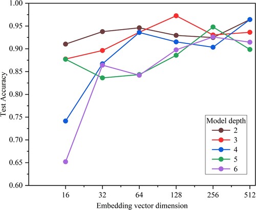
In this work, 30 sets of experiments were conducted to obtain a better combination of the number of layers and embedding vector dimensions. In these experiments, the number of layers was set to two, and the embedding vector dimensions were set to 16, 32, 64, 128, 256 and 512 in turn. The GraphSAGE model was trained and tested in order to observe its performance and to obtain the best combination of embedding vector dimensions for layer number 2. Similarly, we set the number of layers from three to six and combined them with the different embedding vectors to verify the effect of the combination of different layers with the embedding vectors.

Figure 14 shows the accuracy related to the number of network layers and embedding vector dimensions in the drainage pattern recognition results. Based on these results, the highest testing accuracy was achieved when the number of layers was set to 3 and the embedding vector to 128, so these parameters were selected in this work. There was no direct relationship between the number of layers, the embedding vector dimension size and the test accuracy, but the model accuracy was between 88.58% and 97.20% when the embedding vector dimension was set to 128, 256 and 512, so that the classification accuracy value improved.

Figure 14. Effect of the number of layers and embedding vector dimension on accuracy.

The aggregation functions in GraphSAGE have different potentials to aggregate river features for drainage pattern recognition. In this work, we conducted a series of experiments to quantitatively discover the performance of different aggregation functions in drainage pattern recognition, mainly LSTM, maximum pooling and the mean aggregation function. Table 6 shows the experimental results after aggregation using different aggregation operators. LSTM, maximum pooling and mean aggregation functions all showed high training performance, which indicates the powerful information aggregation potential of the GraphSAGE neural network. There were small differences between the different aggregation functions, for example, mean aggregation focuses on the average level of river segment features, while the maximum pooling operation focuses on the maximum value of a feature in a river segment. The mean aggregation function has low computational complexity and exhibited high performance in terms of test accuracy and computation time, and thus it was used in this work.

Table 6. Impact of different aggregation functions on model performance.

Aggregation function	Training accuracy	Testing accuracy	Training time (s)
LSTM	0.9691	0.9543	587.67
Maximum Pooling	0.9752	0.9431	360.15
Mean	0.9882	0.9720	356.95

5.2. Performance of design features in drainage pattern recognition

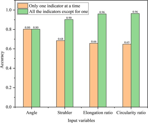
Figure 15 shows a comparison of the recognition results using only one descriptive indicator at a time or all but one indicator as input variables to investigate the impact of the input variables on recognition performance. The accuracy reached 97.2% when four indicators were used as input variables and was lower than 97.2% when any single indicator was missing, suggesting that each indicator plays a role in the classification of river networks. When one indicator was used as an input variable, the river network convergence angle indicator had the greatest influence on drainage pattern recognition, followed by the Strahler code of the river network, while the Re and Rc had a smaller influence. On the one hand, this finding further highlights the impact of geomorphology on the river networks and the importance of the confluence angle and the Strahler code in drainage pattern recognition. On the other hand, it could be attributed to the extraction of local basin units of river networks, which is a complex and difficult process to quantify.

Figure 15. Effect of different input variables on recognition performance.

Figure 16 shows the degree of influence of the features on different drainage patterns, illustrating the importance of different features for improving performance. Different classification metrics were used for each type of pattern in order to assess the performance of each class of features on drainage pattern recognition. From these results, when using the Re and Rc, a rectangular pattern could be accurately recognised, and the accuracy was also high for the parallel pattern. This indicates that the shapes of the basin units in the rectangular and parallel patterns are distinct. The basin units in the rectangular pattern are square and nearly square, while the shape of the basin units in the parallel pattern are distinctly narrow.

Figure 16. Effect of a single indicator on drainage pattern recognition performance.

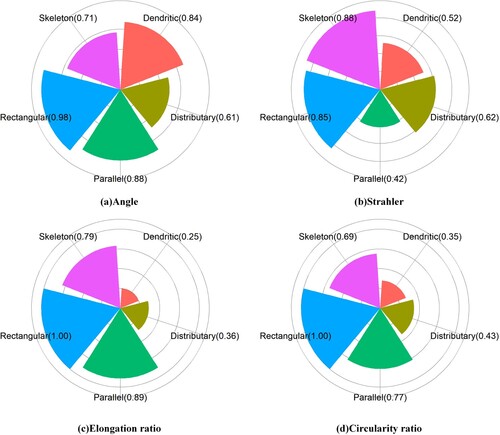
Meanwhile, in the other three categories, the performance of this indicator was average, which can be attributed to the fact that these types of river basin units do not have obvious shape characteristics. This result is consistent with the characteristics of the actual river network. The average accuracy of the angle indicator was high for each drainage pattern, especially the rectangular pattern and also for the dendritic and parallel patterns, mainly due to the fact that the rectangular pattern includes approximately right angles, the parallel pattern has smaller acute angles and the dendritic pattern has larger acute angles. The Strahler code showed the best skeleton pattern recognition performance, mainly due to the low fractality of the skeleton pattern.

Table 7 shows the combination of other indicators. The shape of the basin unit along with the river network’s confluence angle and Strahler code were features learned by the method to obtain a mutual replacement or complementary indicators for the proposed method. Among the three types of indicators, only one is involved at the river network level. Therefore, in this work, the confluence angle of river segments and the Strahler code of the river network were used as fixed input variables in the model. Form factor and the lemniscate ratio were selected to determine the relationship between axis length and area in the shape of river network local basin unit, while the compactness constant and fractal dimension were selected to reflect the relationship between perimeter and area in the shape of the river network.

Table 7. Replacement or supplementary indicators for the proposed method.

Set	Angle	Strahler	Form Factor	Lemniscate ratio	Compactness Constant	Fractal Dimension	Test Accuracy
1	√	√	√		√		0.9451
2	√	√	√			√	0.9700
3	√	√		√	√		0.9486
4	√	√		√		√	0.9689

With the other parameters being the same, the abovementioned factors were combined as input variables and tested separately. Table 7 shows the input variables and recognition results from the four sets of experiments. The test accuracies were above 94% and up to 97%, indicating that the use of these four indicators had high accuracy and could replace or supplement the indicators chosen for the proposed method.

5.3. Comparative analysis

In this work, the proposed method was compared with other machine learning methods, including GCN, graph attention network (GAT), random forest (RF) and support vector machine (SVM), using the same datasets (training, validation and testing datasets) to demonstrate that the proposed method can learn deep features of river networks with strong recognition performance. Figure 17 shows the potential results of the proposed GraphSAGE-based drainage pattern recognition method for the classification of drainage patterns. The GraphSAGE neural network uses the aggregation function to extract river segment features, which greatly benefits from the typical contextual information of local river segments. In addition, the method can learn more river features to classify drainage patterns.

Figure 17. Comparison between accuracy results from different machine learning methods.

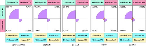
GAT aggregates neighbouring nodes through an attention mechanism, which adaptively assigns weights according to the importance of the neighbours. However, it is overly sensitive to some features, resulting in larger weight assignments, thus exhibiting poor performance. GraphSAGE is an information transfer framework, and through the aggregation function, a node is able to aggregate information about its neighbours and update the information of the current node through an update function, which is an iterative information transfer process. Both GCN and GAT can only obtain first-order neighbourhoods, while GraphSAGE can learn from more neighbourhood information as the number of layers increases. RF and SVM perform poorly compared to traditional machine learning methods because they cannot mine the river network for deeper river network features.

Both the method in this work and GCN method (Yu et al. 2022) use graph deep learning techniques to achieve drainage pattern recognition with a data-driven supervised learning method. Compared with traditional rule-based and other methods, the data-driven approach can obtain better learning parameters, effectively identify the geomorphology of the data when its scale or geographic features change, and has a strong self-adaptive capability, with high recognition accuracy and automation level. Compared with the GCN method, the method in this work is convenient and flexible in sampling river segments during training, and can fully exploit the associated features of neighbouring river segments, and is also a neural network method for drainage pattern recognition that takes into account features such as geological formations.

6. Conclusions

The proposed drainage pattern recognition method based on the GraphSAGE neural network, which considers the local basin unit shape features of river networks, was applied it to single drainage, mixed drainage and multi-scale drainage pattern recognition tasks. First, a high-quality typical sample data set was constructed from the NSDI and USGS river network databases. Second, for the typical drainage pattern sample set, four typical drainage pattern indicators were extracted based on three factors – the overall level of the river network, the confluence angle of river segments and the shape of river basin units – which reflect the hydrology, geometry and shape of river basin units to achieve a comprehensive and accurate description of river networks. The proposed method also aggregates the neighbouring features of the river network through an aggregation function to explore the association features of the river network. Finally, by controlling the searching depth and embedding vector dimensions, different aggregation functions and other parameters, we compared the potential of the method to mine river network association features with different parameter combinations.

In the test dataset, the overall accuracy reached 97.2%, and it was especially accurate in identifying skeleton and rectangular patterns. The method was also tested on a large range of single-pattern, mixed-pattern and multi-scale river network data. It accurately identified drainage pattern types, and the recognition results were consistent with the results from empirical knowledge by experts, indicating that the drainage patterns index proposed in this work is not affected by the number of river segments and can flexibly and accurately describe their patterns. Further, the drainage pattern method constructed based on the GraphSAGE neural network has a strong ability to mine the correlation characteristics between river segments. The results of this work were obtained by analysing deep drainage patterns, not by simply weighting elements for calculation, thus providing a comprehensive and objective assessment. Therefore, the proposed method can be used by hydrology researchers for accurate modelling of regional hydrological information, by emergency management authorities for rational and effective enhancement of flood management, and by map research authorities for improved automation of river networks generalisation.

The method also has some limitations. The river networks in this work were obtained by manual segmentation, which is not conducive to the automatic generalisation of river networks. Future research should use the basin characteristics, such as the shape of river basin units, to collect river segments with similar characteristics. Clustering methods could then be employed to support automatic morphological segmentation of river networks and improve the automation of river generalisation.

Acknowledgements

The authors would like to express special thanks to editor and all the anonymous reviewers for their valuable comments that helped improve the manuscript.

Disclosure statement

No potential conflict of interest was reported by the author(s).

Data availability statement

If readers need data or code, please contact us by email.

Additional information

Funding

This work was supported by the National Natural Science Foundation of China [grant number 41930101,42161066, 42261076]; State Key Laboratory of Geo-Information Engineering and Key Laboratory of Surveying and Mapping Science and Geospatial Information Technology of MNR, CASM [grant number 2022-03-03]; Major Project for Science and Technology of Gansu Province [grant number 22ZD6GA010]; Youth Science and Technology Foundation of Gansu Province [grant number 22JR11RA140]; Young Scholars Science Foundation of Lanzhou Jiaotong University [grant number 2022007].

References

- Ai, Tinghua, Yaolin Liu, and Yafeng Huang. 2007. “The Hierarchical Watershed Partitioning and Generalisation of River Network.” Acta Geodaetica et Cartographica Sinica 36 (2): 231–236 + 243.
- Brassel, Kurt E, and Robert Weibel. 1988. “A Review and Conceptual Framework of Automated Map Generalisation.” International Journal of Geographical Information Systems 2 (3): 229–244. doi:10.1080/02693798808927898.
- Courtial, Azelle, Guillaume Touya, and Xiang Zhang. 2022. “Constraint-Based Evaluation of Map Images Generalized by Deep Learning.” Journal of Geovisualization and Spatial Analysis 6 (1): 1–17. doi:10.1007/s41651-021-00095-6.
- Dara, Suresh, Swetha Dhamercherla, Surender Singh Jadav, CH Madhu Babu, and Mohamed Jawed Ahsan. 2021. “Machine Learning in Drug Discovery: A Review.” Artificial Intelligence Review 55: 1947–1999. doi:10.1007/s10462-021-10058-4.
- De Sa, JP Marques. 2001. Pattern Recognition: Concepts, Methods and Applications. Berlin: Springer Science & Business Media.
- Du, Peijun, Xuyu Bai, Kun Tan, Zhaohui Xue, Alim Samat, Junshi Xia, Erzhu Li, Hongjun Su, and Wei Liu. 2020. “Advances of Four Machine Learning Methods for Spatial Data Handling: a Review.” Journal of Geovisualization and Spatial Analysis 4 (1): 1–25. doi:10.1007/s41651-019-0044-z.
- Du, Qingyun, Pinfu Yang, and Renchun Tan. 2006. “Classification of River Networks Structure Based on Spatial Statistical Character.” Geomatics and Information Science of Wuhan University 31 (5): 419–422.
- Génevaux, Jean-David, Éric Galin, Eric Guérin, Adrien Peytavie, and Bedrich Beneš. 2013. “Terrain Generation Using Procedural Models Based on Hydrology.” ACM Transactions on Graphics 32 (4): 1–13.
- Guo, Qingsheng, and Yuanlin Huang. 2008. “Automatic Reasoning on Main Streams of Tree River Networks.” Geomatics and Information Science of Wuhan University 33 (9): 978–981.
- Hackney, Christopher, and Paul Carling. 2011. “The Occurrence of Obtuse Junction Angles and Changes in Channel Width Below Tributaries Along the Mekong River, South-East Asia.” Earth Surface Processes and Landforms 36 (12): 1563–1576. doi:10.1002/esp.2165.
- Hamilton, Will, Zhitao Ying, and Jure Leskovec. 2017. “Inductive Representation Learning on Large Graphs.” Advances in Neural Information Processing Systems 30.
- He, Yi, Zhanao Zhao, Wang Yang, Haowen Yan, Wenhui Wang, Sheng Yao, Lifeng Zhang, and Tao Liu. 2021. “A Unified Network of Information Considering Superimposed Landslide Factors Sequence and Pixel Spatial Neighbourhood for Landslide Susceptibility Mapping.” International Journal of Applied Earth Observation and Geoinformation 104: 102508. doi:10.1016/j.jag.2021.102508.
- Huang, Wei. 2022. “What were GIScience Scholars Interested in During the Past Decades?.” Journal of Geovisualization and Spatial Analysis 6 (1): 1–21. doi:10.1007/s41651-021-00095-6.
- Ichoku, Charles, and Jean Chorowicz. 1994. “A Numerical Approach to the Analysis and Classification of Channel Network Patterns.” Water Resources Research 30 (2): 161–174. doi:10.1029/93WR02279.
- Jarvis, Richard S. 1976. “Classification of Nested Tributary Basins in Analysis of Drainage Basin Shape.” Water Resources Research 12 (6): 1151–1164. doi:10.1029/WR012i006p01151.
- Jiang, Lili, Qingwen Qi, and An Zhang. 2015. “River Classification and River Network Structuration in River Auto-Selection.” Geomatics and Information Science of Wuhan University 40 (6): 841–846.
- Jung, Kichul, Prashanth R. Marpu, and Taha BMJ Ouarda. 2017. “Impact of River Network Type on the Time of Concentration.” Arabian Journal of Geosciences 10 (24): 1–17.
- Jung, Kichul, and Taha B. M. J. Ouarda. 2015. “Analysis and Classification of Channel Network Types for Intermittent Streams in the United Arab Emirates and Oman.” Journal of Civil & Environmental Engineering 5 (5): 159–218.
- Jung, Kichul, Juyong Shin, and Daeryong Park. 2019. “A New Approach for River Network Classification Based on the Beta Distribution of Tributary Junction Angles.” Journal of Hydrology 572: 66–74. doi:10.1016/j.jhydrol.2019.02.041.
- Kipf, Thomas N, and Max Welling. 2016. “Semi-Supervised Classification with Graph Convolutional Networks.” arXiv preprint arXiv:1609.02907.
- Liu, Huai xiang, and Zhaoyin Wang. 2008. “Relationship Between River Network Pattern and Environmental Condition.” Journal of Tsinghua University (Science and Technology) 48 (9): 1408–1412.
- Mejía, Aifonso I, and Jeffrey D Niemann. 2008. “Identification and Characterization of Dendritic, Parallel, Pinnate, Rectangular, and Trellis Networks Based on Deviations from Planform Self-Similarity.” Journal of Geophysical Research Earth Surface 113: 1–12.
- Miller, V. C. 1953. A Quantitative Geomorphologic Study of Drainage Basin Characteristics in the Clinch Mountain Area, Virginia and Tennessee. Project NR 389042, Tech Report, Columbia University Department of Geology, ONR Geography Branch, New York. Retrieved from http://agris.fao.org/agris-search/search.do? recordID = US201400058936
- Mokarram, Marzieh, Hamid Reza Pourghasemi, John P. Tiefenbacher, and Ali Saber. 2022. “Prediction of Drainage Morphometry Using a Genetic Landscape Evolution Algorithm.” Geocarto International 37 (5): 1364–1377. doi:10.1080/10106049.2020.1762766.
- Paiva, Joo Argemiro Cavalho, and Max J Egenhofer. 2000. “Robust Inference of the Flow Direction in River Networks.” Algorithmica 26 (2): 315–333.
- Pal, Subodh Chandra, Indrajit Chowdhuri, Biswajit Das, Rabin Chakrabortty, Paramita Roy, Asish Saha, and Manisa Shit. 2022. “Threats of Climate Change and Land Use Patterns Enhance the Susceptibility of Future Floods in India.” Journal of Environmental Management 305: 114317.
- Pal, Subodh Chandra, Dipankar Ruidas, Asish Saha, Abu Reza Md. Towfiqul Islam, and Indrajit Chowdhuri. 2022. “Application of Novel Data-Mining Technique-Based Nitrate Concentration Susceptibility Prediction Approach for Coastal Aquifers in India.” Journal of Cleaner Production 131205.
- Pieri, David C. 1984. “Junction Angles in Drainage Networks.” Journal of Geophysical Research Solid Earth 89 (B8): 6878–6884. doi:10.1029/JB089iB08p06878.
- Reichstein, Markus, Gustau Camps-Valls, Bjorn Stevens, Martin Jung, Joachim Denzler, Nuno Carvalhais, and Prabhat. 2019. “Deep Learning and Process Understanding for Data-Driven Earth System Science.” Nature 566 (7743): 195–204. doi:10.1038/s41586-019-0912-1.
- Ruidas, Dipankar, Rabin Chakrabortty, Abu Reza Md. Towfiqul Islam, Asish Saha, and Subodh Chandra Pal. 2022. “A Novel Hybrid of Meta-Optimization Approach for Flash Flood-Susceptibility Assessment in a Monsoon-Dominated Watershed, Eastern India.” Environmental Earth Sciences 81 (5): 1–22.
- Ruidas, Dipankar, Subodh Chandra Pal, Abu Reza Md. Towfiqul Islam, and Asish Saha. 2021. “Characterization of Groundwater Potential Zones in Water-Scarce Hardrock Regions Using Data Driven Model.” Environmental Earth Sciences 80 (24): 1–18.
- Samal, Dipak R, Shirish S Gedam, and R. Nagarajan. 2015. “GIS Based Drainage Morphometry and its Influence on Hydrology in parts of Western Ghats region, Maharashtra, India.” Geocarto International 30 (7): 755–778. doi:10.1080/10106049.2014.978903.
- Schumm, Stanley A. 1956. “Evolution of Drainage Systems and Slopes in Badlands at Perth Amboy, New Jersey.” Geological Society of America Bulletin 67 (5): 597–646. doi:10.1130/0016-7606(1956)67[597:EODSAS]2.0.CO;2.
- Stanislawski, Lawrence V. 2009. “Feature Pruning by Upstream Drainage Area to Support Automated Generalisation of the United States National Hydrography Dataset.” Computers, Environment and Urban Systems 33 (5): 325–333. doi:10.1016/j.compenvurbsys.2009.07.004.
- Strahler, Arthur N. 1957. “Quantitative Analysis of Watershed Geomorphology.” Eos, Transactions American Geophysical Union 38 (6): 913–920. doi:10.1029/TR038i006p00913.
- Twidale, C. R. 2004. “River Patterns and Their Meaning.” Earth Science Reviews 67 (3-4): 159–218. doi:10.1016/j.earscirev.2004.03.001.
- Wang, Jiayao, Zhilin Li, and Fang Wu. 2011. Advances in Digital Map Generalisation. Beijing: Science Press.
- Wang, Jiayao, Qun Sun, Guangxia Wang, Jiang Nan, and Xiaohua lv. 2014. Principle and Methods of Cartography. 2nd ed. Beijing: Science Press.
- Yan, Xiongfeng, Tinghua Ai, Min Yang, and Xiaohua Tong. 2021. “Graph Convolutional Autoencoder Model for the Shape Coding and Cognition of Buildings in Maps.” International Journal of Geographical Information Science 35 (3): 490–512. doi:10.1080/13658816.2020.1768260.
- Yan, Xiongfeng, Tinghua Ai, Min Yang, and Hongmei Yin. 2019. “A Graph Convolutional Neural Network for Classification of Building Patterns Using Spatial Vector Data.” ISPRS Journal of Photogrammetry and Remote Sensing 150 (4): 259–273.
- Yang, Min, Chenjun Jiang, Xiongfeng Yan, Tinghua Ai, Minjun Gao, and Wenyuan Chen. 2022. “Detecting Interchanges in Road Networks Using a Graph Convolutional Network Approach.” International Journal of Geographical Information Science 36 (6): 1119–1139. doi:10.1080/13658816.2021.2024195.
- Yang, Min, Tuo Yuan, Xiongfeng Yan, Tinghua Ai, and Junjiang Chen. 2022. “A Hybrid Approach to Building Simplification with an Evaluator from a Backpropagation Neural Network.” International Journal of Geographical Information Science 36 (2): 280–309. doi:10.1080/13658816.2021.1873998.
- Yu, Huafei, Tinghua Ai, Min Yang, Lina Huang, and Jiaming Yuan. 2022. “A Recognition Method for Drainage Patterns Using a Graph Convolutional Network.” International Journal of Applied Earth Observations and Geoinformation 107: Article 102696. doi:10.1016/j.jag.2022.102696.
- Yu, Wenhao, and Yujie Chen. 2022. “Data-driven Polyline Simplification Using a Stacked Autoencoder-based Deep Neural Network.” Transactions in GIS 26 (5): 2302–2325. doi:10.1111/tgis.12965.
- Zernitz, Emilie R. 1932. “Drainage Patterns and Their Significance.” The Journal of Geology 40 (6): 498–521. doi:10.1086/623976.
- Zhang, Ling, and Eric Guilbert. 2013. “Automatic Drainage Pattern Recognition in River Networks.” International Journal of Geographical Information Science 27 (12): 2319–2342. doi:10.1080/13658816.2013.802794.
- Zhang, Ling, and Eric Guilbert. 2017. “A Genetic Algorithm for Tributary Selection with Consideration of Multiple Factors.” Transactions in Gis 21 (2): 332–358. doi:10.1111/tgis.12205.
- Zhao, Rong, Tinghua Ai, Wenhao Yu, Yakun He, and Yilang Shen. 2020. “Recognition of Building Group Patterns Using Graph Convolutional Network.” Cartography and Geographic Information Science 47 (5): 400–417. doi:10.1080/15230406.2020.1757512.
- Zhu, Guorui, Lizhen Guo, Gongbai Yin, and Yongli Xu. 2001. Map Design and Compilation. 2nd ed. Wuhan: Wuhan university press.