Estimating PM_2.5 concentrations in a central region of China using a three-stage model

ABSTRACT

Owing to uneven environmental monitoring site distribution, there are significant spatial data gaps for concentrations of ambient fine particles with diameters ≤ 2.5 µm (PM_2.5) obtained using traditional monitoring methods. Satellite products are an alternative data source for locations where monitoring sites are unavailable. The Moderate Resolution Imaging Spectroradiometer (MODIS) aerosol optical depth (AOD) product has been widely used in PM_2.5 assessment for years; however, it has obvious data gaps in winter. Here, the Visible Infrared Imaging Radiometer Suite (VIIRS) AOD was applied to supplement MODIS AOD data to obtain a fused AOD dataset. A three-stage model consisting of a corrected AOD model, mixed effects model, and geographically weighted regression model was developed and used with meteorological and vegetation factors to estimate PM_2.5. Results showed overall model fitting by cross-validation (CV) with an R² of 0.92, mean absolute error of 5.72 µg/m³, and root mean square error of 7.15 µg/m³. The combination of MODIS AOD and VIIRS AOD was a suitable method for enhancing AOD coverage. The CV R² value of the three-stage model (0.92) was higher than that of the two-stage model (0.9). Hence, the three-stage model could achieve a better fit in estimating PM_2.5 on a regional scale.

KEYWORDS:

• VIIRS AOD
• MODIS AOD
• PM_2.5 concentrations
• combined model

1. Introduction

Ambient fine particles with diameters ≤ 2.5 µm (PM_2.5) can reach the alveolar area through the respiratory system and cause damage to the human body (Sun et al. 2020). Exposure to PM_2.5 over a long period increases the incidence of lung cancer and cardiovascular diseases (Sun et al. 2020). Global disease burden data indicate that China has the world’s third largest risk factor for premature death which is atmospheric PM_2.5, with 2 million deaths in China every year due to air pollution (Wang et al. 2021). To determine PM_2.5 levels, the PM_2.5 concentrations in different areas must be known, and the distribution of these concentrations can be obtained by interpolating station measurements. However, because of the large spatial distances between stations, a surface environmental monitoring network is inadequate for capturing the spatial changes in PM_2.5 concentrations, which can seriously affect the accuracy of PM_2.5 health risk assessments (Hu et al. 2014). However, satellite-based remote sensing can simultaneously achieve high spatial resolution and spatial coverage. It is a good alternative tool because of the lack of ground-based environmental monitoring. Aerosol optical depth (AOD) is an essential factor in the measurement of atmospheric aerosol levels, and it can be used to characterize atmospheric turbidity or the total aerosol concentration (Liu et al. 2015).

Previous studies have focused on the relationship between AOD and PM_2.5. Clear positive correlations have been reported in most regions (Gupta et al. 2006; Natunen et al. 2010). The AOD-PM_2.5 relationship has a weak correlation in a few areas (Engel-Cox et al. 2004; Jin et al. 2021), such as the western United States and the summer and autumn in Beijing. Wang et al. (2010), Chen et al. (2014), and Jin et al. (2021) proved that the relationship between AOD and PM_2.5 was significantly improved by vertical and relative humidity (RH) adjustment. Zhang et al. (2021) developed a physical processes model to explain the AOD-PM_2.5 relationship, and the results demonstrated that physical processes, such as vertical distribution and hygroscopic growth function, are very important factors in the study of the relationship between AOD and PM_2.5. In this study, a vertical-and-RH correction was added for AOD to test whether the fit of the model could be further enhanced.

Methods of obtaining AOD data that simulate ground-level PM_2.5 concentrations have rapidly developed in recent years. A number of statistical and machine learning methods have been applied for this purpose, such as back propagation neural networks (Guo et al. 2013), Bayesian-based statistical models (Lv et al. 2016; Lv et al. 2017), land-use regression models (Wu, Xie, and Li 2016; Xu et al. 2016), geographically weighted regression (GWR) models (Chen et al. 2016; Karimian et al. 2017), Bayesian geostatistical models (Beloconi et al. 2018), random forest models (Chen et al. 2019), and machine learning (Schneider et al. 2020). These models have higher R² values than a simple regression model. However, they also have some deficiencies; for example, temporal variations have not been sufficiently considered, which can affect the estimation accuracy. Due to the differences in the satellite inversion environment and daily meteorological conditions, there are more temporal variations than spatial variations in the relationship between AOD and PM_2.5 (Jing et al. 2018). Lee et al. (2011) first established the mixed effects (LME) model to simulate PM_2.5 concentrations in the northeast of the USA and achieved a model R² value of 0.97, which proved that the LME model had good simulation ability by considering time variables. Xie et al. (2015) and Hu et al. (2014) utilized LME to explain the daily AOD-PM_2.5 relationship and obtained a high model fit in China. Ma et al. (2016a) established a two-stage model by combining the LME model with the generalized additive model (GAM) to explain the spatio-temporal relationships of AOD-PM_2.5. He and Huang (2018a, 2018b) developed a geographically and temporally weighted regression to simulate PM_2.5, which had the advantage of spatial relationships of GWR because of its capacity to resolve spatial variation. The LME model performed better in terms of temporal estimation, whereas GWR was a better spatial model than the GAM. In the present study, the advantages of each model were combined to develop a more accurate model (three-stage model) to estimate PM_2.5 concentrations in Fenwei.

Spatial gaps in winter PM_2.5 estimates due to gaps in the AOD data have been observed. Therefore, it is necessary to develop a suitable method for reducing these gaps. Several studies have used model data to resolve this problem (Ma et al. 2016a; Hoogh et al. 2018; Chen et al. 2020; Li et al. 2020a), and others have used multiple data fusion techniques to fill AOD gaps (Donkelaar et al. 2015; Chen et al. 2016; Handschuh et al. 2022). Remarkably, when a model simulation is used to fill in the missing data, insufficient calculations may lead to deviations (Yang, Xu, and Jin 2018). Therefore, it is important to use multi-sensor data fusion instead of model data to fill these gaps. Moderate Resolution Imaging Spectroradiometer (MODIS) AOD products (Collection 6.1) have been proven to be suitable for simulating PM_2.5 concentrations in different regions of China (Ma et al. 2016a, 2016b; Jing et al. 2018). Compared with the 10 km product, a 3 km resolution was identified as an appropriate scale for estimating PM_2.5 concentration distributions in cities (Yang et al. 2020). Nevertheless, MODIS 3 km AOD has poor retrieval in bright urban surfaces and heavy pollution areas in winter (Munchak et al. 2013). Yao et al. (2018) reported that the spatio-temporal coverage of Visible Infrared Imaging Radiometer Suite (VIIRS) AOD was substantially improved, especially in winter. Combining the advantages of VIIRS AOD and MODIS AOD to fill the spatial gap represents an effective data fusion method that can provide a reference for other studies.

In this study, the application of VIIRS AOD and MODIS AOD to the Fenwei Plain was investigated. Considering the physical significance of AOD and the spatio-temporal variability of AOD-PM_2.5, a three-stage model was developed. First, planetary boundary layer height (PBLH) and RH were used to establish a vertical-and-RH correction of the AOD. Second, an LME was utilized to explore temporal variation. Third, a GWR was established to explain spatial variation. Cross-validation (CV) was utilized to check the accuracy of the three-stage model. Finally, the monthly, seasonal, and annual PM_2.5 concentrations were estimated for the Fenwei Plain in 2018. The results of this study also provided basic data support for PM_2.5 health risk assessments and air pollution control.

2. Data and methodology

2.1. Study region

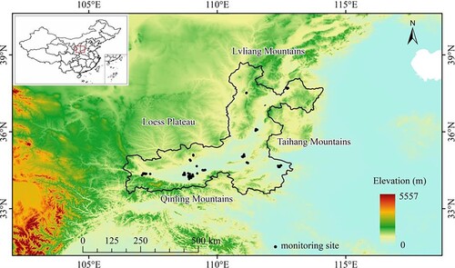
The Fenwei Plain, located in the central region of China, has severe air pollution (33.5°N–38.7°N, 106.3°E–114.2°E), including in the Weihe Plain, Fenhe Plain, and surrounding terraces. The average elevation of the Fenwei Plain is approximately 500 m (Figure 1). The Fenwei Plain is surrounded by the Tai-hang Mountains to the east, Qin-ling Mountains to the south, and Loess Plateau to the west and north. Pollutant dispersion is prohibited because of the narrow area from the northeast to the southwest. The Fenwei Plain contains 12 cities in three different provinces, most of which are located in river valleys. The Fenwei Plain is also adjacent to the seriously polluted Beijing-Tianjin-Hebei-Shandong region and is often affected by the transmission of pollution from the east. The region is also affected by sand and floating dust from the northwest arid area during spring and autumn. The unique geographic location and complex topographic conditions of the study area have made estimation challenging. Therefore, the development of successful assessment methods to estimate PM_2.5 concentrations in this location will be of great value to this field of research.

Figure 1. Elevation of the study area and location of environmental monitoring sites.

2.2. Data

2.2.1. The MODIS AOD

The MODIS sensor was carried on the Terra and Aqua satellites, which were launched on 18 December 1999, and 4 May 2002, respectively. The overpass times were 10:30 am and 13:30 pm local time, respectively. The temporal resolution of the MODIS sensor is 1 day, and it can acquire observations of 36 bands, which provides full spectral coverage from 0.4 to 14.4 µm. The 3 km product is very similar to the 10 km product, but there are some differences in obtaining reflectivity and spatial resolution (Remer et al. 2013). Two-thirds of the MODIS 3 km AOD released by NASA in 2014 are within the allowable error range and can be used for global aerosol research (Munchak et al. 2013). Compared with the deep blue (DB) and merged dark target (DT) and DB algorithms, the DT algorithm is more suitable for urban, grassland, and forest areas (Li et al. 2020b). Therefore, considering the land use type of the research area in the present study, a DT AOD of 550 nm was chosen for land with higher quality (quality flag = 2, 3). MOD04_3 K and MYD04_3 K data from the Terra and Aqua satellites were provided by NASA (https://ladsweb.modaps.eosdis.nasa.gov). After de-clouding with masking techniques, 1,461 images were collected from the Fenwei Plain in 2018 (1 January to 31 December).

MODIS AOD images were preprocessed using ENVI® image analysis software. First, geometric corrections and projective transformations were processed using the MODIS Conversion Toolkit, then multiple images of the area were spliced into one using a seamless mosaic. Finally, 346 Terra AOD images and 360 Aqua AOD images were obtained for 2018.

2.2.2. The VIIRS AOD

VIIRS is a sensor mounted on the National Polar-orbiting Operational Environmental Satellite System Preparatory Pro (NPP). The overpass time of the NPP satellite was 13:30 pm locally. The instrument performance and bands of the VIIRS were adjusted and improved to be above those of the MODIS (Bian et al. 2018). The AOD inversion algorithm of the VIIRS is similar to the MODIS DT algorithm, but it differs in terms of spectral bandwidth, wavelengths, and calibration algorithms (Jackson et al. 2013; Choi et al. 2019). The VIIRS can generate a set of aerosol parameters (including 550 nm AOD) (Liu et al. 2014). The 6 km AOD product was released by the VIIRS aerosol team after the data were further processed (Jackson et al. 2013). This dataset contained four types of data quality products: none, low-quality, medium-quality, and high-quality data (quality flag = 0, 1, 2, and 3). Yao et al. (2018) showed that medium-quality data could not only meet the estimation accuracy of PM_2.5, but also ensure sufficient spatial coverage in China. In this study, a 6 km AOD at 550 nm with medium-quality data was chosen. The daily product was downloaded from NOAA (www.class.noaa.gov/) and a total of 100 NetCDF(.nc) files were collected.

First, the latitude, longitude, and AOD values were extracted into a point file using MATLAB. Second, the points to raster were converted using ArcGIS®. Third, the 6 km VIIRS AOD was resampled to 3 km.

2.2.3. Monitoring of PM_2.5

Monitoring data of PM_2.5 were provided by the Chinese National Environmental Monitoring Center (http://www.cnemc.cn/). PM_2.5 samples were monitored using β-ray methods or TEOM, with total quality control implemented for the automatic monitoring equipment to ensure the quality of the data. Environmental data were collected from 62 environmental monitoring sites on the Fenwei Plain (Figure 1). Daily average PM_2.5 concentrations were utilized to match the daily AOD data from 1 January to 31 December 2018.

2.2.4. Meteorological factors

Meteorological data were obtained from the National Center for Atmospheric Research (https://rda.ucar.edu/datasets/ds083.3). The following six parameters were extracted: RH (%), PBLH (m), temperature (TEM, K) at 2 m above the ground, total precipitation (PREP, kg/m²), and the v-and u-components of wind (m/s) at 10 m above the ground. The temporal and spatial resolutions were 6-h and 0.25° × 0.25°, respectively. To replace meteorological station data, fine-resolution meteorological fields were chosen to achieve high spatial resolution.

Some preprocessing was required for the dataset. First, the daily meteorological data were averaged from four files per day (0:00, 6:00, 12:00, and 18:00). Then, the wind speed (WS, m/s) was calculated from the u-and v-components of the wind, and the unit of temperature was converted to Celsius. Finally, meteorological data in text format were transformed into raster data, and the meteorological raster data were resampled to 3 km by ArcGIS®.

2.2.5. Vegetation factor

The normalized difference vegetation index (NDVI) dataset was acquired from the Resource and Environment Science and Data Center (https://www.resdc.cn/). The spatial resolution was 1 km. The dataset was obtained from the SPOT satellite, which is synthesized by the maximum combination method based on 10-day data (Cong et al. 2012). The NDVI data were resampled to ensure that the spatial resolution was consistent with the AOD.

2.3. Methodology

2.3.1. Model development

2.3.1.1. Stage-1: AOD correction

The AOD is the integration of atmospheric extinction coefficients in the vertical direction, while PM_2.5 concentrations were obtained by ground monitoring. Satellite AOD must be converted into a ground aerosol extinction coefficient. Previous studies have shown that the PBLH can be used to vertically revise aerosols (Yang, Xu, and Jin 2018; Jin et al. 2021; Zhang et al. 2021). The equation used was as follows: (1) $T_{AOD}={\displaystyle \frac{AOD}{PBLH}}$(1) where T_AOD is the ground aerosol extinction coefficient, AOD is the satellite AOD product, and PBLH is the height of the atmospheric boundary layer.

The sampling filter membrane at ground environmental monitoring sites must be dried at 50°C before the PM_2.5 concentration can be determined. The satellite AOD was obtained in a normal atmospheric environment. The hygroscopic growth of the particles can affect their size and morphology under different RH conditions. Therefore, RH correction was applied to the satellite AOD (White and Roberts 1977; Yang, Xu, and Jin 2018; Zhang et al. 2021) using the following formula: (2) $AO{D}_{dry}={\displaystyle \frac{T_{AOD}}{f\left(RH\right)}}$(2) (3) $f\left(RH\right)=1/\left[1-\left(RH/100\right)\right]$(3) where AOD_dry is the ground-level dry aerosol extinction coefficient and T_AOD is the ground-level aerosol extinction coefficient, RH is the relative humidity (%).

2.3.1.2. Stage-2: LME model

Because of the change in factors (daily meteorological conditions, local pollution situation, and satellite inversion environment), there are many temporal changes in the AOD-PM_2.5 relationship. LME has good temporal interpretation ability (Lee et al. 2011; Jing et al. 2018), therefore, it was used to clearly reflect the temporal change in the AOD-PM_2.5 relationship. The equation used was as follows: (4) $\begin{array}{rl}P{M}_{2.5ij}=& \left(\alpha +U_j\right)+\left(\text{β}+V_j\right)\times AO{D}_{ij}+{ϵ}_{ij}\\ & \left(U_j,V_j\right)\sim N\left[\left(00\right),{\mathrm{\Sigma }}_1\right]\end{array}$(4) where β and α are the fixed slope and fixed intercept, respectively; j and i are the date j and site i, respectively; the random parameters V_j and U_j are the random slope and random intercept, respectively; ϵ_ij is the random residual, representing the deviation values that cannot be explained by time in the LME model; and ∑₁ is the covariance matrix. The explanatory power of the LME model over time could be obtained by Equation (4), and the temporal change of the AOD-PM_2.5 relationship (due to the difference in meteorological conditions and different emissions) could also be obtained.

2.3.1.3. Stage-3: GWR model

In addition to the temporal changes, there were some spatial differences in the AOD-PM_2.5 relationship. The GWR model could be applied to quantify spatial heterogeneity. Regression coefficients with different weights for each site were obtained according to the spatial relationships. GWR was developed to explore the spatial changes that still existed after the use of the LME. The model was formulated as follows: (5) $\begin{array}{rl}P{M}_{2.5\mathrm{\_}re}=& {\alpha }_{0,i}+{\text{β}}_{1,i}\times TE{M}_{ij}+{\text{β}}_{2,i}\times PRE{P}_{ij}\\ & +{\text{β}}_{3,i}\times W{S}_{ij}+{\text{β}}_{4,i}\times NDV{I}_{ij}+{ϵ}_{ij}\end{array}$(5) where PM_{2.5_re} is the residual between the estimated and observed PM_2.5 concentrations in stage-2, α_0,i is the intercept, TEM_ij is the TEM value, PREP_ij is the PREP value, WS_ij is the WS value, NDVI_ij is the NDVI value, β_1,i–β_4,i are the regression parameters of the slope at site i, and ϵ_ij is the error. A spatial weight matrix was constructed using a ‘Gaussian spatial weight function’. The minimum Akaike information criterion value was selected to obtain the adaptive optimal bandwidth (Tan 2007). The GWR model helped to obtain the spatial relationships of the parameters. However, there were many collinearity problems with these four parameters in the GWR model. Before establishing this model, ordinary least square (OLS) was used to test the parameters. If the parameters had a variance inflation factor > 7.5, they were prohibited from entering the GWR model (Fotheringham, Brunsdon, and Charlton 2002).

2.3.2. The 10-fold CV

The CV was evaluated to test the overfitting of the model. The sample data were divided into k groups, of which one group was reserved as a test set and the k-1 group was treated as a training set. The CV was repeated k times for each group of samples. The results of the CV at the k-time were averaged to obtain the results. A 10-fold CV was a good indicator for obtaining the most optimal error result. In a 10-fold CV, the data were randomly divided into 10 groups, with 9 sets of data used as a training set and 1 set of data used as a test set. This procedure could accurately estimate overfitting of the model. The 10-fold CV, mean absolute error (MAE), and root mean square error (RMSE) values were used to verify the model performance.

3. Results

3.1. Fusion AOD

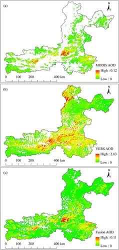
Because of the different overpass times of the Terra and Aqua satellites, there were some systematic biases between them; therefore, OLS regression was conducted to obtain the fused AOD when Terra and Aqua AOD data were present. Regression equations were then applied to predict the missing Aqua AOD using Terra AOD, which was present, and vice versa. For both products were missing, VIIRS AOD was used instead. The overpass time of the VIIRS was the same as that of Aqua. OLS regression was used to define the relationships between them, and the existing VIIRS AOD was used to predict the missing values. For example, there was a serious lack of MODIS AOD in January (only 38% data) due to the poor retrieval of bright surfaces and high levels of pollution in winter (Ma et al. 2016c), and the spatial coverage of VIIRS AOD data in the study area was 81% in January. Finally, the fusion of the three AOD datasets achieved 87% space coverage in January (Figure 2). The results showed that the combination of MODIS AOD and VIIRS AOD was useful for improving AOD coverage.

Figure 2. The spatial distribution of the aerosol optical depth (AOD) product from different satellites in January. (a) Moderate Resolution Imaging Spectroradiometer (MODIS) AOD, (b) Visible Infrared Imaging Radiometer Suite (VIIRS) AOD, and (c) AOD after the fusion of the MODIS and VIIRS data.

3.2. Descriptive statistics

The study area was divided into 3 × 3 km grids. AOD, PBLH, RH, TEM, PREP, WS, and NDVI were determined for each grid. If there were multiple data in the grid, the average value was used to ensure that each grid had unique AOD, PBLH, RH, TEM, PREP, WS, and NDVI values. The distribution of all factors was determined for each month (Supporting Information (SI), Figure S1). The AOD values were high from March to August, with a mean value of 0.08, but were low from January to February and in December, with a mean value of 0.01. The average AOD value was higher in the plains (0.16) than in the mountainous areas (0.03). The PBLH exhibited obvious spatio-temporal variations. The PBLH was high (510–567 m) from April to June and low (285–298 m) in January and from November to December. The average PBLH at a high latitude (485 m) was higher than that at a low latitude (351 m), indicating that the vertical diffusion condition at high latitudes was better. The RH was high (49–70%) in summer and low (32–58%) in winter and spring. In addition, there was obvious spatial heterogeneity of RH; the average values of RH in the mountainous region (59.4%) were higher than those in the valleys (48.3%). Temporal and spatial variations of TEM were consistent with PREP, with high temperature (average temperature of 25°C) and rainfall (total precipitation of 1,052 mm) in summer, and low temperature (average value of −3.4°C) and rainfall (total precipitation of 151 mm) in winter. The WS was low (0.96 m/s) throughout the study area, but was relatively high (1.52–1.77 m/s) in July and August. In the southern region, WS was low (average value of 0.66 m/s) in winter, which proved that the diffusion condition in the region was unfavorable. The average NDVI was high (0.7) in summer and low in winter (0.2). A lower NDVI indicated that there was less vegetation cover and large areas of bare land. In conclusion, the low PBLH and WS, high RH, and basin topography explain the poor diffusion conditions in the southern valleys, particularly in winter. In contrast, higher PBLH and WS values favored good diffusion conditions in the north of the study area.

3.3. Model fitting and the 10-fold CV

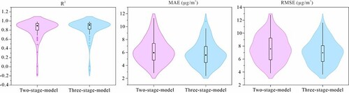
The two-stage model is constructed using the two stages of temporal and spatial models (Ma et al. 2016a; Zhang et al. 2021). In the present study, the two-stage model was constructed using stage-2 and stage-3, which were mainly used for comparison with the three-stage model. The R², MAE, and RMSE values of the different models were determined using environmental monitoring sites (Figure 3). The R² value of both models ranged from 0.80 to 0.95, excluding the discrete values, indicating that both models had a good simulation effect. Remarkably, the average MAE and RMSE values of the three-stage model were lower (0.4 and 0.6 μg/m³, respectively) than those of the two-stage model, respectively. The data distribution of the three-stage model was more concentrated. Therefore, the error between the predicted and observed concentrations was smaller in the three-stage model. In summary, the R², MAE, and RMSE values proved that the three-stage model performed better than the two-stage model, and demonstrated that stage-1 of the three-stage model could improve the accuracy of the model fit.

Figure 3. Violin plot with box plots of the estimation performance of the different models at each site, showing the R², mean absolute error (µg/m³), and root mean square error (µg/m³). (Black boxes represent quartiles, black dots represent median values, and colorful dots represent discrete values.)

The results of the 10-fold CV for both models are shown in Figure 4. The CV R² values of the three- and two-stage model were 0.92 and 0.90, respectively. They were lower (by 0.04 and 0.05) than the original R² values, respectively, indicating slight overfitting in both models. Based on the high model CV R², the AOD-PM_2.5 equation was established using the three-stage model in this study.

Figure 4. Scatterplots of the cross-validation results for the different models.

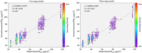
In stage-1, the range of the corrected AOD was from 0 to 0.00066, and the average corrected AOD was 0.000058 (Table 1). In stage-2, the fixed slope and intercept were 26544.51 and 57.14 (p < 0.0001), respectively. The average random residual was 0.07, and the standard deviations of the random slope and intercept were 35504.31 and 27.57, respectively. In stage-3, TEM and PREP had a collinearity problem; one or neither of them were integrated into the model, whereas other parameters could be entered into the GWR model each time. Finally, 647 pairs of PM_2.5-AOD matching points were used to create the model. The three-stage model fitting CV R² of the whole study area was 0.92, and the MAE and RMSE were 5.72 and 7.15 µg/m³, respectively. Overall, 92% of the observation values were interpreted using the predicted PM_2.5.

Table 1. The AOD and corrected AOD values.

Date	AOD			Revised AOD
	Min	Max	Mean	Min	Max	Mean
Jan.	0	0.11	0.0075	0	0.00014	0.000011
Feb.	0	0.23	0.0277	0	0.00042	0.000044
Mar.	0	0.61	0.0949	0	0.00039	0.000095
Apr.	0	0.42	0.1005	0	0.00046	0.000099
May.	0	0.33	0.0804	0	0.00066	0.000098
Jun.	0	0.29	0.0708	0	0.00028	0.000066
Jul.	0	0.40	0.0599	0	0.00029	0.000040
Aug.	0	0.52	0.0948	0	0.00042	0.000074
Sep.	0	0.20	0.0412	0	0.00022	0.000042
Oct.	0	0.45	0.0767	0	0.00064	0.000010
Nov.	0	0.27	0.0553	0	0.00048	0.000099
Dec.	0	0.09	0.0089	0	0.00024	0.000021
Yearly	0	0.33	0.0599	0	0.00039	0.000058

3.4. Predicted PM_2.5 concentrations

A three-stage model was established to estimate PM_2.5 concentrations. Those that were estimated by the model had a smaller error compared with the monitored data, and the estimated result had more detailed spatial distribution characteristics. Hence, it could provide basic data support for air pollution control and PM_2.5 health risk assessment. The results were expressed in three different timescales: year, season, and month (Figures 5 and 6). In 2018, the annual predicted PM_2.5 concentrations ranged from 57 to 64 µg/m³, with an average concentration of 58.76 µg/m³. The average annual observed PM_2.5 concentration was 58.66 µg/m³ in the same period. The estimated and observed PM_2.5 concentrations were approximately 58.71 (± 0.05) µg/m³. The advantage of the estimated PM_2.5 concentration was that it could show more abundant spatial information in areas without monitoring stations.

Figure 5. The annual, seasonal, and monthly PM_2.5 concentrations estimated based on the three-stage model in the Fenwei Plain.

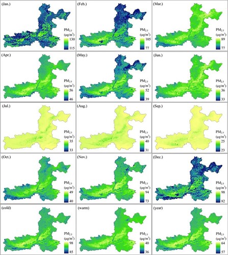
Figure 6. The differences between estimated and observed PM_2.5 concentrations in different time-scales.

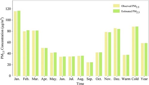
There were obvious seasonal differences in PM_2.5 concentrations in the Fenwei Plain (Figures 5 and 6). April to October (no-heating season) were taken as the warm season, and January to March and November to December (heating season) were taken as the cold season to analyze the seasonal change in PM_2.5 concentration. PM_2.5 concentrations in the warm season ranged from 36 to 40 µg/m³, with an average of 37.68 µg/m³. In the cold season, the range of PM_2.5 concentrations was 85–98 µg/m³, with an average of 88.28 µg/m³. The average PM_2.5 concentration in the cold season was more than 2.3 times as much as that in the warm season. Comparing estimated with observed concentrations in warm and cold seasons, the difference in the warm season (37.58 µg/m³) was 0.10 µg/m³, and the difference in the cold season (88.18 µg/m³) was also 0.10 µg/m³. The deviation between the estimated and measured PM_2.5 concentrations was small, which indicated that the accuracy of the seasonal estimation was high.

The differences in PM_2.5 concentrations between different months were relatively large (Figures 5 and 6). The PM_2.5 concentrations were high in January to March, November, and December (the average concentration was 116.54, 81.71, 81.16, 78.02, and 83.97 µg/m³, respectively). Relatively low concentrations (< 50 µg/m³) occurred during April–October. The overall deviation for all months was small (average difference of 0.5 µg/m³). Therefore, the monthly PM_2.5 concentrations could be estimated properly using the three-stage model.

To better analyze the spatial differences, the area with a Digital Elevation Model (DEM) > 500 m was defined as a mountainous area, the area with a DEM < 500 m was defined as a plains area, and the high pollution areas were mainly concentrated in the plains. The average deviation of estimated and observed PM_2.5 was −1.47 µg/m³ in the plains and 2.87 µg/m³ in the mountainous areas. The overall deviation was relatively small in the study area (average difference of 1.4 µg/m³). Therefore, the three-stage model performed well for PM_2.5 estimated concentrations.

4. Discussion

In this study, a three-stage model was developed to estimate PM_2.5 concentrations for the Fenwei Plain. Compared with the multi-stage machine learning model (Schneider et al. 2020), two-stage model (Zhang et al. 2021), geostatistical regression, and restricted geostatistical regression (Beloconi et al. 2018), the three-stage model had a better fitting effect (CV R² of 0.92) in this study. Based on the two-stage model, stage-1 was added based on physical processes to develop a three-stage model, and higher CV R² and lower MAE and RMSE were reported than those of the two-stage model. Although many studies have used PBLH and RH as auxiliary factors involved in model construction (Ma et al. 2014; Yang, Xu, and Jin 2018; Yao et al. 2018), the weights of PBLH and RH were the same as those of other auxiliary factors, and these two factors were not well-explained by these methods. In the present study, the weights of the vertical-and-RH correction models were increased based on physical interpretation, and the results of this study were more accurate. Therefore, it is necessary to correct AOD using stage-1.

The results of this study proved that the fusion of the VIIRS AOD and MODIS AOD can reduce AOD gaps. There are many satellite-sensor AOD products that can be used for data fusion, such as Multiangle Imaging Spectro Radiometer (MISR) 4.4 km AOD, Sea and Land Surface Temperature Radiometer (SLSTR) 10 km AOD, MODIS 10 km AOD, MODIS 3 km AOD, and VIIRS 6 km AOD. The MISR AOD has the smallest data bias, but it has the least amount of data (Choi et al. 2019). In contrast with the MODIS, on the one hand, the SLSTR AOD differs in terms of aerosol retrieval algorithm. On the other hand, the SLSTR AOD is limited in terms of spatial resolution (10 km) because of the smaller scan width (Handschuh et al. 2022). The data quality and quantity of the MODIS 10 km product is similar to that of the MODIS 3 km product, but its coarse spatial resolution does not meet the needs of urban studies, while MODIS 3 km can not only meet the data quality requirements but also obtain more data (Remer et al. 2013). The AOD inversion algorithm of VIIRS is similar to that of the MODIS algorithm, and the spatio-temporal coverage of the VIIRS AOD is very significant in winter (Yao et al. 2018), which compensates for the lack of MODIS AOD. Here, the VIIRS 6 km AOD and MODIS 3 km AOD were chosen to achieve the data fusion of AOD. The results proved that the fusion of VIIRS AOD and MODIS AOD was effective in the Fenwei Plain. Meanwhile, the OLS fusion method was more effective than the fusion method at averaging multiple data because it could eliminate systematic differences in satellite-observed AOD (Ma et al. 2014; Puttaswamy et al. 2014). In the present study, the model performed better after using the OLS method for AOD. The model CV R² of the OLS method improved by 0.02 compared to the average data. Other studies could use this method to fill AOD gaps and enhance the fitting effect of the model.

The present study had some limitations as well as some prospects. First, the deviations between the estimated and monitored concentrations were large (average difference of 1.19 µg/m³) in January, February, November, and December, which were seriously polluted. In future research, it will be essential to improve the fitted accuracy in the winter months. The estimated deviations for different terrain conditions were calculated based on sites (SI, Table S1), and the results showed that there was a problem of underestimation in the plains and overestimation in the mountains; therefore, the topographical conditions should be an area of focus in future studies. Second, 1 km AOD products (Multiangle Implementation of Atmospheric Correction [MAIAC] AOD) have been utilized to estimate PM_2.5 concentrations, and 1 km products have improved the spatial resolution and inversion algorithms (Li et al. 2020a; Jin et al. 2021). In future studies, the spatial resolution of ground-level PM_2.5 concentration estimation could be improved by MAIAC AOD.

5. Conclusions

This is one of the first studies, to our knowledge, to assess the performance of a fusion of MODIS AOD and VIIRS AOD for PM_2.5 concentrations estimated using a three-stage model. The results showed that when using the OLS method to fuse the MODIS 3 km AOD and VIIRS 6 km AOD, the fusion AOD could fill data gaps for winter. In addition, when a stage-1 base was added to vertical-and-RH correction of the AOD to develop a three-stage model, the estimation accuracy was higher than when using a two-stage model. The results indicated that CV R² of the three-stage model was 0.92, while the MAE and RMSE were 5.72 and 7.15 µg/m³, respectively. In brief, the three-stage model incorporating the MODIS and VIIRS AOD achieved high accuracy in regional ground-level PM_2.5 concentration estimation and provided a foundation for further regional PM_2.5 exposure and air pollution studies.

Acknowledgments

We thank NASA, NOAA and the China National Environmental Monitoring Centre for providing data.

Data availability statement

The data that support the findings of this study are openly available in the Open Science Framework data repository.

Disclosure statement

No potential conflict of interest was reported by the author(s).

Additional information

Funding

The research was supported by National Key Research and Development Program [grants number 2016YFC0201700].

References

- Beloconi, A., N. Chrysoulakis, A. Lyapustin, J. Utzinger, and P. Vounatsou. 2018. “Bayesian Geostatistical Modelling of PM10 and PM2.5 Surface Level Concentrations in Europe Using High-Resolution Satellite-Derived Products.” Environment International 121 (1): 57–70. doi:10.1016/j.envint.2018.08.041.
- Bian, J. H., A. N. Li, C. Q. Huang, R. Zhang, and X. W. Zhan. 2018. “A Self-Adaptive Approach for Producing Clear-Sky Composites from VIIRS Surface Reflectance Datasets.” ISPRS Journal of Photogrammetry and Remote Sensing 144: 189–201. doi:10.1016/j.isprsjprs.2018.07.009
- Chen, H., Q. Li, Z. T. Wang, H. Q. Mao, C. Y. Zhou, L. J. Zhang, and X. L. Chou. 2014. “Study on Monitoring Surface PM2.5 Concentration in Jing-Jin-Ji Regions Using MODIS Data.” Journal of Meteorology and Environment 30 (5): 27–37. doi:10.3969/j.issn.1673-503X.2014.05.005.
- Chen, H., Q. Li, Y. H. Zhang, C. Y. Zhou, and Z. T. Wang. 2016. “Estimations of PM2.5 Concentrations Based on the Method of Geographically Weighted Regression.” Acta Scientiae Circumstantiae 36 (6): 2142–2151. doi:10.13671/j.hjkxxb.2015.0780.
- Chen, W. Q., H. F. Ran, X. Y. Cao, J. Z. Wang, D. X. Teng, J. Chen, and X. Zheng. 2020. “Estimating PM2.5 with High-Resolution 1-km AOD Data and an Improved Machine Learning Model Over Shenzhen, China.” Science of the Total Environment 746: 141093. doi:10.1016/j.scitotenv.2020.141093.
- Chen, Z. Y., T. H. Zhang, R. Zhang, Z. M. Zhu, J. Yang, P. Y. Chen, C. Q. Ou, and Y. M. Guo. 2019. “Extreme Gradient Boosting Model to Estimate PM2.5 Concentrations with Missing-Filled Satellite Data in China.” Atmospheric Environment 202: 180–189. doi:10.1016/j.atmosenv.2019.01.027.
- Choi, M., H. Lim, J. Kim, S. Lee, T. F. Eck, B. N. Holben, M. J. Garay, E. J. Hyer, P. E. Saide, and H. Q. Liu. 2019. “Validation, Comparison, and Integration of GOCI, AHI, MODIS, MISR, and VIIRS Aerosol Optical Depth Over East Asia During the 2016 KORUS-AQ Campaign.” Atmospheric Measurement Techniques 12: 4619–4641. doi:10.5194/amt-12-4619-2019
- Cong, N., S. L. Piao, A. P. Chen, X. H. Wang, X. Lin, S. P. Chen, S. J. Han, G. S. Zhou, and X. P. Zhang. 2012. “Spring Vegetation Green-up Date in China Inferred from SPOT NDVI Data: A Multiple Model Analysis.” Agricultural and Forest Meteorology 165: 104–113. doi:10.1016/j.agrformet.2012.06.009.
- Donkelaar, A. V., R. V. Martin, R. J. D. Spurr, and R. T. Burnett. 2015. “High-resolution Satellite-Derived PM2.5 from Optimal Estimation and Geographically Weighted Regression Over North America.” Environmental Science & Technology 49 (17): 10482–10491. doi:10.1021/acs.est.5b02076.
- Engel-Cox, J. A., C. H. Holloman, B. W. Coutant, and R. M. Hoff. 2004. “Qualitative and Quantitative Evaluation of MODIS Satellite Sensor Data for Regional and Urban Scale air Quality.” Atmospheric Environment 38 (16): 2495–2509. doi:10.1016/j.atmosenv.2004.01.039.
- Fotheringham, A. S., C. F. Brunsdon, and M. E. Charlton. 2002. “Geographically Weighted Regression: The Analysis of Spatially Varying Relationships.”
- Guo, J. P., Y. R. Wu, X. Y. Zhang, and X. W. Li. 2013. “Estimation of PM2.5 Over Eastern China from MODIS Aerosol Optical Depth Using the Back Propagation Neural Network.” Environmental Science 34 (03): 817–825. doi:CNKI:SUN:HJKZ.0.2013-03-002.
- Gupta, P., S. A. Christopher, J. Wang, R. Gehrig, Y. Lee, and N. Kumar. 2006. “Satellite Remote Sensing of Particulate Matter and Air Quality Assessment Over Global Cities.” Atmospheric Environment 40 (30): 5880–5892. doi:10.1016/j.atmosenv.2006.03.016.
- Handschuh, J., T. Erbertseder, M. Schaap, and F. Baier. 2022. “Estimating PM2.5 Surface Concentrations from AOD: A Combination of SLSTR and MODIS.” Remote Sensing Applications: Society and Environment 26: 100716. doi:10.1016/j.rsase.2022.100716.
- He, Q. Q., and B. Huang. 2018a. “Satellite-based High-Resolution PM2.5 Estimation Over the Beijing-Tianjin-Hebei Region of China Using an Improved Geographically and Temporally Weighted Regression Model.” Environmental Pollution 236: 1027–1037. doi:10.1016/j.envpol.2018.01.053.
- He, Q. Q., and B. Huang. 2018b. “Satellite-based Mapping of Daily High-Resolution Ground PM2.5 in China via Space-Time Regression Modeling.” Remote Sensing of Environment 206: 72–83. doi:10.1016/j.rse.2017.12.018.
- Hoogh, K. D., H. Héritier, M. Stafoggia, N. Künzli, and I. Kloog. 2018. “Modelling Daily PM2.5 Concentrations at High Spatio-Temporal Resolution Across Switzerland.” Environmental Pollution 233: 1147–1154. doi:10.1016/j.envpol.2017.10.025.
- Hu, X. F., L. A. Waller, A. Lyapustin, Y. J. Wang, M. Z. Al-Hamdan, W. L. Crosson, M. G. Estes Jr., et al. 2014. “Estimating Ground-Level PM2.5 Concentrations in the Southeastern United States Using MAIAC AOD Retrievals and a Two-Stage Mode.” Remote Sensing of Environment 140: 220–232. doi:10.1016/j.rse.2013.08.032.
- Jackson, J. M., H. Q. Liu, L. Laszlo, S. Kondragunta, L. A. Remer, J. F. Huang, and H. C. Huang. 2013. “Suomi-NPP VIIRS Aerosol Algorithms and Data Products.” Journal of Geophysical Research: Atmospheres 118: 12,673–12,689. doi:10.1002/2013JD020449.
- Jin, J. N., X. C. Yang, X. Yan, and W. J. Zhao. 2021. “MAIAC AOD and PM2.5 Mass Concentrations Characteristics and Correlation Analysis in Beijing-Tian-Hebei and Surrounding Areas.” Environmental Science 42 (6): 2604–2615. doi:10.13227/j.hjkx.202009200.
- Jing, Y., Y. L. Sun, H. Xu, L. Chen, H. Zhang, S. Gao, H. C. Fu, and J. Mao. 2018. “Daily Estimation of PM2.5 Concentrations Based on Mixed Effects Model in Beijing-Tianjin-Heibei Region.” China Environmental Science 8: 2890–2897. doi:CNKI:SUN:ZGHJ.0.2018-08-013.
- Karimian, H., Q. Li, C. C. Li, J. Fan, L. Jin, C. Gong, Y. Mo, J. Hou, and A. Ahmad. 2017. “Daily Estimation of Fine Particulate Matter Mass Concentration Through Satellite Based Aerosol Optical Depth.” ISPRS Annals of Photogrammetry, Remote Sensing and Spatial Information Sciences IV-4/W2: 175–181. doi:10.5194/isprs-annals-IV-4-W2-175-2017.
- Lee, H. J., Y. Liu, B. A. Coull, J. Schwartz, and P. Koutrakis. 2011. “A Novel Calibration Approach of MODIS AOD Data to Predict PM2.5 Concentrations.” Atmospheric Chemistry & Physics 11: 7991–8002. doi:10.5194/acp-11-7991-2011.
- Li, L. F., M. Franklin, M. Girguis, F. Lurmann, J. Wu, N. Pavlovic, C. Breton, F. Gilliland, and R. Habre. 2020a. “Spatiotemporal Imputation of MAIAC AOD Using Deep Learning with Downscaling.” Remote Sensing of Environment 237: 111584. doi:10.1016/j.rse.2019.111584.
- Li, Y., G. P. Shi, and Z. A. Sun. 2020b. “Evaluation and Improvement of MODIS Aerosol Optical Depth Products Over China.” Atmospheric Environment 223: 117251. doi:10.1016/j.atmosenv.2019.117251.
- Liu, H., X. M. Gao, Z. Y. Xie, T. T. Li, and W. J. Zhang. 2015. “Spatio-temporal Characteristics of Aerosol Optical Depth Over Beijing-Tianjin-Hebei-Shanxi-Shandong Region During 2000-2013.” Acta Scientiae Circumstantiae 35 (5): 1506–1511. doi:10.13671/j.hjkxxb.2014.0949.
- Liu, H. Q., L. A. Remer, J. F. Huang, H. C. Huang, S. Kondragunta, I. Laszlo, M. Oo, and J. M. Jackson. 2014. “Preliminary Evaluation of S-NPP VIIRS Aerosol Optical Thickness.” Journal of Geophysical Research Atmospheres 119: 3942–3962. doi:10.1002/2013JD020360.
- Lv, B. L., Y. T. Hu, H. H. Chang, A. G. Russell, and Y. Q. Bai. 2016. “Improving the Accuracy of Daily PM2.5 Distributions Derived from the Fusion of Ground-Level Measurements with Aerosol Optical Depth Observations, a Case Study in North China.” Environmental Science & Technology 50 (9): 4752–4759. doi:10.1021/acs.est.5b05940.
- Lv, B. L., Y. T. Hu, H. H. Chang, A. G. Russell, J. Cai, B. Xu, and Y. Q. Bai. 2017. “Daily Estimation of Ground-Level PM2.5 Concentrations at 4 km Resolution Over Beijing-Tianjin-Hebei by Fusing MODIS AOD and Ground Observations.” Science of the Total Environment 580: 235–244. doi:10.1016/j.scitotenv.2016.12.049.
- Ma, Z. W., X. F. Hu, L. Huang, J. Bi, and Y. Liu. 2014. “Estimating Ground-Level PM2.5 in China Using Satellite Remote Sensing.” Environmental Science & Technology 48 (13): 7436–7444. doi:10.1021/es5009399.
- Ma, Z. W., X. F. Hu, A. M. Sayer, R. Levy, Q. Zhang, Y. A. Xue, S. L. Tong, J. Bi, L. Huang, and Y. Liu. 2016a. “Satellite-Based Spatiotemporal Trends in PM2.5 Concentrations: China, 2004–2013.” Environmental Health Perspectives 124 (2): 184–192. doi:10.1289/ehp.1409481.
- Ma, Z. W., Y. Liu, Q. Y. Zhao, M. M. Liu, Y. C. Zhou, and J. Bi. 2016b. “Satellite-derived High Resolution PM2.5 Concentrations in Yangtze River Delta Region of China Using Improved Linear Mixed Effects Model.” Atmospheric Environment 133: 156–164. doi:10.1016/j.atmosenv.2016.03.040.
- Ma, X. Y., J. Y. Wang, F. Q. Yu, H. L. Jia, and Y. A. Hu. 2016c. “Can MODIS AOD be Employed to Derive PM2.5 in Beijing-Tianjin-Hebei Over China?” Atmospheric Research 181: 250–256. doi:10.1016/j.atmosres.2016.06.018.
- Munchak, L. A., R. C. Levy, S. Mattoo, L. A. Remer, B. N. Holben, J. S. Schafer, C. A. Hostetler, and R. A. Ferrare. 2013. “MODIS 3 km Aerosol Product: Applications Over Land in an Urban/Suburban Region.” Atmospheric Measurement Techniques 6 (7): 1747–1759. doi:10.5194/amt-6-1747-2013.
- Natunen, A., A. Arola, T. Mielonen, J. Huttunen, M. Komppula, and K. E. J. Lehtinen. 2010. “A Multi-Year Comparison of PM2.5 and AOD for the Helsinki Region.” Boreal Environment Research 15 (6): 544–552. doi:10.1029/2010WR009092.
- Puttaswamy, S. J., H. M. Nguyen, A. Braverman, X. F. Hu, and Y. Liu. 2014. “Statistical Data Fusion of Multi-Sensor AOD Over the Continental United States.” Geocarto International 29 (1): 48–64. doi:10.1080/10106049.2013.827750.
- Remer, L. A., S. Mattoo, R. C. Levy, and L. A. Munchak. 2013. “MODIS 3 km Aerosol Product: Algorithm and Global Perspective.” Atmospheric Measurement Techniques 6: 1829–1844. doi:10.5194/amt-6-1829-2013.
- Schneider, R., A. M. Vicedo-Cabrera, F. Sera, P. Masselot, M. Stafoggia, K. D. Hoogh, I. Kloog, S. Reis, M. Vieno, and A. Gasparrini. 2020. “A Satellite-Based Spatio-Temporal Machine Learning Model to Reconstruct Daily PM2.5 Concentrations Across Great Britain.” Remote Sensing 12 (22): 3803. doi:10.3390/rs12223803.
- Sun, J. Y., N. Zhang, X. N. Yan, M. Wang, and J. Wang. 2020. “The Effect of Ambient Fine Particulate Matter (PM2.5) on Respiratory Diseases in China: A Systematic Review and Meta-Analysis.” Stochastic Environmental Research and Risk Assessment 34: 593–610. doi:10.1007/s00477-020-01786-0.
- Tan, W. Z. 2007. The Basic Theoretics and Application Research on Geographically Weighted Regression. Shanghai, China: Tongji University.
- Wang, Z. F., L. F. Chen, J. H. Tao, Y. Zhang, and L. Su. 2010. “Satellite-based Estimation of Regional Particulate Matter (PM) in Beijing Using Vertical-and-RH Correcting Method.” Remote Sensing of Environment 114 (1): 50–63. doi:10.1016/j.rse.2009.08.009.
- Wang, C. L., Y. Y. Wang, Z. H. Shi, J. J. Sun, K. J. Gong, J. Y. Li, M. M. Qin, J. Wei, H. D. Kan, and J. L. Hu. 2021. “Effects of Using Different Exposure Data to Estimate Changes in Premature Mortality Attributable to PM2.5 and O3 in China.” Environmental Pollution 285: 117242. doi:10.1016/j.envpol.2021.117242.
- White, W. H., and P. T. Roberts. 1977. “On the Nature and Origins of Visibility-Reducing Aerosols in the Los Angeles air Basin.” Atmospheric Environment 11 (9): 803–812. doi:10.1016/0004-6981(77)90042-7.
- Wu, J. S., W. D. Xie, and J. C. Li. 2016. “Application of Land-use Regression Models in Spatial-Temporal Differentiation of Air Pollution.” Environmental Science 37 (02): 413–419. doi:10.13227/j.hjkx.2016.02.002.
- Xie, Y. Y., Y. X. Wang, K. Zhang, W. H. Dong, B. L. Lv, and Y. Q. Bai. 2015. “Daily Estimation of Ground-Level PM2.5 Concentrations Over Beijing Using 3 km Resolution MODIS AOD.” Environmental Science & Technology 49 (20): 12280–12288. doi:10.1021/acs.est.5b01413.
- Xu, G., L. M. Jiao, F. T. Xiao, S. L. Zhao, and X. Zhang. 2016. “Applying Land use Regression Model to Estimate Spatial Distribution of PM2.5 Concentration in Beijing-Tianjin-Hebei Region.” Journal of Arid Land Resources and Environment 30 (10): 116–120. doi:CNKI:SUN:GHZH.0.2016-10-020.
- Yang, L. J., H. Q. Xu, and Z. F. Jin. 2018. “Estimating Spatial Variability of Ground-Level PM2.5 Based on a Satellite-Derived Aerosol Optical Depth Product: Fuzhou, China.” Atmospheric Pollution Research 9 (6): 1194–1203. doi:10.1016/j.apr.2018.05.007.
- Yang, Z. M., C. Zdanski, D. Farkas, J. Bang, and H. Williams. 2020. “Evaluation of Aerosol Optical Depth (AOD) and PM2.5 Associations for air Quality Assessment.” Remote Sensing Applications Society and Environment 20: 100396. doi:10.1016/j.rsase.2020.100396.
- Yao, F., M. L. Si, W. F. Li, and J. S. Wu. 2018. “A Multidimensional Comparison Between MODIS and VIIRS AOD in Estimating Ground-Level PM2.5 Concentrations Over a Heavily Polluted Region in China.” Science of the Total Environment 618: 819–828. doi:10.1016/j.scitotenv.2017.08.209.
- Zhang, Y., Z. Q. Li, Y. Y. Wei, and Z. R. Peng. 2021. “A Satellite-Derived, Ground-Measurement-Independent Monthly PM2.5 Mass Concentration Dataset Over China During 2000–2015.” Big Earth Data 1918908. doi:10.1080/20964471.2021.1918908.