Mapping groundwater dependent ecosystem potential in a semi-arid environment using a remote sensing-based multiple-lines-of-evidence approach

ABSTRACT

Groundwater dependent ecosystems (GDEs) are vulnerable to groundwater regime changes. However, their protection is often hampered by challenges in their identification. Within is presented a remote sensing-based GDE potential mapping approach based on the persistency of relevant vegetation parameters during prolonged dry periods as an indicator of potential ‘consistency’ of water supply (e.g. groundwater). The study uses a novel approach to characterising persistency for selected vegetation parameters based on a normalised difference measure and an adaptation of the coefficient of variation statistic. Aggregation of parameters was facilitated through the analytic hierarchy process providing a structured weighting approach to minimise parameter bias. The approach is demonstrated in the semi-arid Flinders Ranges of South Australia where new groundwater resources are being sought to support local domestic and industry needs. Variations in GDE potential were mapped to better target areas where exploration of groundwater should be avoided. Mapping results indicated a high-level of agreement of 77% with an independent springs dataset, along with an 87% agreement with areas coinciding with known phreatophyte species and depths to groundwater. The index-based mapping approach has potential applicability across landscapes, as it normalises for variations in vegetation cover, minimises technical overheads, and employs continental-wide remote sensing data-products.

KEYWORDS:

• coefficient of variation NDVI
• coefficient of variation fractional cover
• barest Earth
• wetness percentiles
• actual evapotranspiration
• analytic hierarchy process
• groundwater potential

1. Introduction

Groundwater plays a critical role in providing water for the environment, industry, agriculture and to billions of people across the globe. But as world population increases and climate changes, sustainable supplies are becoming depleted, with recent reports acknowledging the oversubscription of groundwater resources at both regional and global scales (Garg et al. 2022; Bierkens and Wada 2019; Döll et al. 2014).

Of environmental significance, local and regional groundwater depletion threatens groundwater dependent ecosystems (GDEs) by reducing baseflow to rivers, lakes, wetlands, and groundwater levels beyond the root zone of phreatophytic vegetation. GDEs are ‘natural ecosystems that require access to groundwater to meet all or some of their water requirements on a permanent or intermittent basis so as to maintain their communities of plants and animals, ecological processes and ecosystem services’ (Richardson et al. 2011, 92). GDEs may include ecosystems dependent on the surface expression of groundwater, such as rivers, wetlands, springs, and lakes (aquatic ecosystems), the interaction of water below the ground level, including water in the capillary zone (terrestrial ecosystems) and the subterranean presence of groundwater (i.e. cave ecosystems), where the latter is not relevant to this study.

GDEs are vulnerable to groundwater regime changes that exceed the natural bounds of variation, threatening the important ecosystem services they provide, such as biodiversity, flood and erosion control, filtration, fish production, forestry and agriculture, and social values such as recreation and tourism (Doody et al. 2017). This is often caused by prolonged droughts and/or from over-abstraction for irrigation, drinking water or other developments which rely on groundwater for process and production (e.g. mining; Doody, Hancock, and Pritchard 2019). Their vulnerability may be exacerbated in semi-arid to arid climatic zones where water resources are scarce, and groundwater recharge is low, irregular, and localised, and where there are competing interests between human and environmental water needs.

While the protection of GDEs is an important component of sustainable water resource management, their protection is often hampered by challenges in their identification, the first requisite step towards their management (Eamus et al. 2015). GDE functioning is controlled by complex factors across temporal and spatial scales (Doody et al. 2009). Work by Doody (2019, 2017) and Eamus (2016, 2015) provide useful overviews of various methods used to help identify GDEs in these contexts. While in-situ field measurements, such as pre-dawn leaf water potentials and isotope analysis, may provide reliable identification of groundwater use by plants, these localised deterministic measures are costly and impractical to be applied across broader regional landscapes.

Alternatively, remote sensing methods have been used to provide a synoptic physiological landscape evaluation of the potential presence of GDEs. Differences between phreatophytic and xeric vegetation may be inferred by characterising their seasonal ‘spectral’ response where xeric vegetation may exhibit greater variation between wet and dry periods compared with phreatophytic vegetation (Barron et al. 2014). These differences have been exploited in multi-temporal remote sensing-based GDE studies using parameters such as greenness (Phiri, Shiferaw, and Tesfamichael 2018; Gou, Gonzales, and Miller 2015; Barron et al. 2014; Contreras et al. 2011; Tweed et al. 2007), wetness (Barron et al. 2014; Münch and Conrad 2007), structure (Castellazzi, Doody, and Peeters 2019), fractional cover (CDM Smith 2020), land surface temperature (Gow et al. 2016) and evapotranspiration (van Dijk et al. 2015). Methods of determining parameter persistency used as an indicator of potential consistency of water supply for plants, may include image classification (Xu et al. 2022; Barron et al. 2014), singular value decomposition (Brim Box et al. 2022), modelled relationship between vegetation greenness and groundwater depth (Duran-Llacer et al. 2022; Phiri, Shiferaw, and Tesfamichael 2018; Lv et al. 2013; Jin et al. 2011), high levels of evapotranspiration (van Dijk et al. 2015; Eamus et al. 2015) and most commonly where multi-temporal data sets are used, the incorporation of a variance measure such as standard deviation, to evaluate inter-annual or seasonal landscape dynamics (Xu et al. 2022; Castellazzi, Doody, and Peeters 2019; Gou, Gonzales, and Miller 2015; Lv et al. 2013; Dresel et al. 2010; Tweed et al. 2007).

Several parameters and/or methods using indicator spatial datasets may be combined such as land use/land cover, lithology, soil and vegetation type, depth to groundwater, flow accumulation, slope, drainage density, elevation, etc., tailored for specific eco-hydrological zones, for a more comprehensive multiple-lines-of-evidence or rule-set-based GDE identification approach. Thus, the mapping does not rely on the limitations of a single parameter alone, although many only serve to identify higher GDEP zones within which remote sensing methods are used to help identify the physiological hallmarks of groundwater dependence (Gou, Gonzales, and Miller 2015). This mapping approach has been applied at local scales (CDM Smith 2020; Rio Tinto 2020), regionally (Kuginis et al. 2016; QG 2015; White et al. 2014) and more comprehensively for the development of the national GDE Atlas of Australia (Doody et al. 2017; SKM and CSIRO 2012). However, developing these methods often requires a high degree of expert-knowledge, including the remote sensing methods and derived products that often underpin or moderate these rule-sets. Moreover, the rule-set-based approach typically reflects a classic multi-criteria decision analysis problem (Steele et al. 2009) where geographical information system (GIS)-based methods are used to combine preferentially weighted rules/parameters as judged by experts to map areas more likely to be GDEs. Notably, the ‘multi-criteria decision analysis’ approach is vulnerable to the behavioural biases affecting expert judgements in the decision-making process, which are usually conveyed into the weight assignment (Ferretti and Montibeller 2016). Among a range of factors, the assignment of parameter weights is considered the largest contributor to uncertainty in multi-criteria data analysis outputs (de Brito, Almoradie, and Evers 2019; Şalap-Ayça and Jankowski 2016; Chen, Yu, and Khan 2013). Yet very little justification is given to the parameter weighting method chosen in rule-set-based GDE mapping studies where the influence of one or more parameters may be over or under emphasised, resulting in potential variations in model outputs.

The aim of this study was to develop an effective multiple-lines-of-evidence GDE potential (GDEP) mapping approach using open-access datasets to perform multi-temporal evaluations of the persistency of relevant vegetation parameters during prolonged dry periods, including two greenness parameters, wetness, fractional cover, and evapotranspiration, as an indicator of possible ‘consistency’ of water supply. With increasing maturity of continental Earth observation data cubes, this study focuses on combining more ‘direct evidence’ physiological parameters, rather than including or placing more weight on ‘indirect’ zonal/topographic indicators to identify GDEs.

A novel characterisation of parameter persistency is demonstrated for greenness (NDVI), fractional cover and evapotranspiration, based on a normalised difference measure and a modified coefficient of variation statistic for the first two parameters. The GDEP mapping approach avoids the often-necessary expert-driven technical overheads or classification method nuances by combining ‘simple’ dimensionless parameter indices to yield a final GDEP ‘index’ more applicable across landscapes highlighting areas more likely to be GDEs. Parameters were combined using a weighted linear aggregation method for multiple criteria (parameters) where weights for each parameter were determined using an ‘objective’/structured approach to minimise parameter bias. While other weighting approaches can be used, we demonstrate the use of the analytic hierarchy process (AHP) first developed by Saaty (1977) to minimise the challenges of preferential weighting of multiple parameters/criteria simultaneously, frequently used in groundwater potential modelling research (Díaz-Alcaide and Martínez-Santos 2019).

The GDEP mapping approach is demonstrated surrounding the semi-arid/arid township of Leigh Creek in the northern Flinders Ranges of South Australia (Figure 1) where new groundwater resources are being sought to support domestic and industry needs (Somaratne 2019). The Flinders Ranges are almost completely dependent on natural springs and wells fed by groundwater stored in fractured rocks, to support the pastoral industry, mining, tourism and domestic use (Alcoe and Berens 2011; Clark and Brake 2008). Notably, dependence on groundwater for human consumption in the southern Flinders Ranges has increased resulting in a decline in water quality (Alcoe and Berens 2011). For the Leigh Creek region, little is known about the degree to which terrestrial vegetation is dependent upon groundwater, and thus their vulnerability to potential groundwater drawdown where new bores may be sited. The objective of this research was to identify the localised spatial variation in GDEP surrounding the township to better identify areas where exploration of groundwater should be avoided.

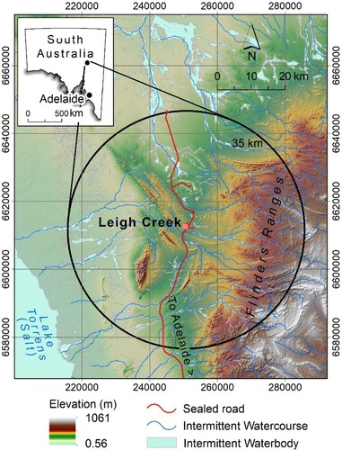
Figure 1. Study area defined by a 35 km radial zone (black line) around the township of Leigh Creek in the northern Flinders Ranges of South Australia (Longitude & Latitude: 138° 34′ 00″ E & 30° 35′ 36″ S). Map coordinate system showing Eastings and Northings, GDA94 UTM Map Grid of Australia (MGA) zone 54.

2. Methods

2.1. The Leigh Creek environs

The township of Leigh Creek is located approximately 500 km north of Adelaide (Figure 1). This semi-arid to arid region, experiences hot, dry Australian summers (mean January temperature, 35.8°C), cool to cold Australian winters (mean July temperature, 16.9°C), and has a low annual average rainfall of approximately 200 mm (BoM 2021). While groundwater exploration efforts undertaken by the South Australian Water Corporation (SA Water) will be restricted to areas within 10 km of the township, a larger 35 km radius was considered in this study to demonstrate the effectiveness of the GDEP mapping approach over a broader regional landscape.

The study area sits within a fractured rock geological setting, with hills and ridges in the east and central region of resistant Cambrian and Neoproterozoic quartzites, limestones and calcareous meta-siltstones. Centrally and to the west, these rocks are overlain by scree and alluvial deposits forming expansive plains to the west towards Lake Torrens. Except for minor supplies in recent alluvial deposits, most groundwater is sourced from fractured Neoproterozoic–Cambrian metasediments (Fildes et al. 2020). The valleys and plains are broken by stream channels (creeks) largely occupied by Eucalyptus trees (E. camaldulensis) (river red gum) with pockets of Melaleuca trees (M. glomerata) (inland paperbark). Vegetation in alluvial floodouts and run-on landforms adjacent creeks consist largely of Acacia victoriae (elegant wattle) over sparse chenopod species. Hills and ridges are dominated by sparse open woodlands of either Acacia aptaneura (mulga), Callitris glaucophylla (cypress-pine) or Casuarina pauper (belah), with some Triodia (tussock grass) or Cymbopogon (lemon grass) grassland areas (DEW 2022).

2.2. Method overview

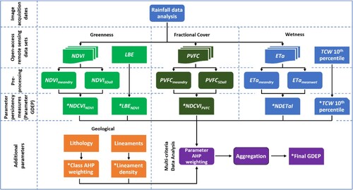
The proposed GDEP mapping method compares mean wet and mean prolonged dry period response of vegetation greenness, fractional cover, wetness, and actual evapotranspiration $(E{T}_a)$ (Figure 2). The assumption was made that a higher degree of persistency during prolonged dry periods for each parameter are indicators of possible groundwater interactions with vegetation (Castellazzi, Doody, and Peeters 2019; Doody, Hancock, and Pritchard 2019; Eamus et al. 2016; Gou, Gonzales, and Miller 2015; Barron et al. 2014; Dresel et al. 2010). Thus, an inverse relationship indicates soil moisture depletion and limited (or no) groundwater interaction with vegetation.

Figure 2. Overview of the GDEP model process. Persistency of greenness was measured using a ‘Normalised Difference Coefficient of Variation Index’ (NDCVI) derived from multiple surface reflectance and terrain corrected Landsat wet versus dry period NDVI images (NDCVI_NDVI). Persistency of photosynthetic vegetation fractional cover (PVFC) was also measured using a NDCVI (NDCVI_PVFC) derived from the same Landsat wet versus dry time-series, along with the persistency of vegetation and soil wetness measured using a ‘Normalised Difference Evapotranspiration Actual Index’ (ND$E{T}_a$I). Persistency of vegetation greenness and wetness was further measured using Landsat Barest Earth (LBE) NDVI (LBE_NDVI) and Tasselled Cap Wetness (TCW) 10th percentiles, respectively, independent of the Landsat image acquisition dates chosen for other parameters providing higher temporal and longer-term sampling. *Parameter outputs standardised to values between 0 and 1. Table S2 provides a summary description of each parameter and derived GDEP persistency model.

2.3. Landsat acquisition dates

A multi-date approach was used to compare mean inter-annual wet versus late dry period parameter statistics to avoid the localised spatio-temporal variability of rainfall and landscape response inherent when comparing only two, wet versus dry, image capture dates. A total of 26 cloud-free Landsat surface reflectance images (13 wet and 13 dry) were acquired for the period between 1987 and 2019 (Table S1). Dry period dates were chosen at the end of a distinct, prolonged dry period following a high rainfall event or prolonged wet period (BoM 2021); referred hereinafter as the ‘late dry period’ image date. A two-month approximate lag-time after peak green-up, evident in Landsat imagery using GloVis (2005), was chosen for the wet period dates to maximise perennial response while minimising the influence of green herbaceous/grass background where possible. Notably, the time between date pairs largely conformed with a study by Doody et al. (2015) that identified a substantial decrease in leaf area index as drying occurred for E. camaldulensis trees (which dominate the creek lines in this study area) approximately seven months after a substantial flood event in the Murray-Darling Basin in south-eastern Australia.

2.4. Persistency of vegetation greenness

The first approach used to evaluate the relative persistency of vegetation greenness employed the Normalised Difference Vegetation Index (NDVI) derived for each of the 26 Landsat images (Table S1) and an adaptation of the coefficient of variation (CV) statistic. The NDVI detects photosynthetically active biomass and is a reliable indicator of vegetation density, vigour and changes in vegetation patterns (Huang et al. 2020a). The CV is a measure of the relative dispersion of values around their mean, measured as a ratio of the standard deviation to the mean (SD/Mean). The higher the CV, the greater the dispersion, in this case, the difference between wet and late dry periods. The CV has been widely used for assessing inter-annual and seasonal variation in landscape greenness (e.g. Huang et al. 2020b; Yang et al. 2019; Schucknecht et al. 2017; Milich and Weiss 2000), and crop growth rate comparisons (e.g. Alharbi et al. 2019; Chanda et al. 2018). The advantage of using the CV over SD alone, is its ability to capture variations even when the mean [NDVI] value is very small (Mohan et al. 2018). This is typical of landscapes consisting of non-green vegetation (e.g. chenopods) or where green vegetation cover is low (Graetz, Pech, and Davis 1988).

In this study, the CV was adapted to use the SD calculated from all wet and late dry period NDVI images, per grid cell, to account for all inter-seasonal variation relative to the mean of all late dry period NDVI images only (locations that continue to exhibit photosynthetically active green vegetation during the late dry period). Thus, locations with a high late dry period NDVI mean (high late dry period greenness), with a low SD (minimal variation in greenness between wet and late dry periods), may indicate consistency of water supply with CV values closer to 0. It follows that the inverse of this relationship may indicate minimal or no groundwater interaction with vegetation (higher CV values). In this latter case, regeneration of actively growing green vegetation is likely affiliated with seasonal rainfall events where vegetation greenness is significantly higher during wet periods compared with dry periods. Intermediate CV values may indicate some connection with groundwater supply and thus the CV statistic can be used as a ‘persistency index’ of greenness.

A further adaptation of the CV was employed to linearise the ‘index’ and to standardise results with other mapped vegetation parameters (Malczewski 2000). This was achieved by taking the difference between the SD calculated from the combined wet and late dry period NDVI images $(NDV{I}_{SDall})$and the mean of the late dry period NDVI images $(NDV{I}_{Meandry})$, divided by their sum; referred to here as the ‘Normalised Difference Coefficient of Variation Index’ (NDCVI), that is: (1) $NDCV{I}_{NDVI}={\displaystyle \frac{NDV{I}_{Meandry}-NDV{I}_{SDall}}{NDV{I}_{Meandry}+NDV{I}_{SDall}},}$(1) where the NDVI subscript denotes the input data product to which the NDCVI output relates. The index has theoretical minimum and maximum values of −1 and +1, where the actual output range was subsequently rescaled to positive values between 0 and 1 for standardisation with other GDE indicator outputs, using: (2) ${\chi }^{\mathrm{\prime }}={\displaystyle \frac{\chi -{\chi }_{min}}{{\chi }_{max}-{\chi }_{min}},}$(2) where ${\chi }^{\mathrm{\prime }}$ is the new standardised (scaled) index value, $\chi$ is the value to be scaled (in this case the NDCVI value), and where ${\chi }_{min}$ and ${\chi }_{max}$ are the theoretical minimum and maximum values, respectively. Note that the NDCVI calculation is only suited to positive input values, thus only mean positive NDVI values > 0.15 were input to the procedure. This threshold value considered the higher NIR reflectance, relative to red, of bare soils over the study area, resulting in NDVI values > 0 and where White et al. (2016) identified similar dryland vegetation NDVI thresholds of 0.11–0.32 and 0.14–0.15 in South Australia. This site-specific threshold was determined through careful evaluation of high-resolution (< 40 cm) visible-NIR dry season aerial photography (DEWNR 2017) to delineate green vegetated areas (to include very low vegetated cover) from non-green areas (water, soil and plant litter background), and where the latter areas were masked as non-GDE locations.

The second approach used to evaluate the relative persistency of vegetation greenness took advantage of the recently developed Landsat ‘Barest Earth’ (LBE) product (Roberts, Wilford, and Ghattas 2019). The LBE mosaic of Australia (Wilford and Roberts 2019) was developed using a novel high-dimensional statistical technique to reveal the continent at its ‘barest state’ using 30+ years of Landsat data for unobstructed diagnostic mineral mapping. Notably, ‘remaining green areas in the Barest Earth mosaic indicate areas of persistent vegetation’ (Roberts, Wilford, and Ghattas 2019, 2) and may indicate consistency of water supply in climatic regions with distinct, prolonged dry periods. As the LBE product maintains spectral integrity between wavelengths, the red and NIR bands were used to generate an NDVI image of the study area (LBE_NDVI). A threshold of > 0.15 was again used to delineate vegetated from non-vegetated areas, where the full range of LBE_NDVI values (> 0.15) were rescaled between 0 and 1 using equation (2), complementing the NDCVI_NDVI results with a much higher-temporal and longer-term analysis.

2.5. Persistency of vegetation fractional cover

Fractional cover estimates the proportional/areal coverage of photosynthetic vegetation (green vegetation), non-photosynthetic vegetation (dry plant litter/material) and soil background per grid cell location where each [sub-pixel] component sums to 100%. An assumption was made that where photosynthetic vegetation (PV) coverage undergoes less change between wet and prolonged dry periods and areal coverage persists, it may indicate a consistent water supply, and vice versa.

This study employed the national Landsat 30 m Fractional Cover (FC) product developed by the Joint Remote Sensing Research Program (JRSRP) (DEA 2021). The JRSRP FC algorithm uses image derived endmembers for each fractional component, developed using multiple regression of field data, in a constrained (sum to 100%) spectral unmixing approach (Scarth, Röder, and Schmidt 2010). Mean and SD statistics were calculated for the PV component of the FC product derived from all 26 Landsat images (Table S1). The persistency of the PV component was then estimated using the NDCVI, such that: (3) $NDCV{I}_{PVFC}={\displaystyle \frac{PVF{C}_{Meandry}-PVF{C}_{SDall}}{PVF{C}_{Meandry}+PVF{C}_{SDall}},}$(3) where the PVFC subscript denotes the input data product to which the NDCVI output relates, $PVF{C}_{SDall}$ is the SD calculated from all wet and late dry period PVFC images, and $PVF{C}_{Meandry}$ is the mean of the late dry period PVFC images. Output index values (−1 to +1) were rescaled to values between 0 and 1 using equation (2).

2.6. Persistency of vegetation wetness

The first approach used to evaluate the relative persistency of vegetation wetness (including soil wetness in areas of low vegetation cover) employed Tasselled Cap Wetness (TCW) percentile summaries calculated from individual TCW images captured between 1987 and 2018 (DEA 2018). Individual TCW images were generated from reflectance factor coefficients developed by Crist (1985) to allow comparison between 30+ years of Landsat derived TCW images. For this semi-arid environment, high TCW 10th percentile values closer to 0 (with a negative index range between −7,000 and −120) represented fully saturated areas, such as water bodies, along with vegetated areas that have remained ‘wetter’ throughout dry periods with lower inter-seasonal differences and may indicate consistency of water supply. The TCW 10th percentile image was masked using a combined mean dry NDVI (from 13 dry period images, Table S1) and LBE_NDVI threshold value of > 0.15 to delineate the relative wetness of perennial vegetated areas only. The min–max range of the masked results were rescaled and standardised to values between 0 and 1 using equation (2).

The second approach used to evaluate relative persistency of vegetation wetness employed the recently released nation-wide actual evapotranspiration $(E{T}_a)$ dataset for Australia derived using the CSIRO¹ MODIS² reflectance-based scaling evapotranspiration (CMRSET) algorithm (Guerschman et al. 2022; McVicar et al. 2022). The current algorithm builds on the work by Guerschman et al. (2009), which, among other improvements, calibrates the CMRSET algorithm with higher resolution sensors such as VIIRS,³ Landsat and Sentinel-2, published as daily average $E{T}_a$ for each month at 30 m resolution (McVicar et al. 2022).

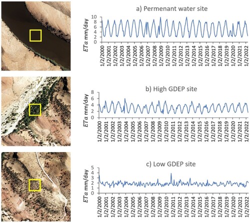
The process of water transfer to the atmosphere via ET is driven by several complex factors including temperature, humidity, wind speed, soil and plant type and water availability (Guerschman et al. 2022). In simplest terms, where temperatures are high and humidity is low (for dryer climates), and where there is water availability (either surface water or saturated soil/groundwater) ET will be much higher. This was evident in our study area for several high and low potential GDE locations assessed using the Google Earth Engine application ‘AET Explorer’ (TERN 2022) (Figure 3). While bias correction of the national CMRSET ET product is proposed for improved measurements of $E{T}_a$ (Doody et al. 2023), relative trends and differences between wet and dry periods was considered acceptable for analysis.

Figure 3. Temporal late dry period $E{T}_a$ relative to wet period $E{T}_a$ sample plots with corresponding aerial photo location for (a) permanent water, Aroona Dam (Figure 10(e)); (b) a high GDEP site, west of Aroona Dam (Figure 10(e)); and (c) a low GDEP site, south-west of Aroona Dam (Figure 10(e)).

Thus, the assumption was made that vegetated areas that exhibited higher $E{T}_a$ during late dry periods, relative to the wet, with little intermediate rainfall, may indicate consistency of water supply (SKM and CSIRO 2012, 92). The contrast is shown using a normalised difference $[E{T}_a]$index between the wet and late dry period measured $E{T}_a$, such that: (4) $NDE{T}_{a}I={\displaystyle \frac{E{T}_{aMeandry}-E{T}_{aMeanwet}}{E{T}_{aMeandry}+E{T}_{aMeanwet}},}$(4) where $E{T}_{aMeandry}$ and $E{T}_{aMeanwet}$ are the mean of the late dry and wet period $E{T}_a$ estimates, respectively, and where higher $NDE{T}_{a}I$ values closer to 1 (with a range −1 to +1) indicate areas of higher GDEP. The index range was standardised to values between 0 and 1 using equation (2).

2.7. Supporting geological factors – fractured rock aquifers

While focussing mainly on remote sensing-based physiological indicators, two locally relevant geological parameters were incorporated to assist GDE identification. According to the report by SKM and CSIRO (2012), which details the GDEP mapping rules of the nation-wide GDE Atlas, no datasets were used that distinguish fractured rock aquifers from unfractured aquifers in eco-hydrological zone 33 (EHZ33); within which this study area sits. Thus, all formations within the Adelaide Geosyncline were assumed to be fractured enough to allow baseflow to rivers. This study refines such broad-scale application by applying lithology and geo-lineament mapping methods undertaken in the Flinders Ranges by Fildes et al. (2020) who suggest faults in local crystalline rocks, may provide the only zones capable of groundwater flow. Thus, these zones may delineate specific areas with increased baseflow to rivers and localised groundwater access to the root zone.

Fieldwork was used to ground truth published lithology mapping classes (SARIG 2021a) and to rank relative importance based on primary and secondary porosity characteristics (Fildes et al. 2020) to gain a localised understanding of their potential to support groundwater-vegetation interactions (Table 3). Geo-lineaments were also mapped using 1:100 K and 1:2 M lineament datasets (SARIG 2021b, 2021c), along with photo-interpreted lineaments digitised from Google Earth imagery (< 50 cm resolution). Lineaments delineate areas or fault zones with high secondary porosity characteristics. Analysis by Fildes et al. (2020) showed bores closer to fault zones on average have a higher yield, with diminishing association observed up to 1.2 km away from larger Neoproterozoic–Ordovician faults in the southern Flinders Ranges. In this study, the relative importance of each lineament was defined by lineament length, where longer lineaments/faults are typically deeper and more pervasive (Díaz-Alcaide and Martínez-Santos 2019; Sander, Minor, and Chesley 1997), and ‘type’, where Neoproterozoic–Ordovician faults in this region are characterised by a wider and more transmissive fault zone (Fildes et al. 2020). Based on work by Fildes et al. (2020) and field observations at Leigh Creek, three raster grids representing ‘distance from lineaments’ were generated for three potential influential fault zone widths relative to lineament length and type (1,200, 240, and 120 m). As a complete hydrogeologic function of lineaments was unknown, professional judgment was used to derive a generalised linear diminishing score for each fault zone width based on distance from each lineament (Table 1). All three rasters were summed to yield a raster with scores ranging from 0 to 6.2 where high values indicate lineament intersections or where fault zones overlap. A zero (‘0’) was assigned to areas outside of fault zones. A final rescaled (standardised) ‘lineament zone’ raster was produced using equation (2), where 0 and 6.2 were used as the ${\chi }_{min}$ and ${\chi }_{max}$ values.

Table 1. Diminishing scores used to rank relative importance/influence of lineaments based on lineament type, their length and fault zone width, where scores diminish with increased distance from the lineament centre line in each fault zone.

Lineament type	Lineament length (m)	Fault zone width | Distance from centre line (m)	Diminishing ‘score’ from centre line to outer fault zone
1:100k and photo-interpreted	<500	120 | 60	1.2 to 1 (0.2 reduction every 30 m)
	>500	240 | 120	2 to 1.4 (0.2 reduction every 30 m)
Neoproterozoic–Ordovician faults (pervasive)	>1000 (all)	2400 | 1200	3 to 1.2 (0.2 reduction every 120 m)

2.8. Parameter weighting and calculation of GDE potential

Raster calculation of GDEP combined each standardised GDEP parameter using a weighted linear combination method (Malczewski 2000). Parameter weights were determined based on their relative importance using the analytic hierarchy process (AHP) (Saaty 1977). The AHP is a structured weighting approach that minimises the challenges of weighting multiple criteria simultaneously. The AHP has been extensively used in spatial multi-criteria decision analysis (Dos Santos et al. 2019) and frequently used, along with the weighted linear combination, in groundwater potential mapping research (Díaz-Alcaide and Martínez-Santos 2019). The AHP comprises participant/expert-based pairwise comparisons between criteria using a numerical scale to yield a matrix of comparisons. Final criteria weightings are the normalised values, summed to 1, of the priority vector (eigenvector) determined from the row means of the comparison matrix. A consistency ratio (CR) is also produced to ensure criteria relationships are logically related rather than being randomly chosen (Saaty 1977, 237). A CR of < 0.10, or 10%, is considered an acceptable level of constancy, with a CR > 0.10 requiring re-evaluation of criterion pairs. While the AHP will not eliminate expert biases, it does provide a structured approach enabling a higher degree of evaluation of one’s choices, along with closer engagement and moderation between expert opinions.

Two key factors were considered in determining relative importance of each GDEP parameter. The first considered only the rationale of the parameter as an indicator of GDEP (e.g. changes in relative greenness vs changes in relative wetness). The second considered confidence in the spatial model and output representation of the rationale (e.g. NDCVI_NDVI vs TCW percentiles). For example, some modelled GDE parameters may exhibit ‘false positives’ due to spatial data limitations or susceptibility to terrain effects caused by seasonal differences in sun-angle.

With AHP derived weights for each parameter (Table 2), GDEP was calculated using: (5) $GDEP=\sum _j(w_j\times x_{ij})$(5) where w_j is the normalised AHP weight of the j-th parameter, and x_i is the i-th standardised value or class (weight) (0–1) of the j-th parameter for each alternative grid cell location. The weighted linear combination produced a final standardised range of values between 0 and 1 representing GDEP per grid cell over the study area, where 0 indicates no GDEP and 1 indicates maximum GDEP.

Table 2. Pairwise comparison matrix (showing relative importance based on consensus from authors), corresponding parameter AHP weights (w) and consistency ratio.

Parameters	1	2	3	4	5	6	7	Normalised Eigen values (w)
(1) NDCVINDVI	1	1/2	1	3	3	7	5	0.213
(2) NDCVIPVFC	2	1	2	3	3	7	5	0.290
(3) LBENDVI	1	1/2	1	3	3	7	6	0.218
(4) TCW	1/3	1/3	1/3	1	1	7	5	0.109
(5) $E{T}_a$	1/3	1/3	1/3	1	1	7	5	0.109
(6) Lineaments	1/7	1/7	1/7	1/7	1/7	1	1/3	0.023
(7) Lithology	1/5	1/5	1/6	1/5	1/5	3	1	0.039
Consistency ratio: 0.078

Importance	Definition	Explanation
1	Equal importance	Two elements contribute equally to the objective
3	Moderate importance	Experience and judgment slightly favour one element over another
5	Strong importance	Experience and judgment strongly favour one element over another
7	Very strong importance	One element is favoured very strongly over another
9	Extreme importance	The evidence favouring one element over another is of the highest possible order of affirmation
2, 4, 6, 8 can be used to express intermediate values
Reciprocal values show inverse comparison

Definition and explanation descriptions adapted from Goepel (2013). Note there was no parameter judged to have ‘extreme importance’ (‘9’) over another.

2.9. Model validation

Direct methods of validation, such as pre-dawn leaf water potentials, isotope analysis, environmental or introduced tracers were beyond the scope of this study. Alternatively, GDEP mapping results were compared against known spring locations, and likely root depth of vegetation with depth to groundwater (DGW) as a form of validation (Canadell et al. 1996). An ‘inferred’ DGW surface was prepared by subtracting a reduced standing water level surface, derived from an inverse distance weighted network of recent and historical bores (2,716), from a digital elevation model (DEM). The 1 arc-sec Shuttle Radar Topography Mission (SRTM) DEM-S (smoothed) product was used for improved vertical accuracy (GA 2011). The inferred DGW surface was then overlaid with final GDEP mapping results as well as a detailed floristic vegetation map. Likely root depth was attributed to key species based on literature, and validation of vegetation types supported by field observation. A general comparison was also made between derived GDEP mapping results and corresponding areas presented in the national GDE Atlas (Doody et al. 2017; BAP 2016).

3. Results

3.1. Parameter weighting results

A consensus on pairwise GDEP parameter comparisons (and thus their final weights) was achieved by five experts, consisting of two senior geospatial scientists, two senior geospatial eco-hydrogeologists, and a senior geologist/hydrogeologist, all with extensive experience and knowledge of the remote study area (Table 2).

The AHP method of weighting was not only used to derive ‘global’ weights for each GDEP parameter, but also to derive weights for each lithology class (Table 3).

Table 3. Lithology classes and their corresponding normalised and standardised weights (x) that reflect their relative importance determined using the AHP, facilitated through expert elicitation of pairwise class comparisons.

Lithology class	Normalised weight	Standardised weight (x)
Alluvium	0.474	1
Sandstone	0.275	0.580
Shale, Siltstone	0.169	0.357
Limestone, Dolomite	0.051	0.108
Quartzite	0.032	0.068

Note the standardised lithology class weights (x) were used in the final weighted linear combined GDEP calculation (Equation (5)).

3.2. GDEP mapping results

Mapping results include individual maps for each contributing GDEP parameter (Figures 4–9) and a final combined GDEP map (Figure 10). The subset locations, a–h, in each figure were chosen as ‘control’ to evaluate behaviour of the individual modelled parameters where a higher likelihood of groundwater-vegetation interaction might occur, largely due to a relatively shallow DGW and presence of local phreatophyte species such as E. camaldulensis and M. glomerata. Modelled GDEP in these locations were also compared with GDE Atlas outputs.

Figure 4. Results of the NDCVI_NDVI greenness parameter, showing: (a–h) model ‘control’ locations where GDEP was expected to be high (with corresponding high-resolution image); and (i) the spatial distribution of NDCVI_NDVI indicator mapping results over the study area and the location of each subset.

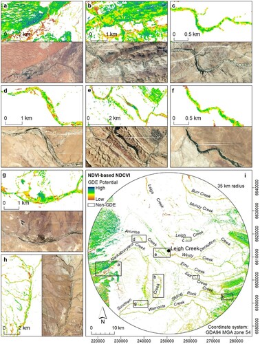
Figure 5. Results of the Barest Earth greenness parameter, showing: (a–h) model ‘control’ locations where GDEP was expected to be high (with corresponding high-resolution image); and (i) the spatial distribution of the Barest Earth greenness parameter mapping results over the study area and the location of each subset.

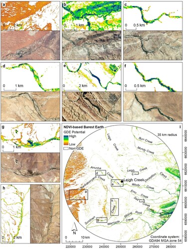
Figure 6. Results of the NDCVI_PVFC cover parameter, showing: (a–h) model ‘control’ locations where GDEP was expected to be high (with corresponding high-resolution image); and (i) the spatial distribution of the NDCVI_PVFC cover parameter mapping results over the study area and the location of each subset.

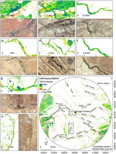
Figure 7. Results of the TCW 10th percentile (wetness) parameter, showing: (a–h) model ‘control’ locations where GDEP was expected to be high (with corresponding high-resolution image); and (i) the spatial distribution of the TCW 10th percentile (wetness) parameter mapping results over the study area and the location of each subset.

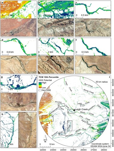
Figure 8. Results of the $E{T}_a$ (wetness) parameter, showing: (a–h) model ‘control’ locations where GDEP was expected to be high (with corresponding high-resolution image); and (i) the spatial distribution of the $E{T}_a$ (wetness) parameter mapping results over the study area and the location of each subset.

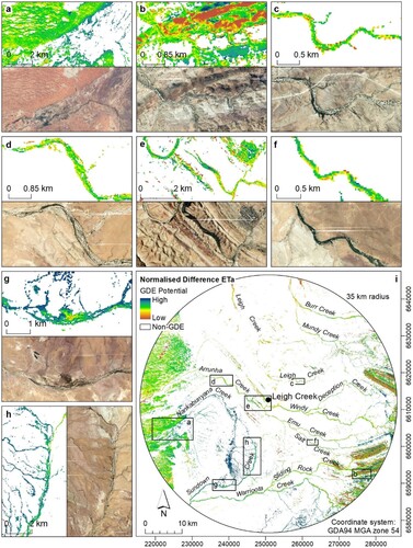
Figure 9. Lithology and lineament (fault zone) parameters, showing: (a–h) subset areas with corresponding higher resolution image for comparison with areas shown in Figures 4–8; and (i) the spatial distribution of lithology and fault zones over the study area and the location of each subset.

Figure 10. Final combined GDEP mapping results overlaid with inferred DGW surface for pseudo validation. Subset areas a–h showing larger-scale areas as indicated in the main map (i). Note, inferred DGW areas with negative depths (<0 m, pink through purple areas) were interpolated to have a DGW higher than the ground level. This was largely due to the absence of bore data in these lower lying areas. However, they are likely to be areas of consistently shallow DGW, as indicated by their shallow DGW surrounds.

3.2.1. Individual parameter mapping results

Qualitative inspection of each contributing parameter indicates similarities in GDEP mapping results, though key differences are apparent (Figures 4–9). For example, contrasting GDEP is evident between the two greenness parameters, NDCVI_NDVI (Figure 4) and LBE_NDVI (Figure 5), most noticeable in the west of the study area. Subset (a) in both figures reveal good agreement in low GDEP within the central diagonal running floodout consisting of Holocene alluvial/fluvial sediments dominated by Acacia victoriae over mixed chenopod species (DEW 2022). However, contrasting GDEP is shown over the adjacent north and south sandy dunes and plains consisting largely of Casuarina pauper low open woodland over Acacia ligulata shrubland and Senna artemisioides ssp. petiolaris low sparse shrubland (DEW 2022). There is generally good agreement between these two greenness parameters over the broader study area, however, as shown in subsets b–g, the LBE_NDVI parameter exhibits clear ‘pockets’ of much higher relative GDEP compared with the NDCVI_NDVI results. Field observations confirm many of these locations consist of relatively dense and tall (> 6 m) M. glomerata, typically located along creeks, which are known groundwater users (Brim Box et al. 2022; CDM Smith 2020).

The NDCVI_PVFC mapping results (Figure 6), largely correspond with the spatial distribution of the NDCVI_NDVI results (Figure 4). Though overall, observed is a greater contrast in the NDCVI_PVFC results over the study area. Excluding subset (a), pockets of higher relative NDCVI_NDVI GDEP are more aligned with the higher GDEP areas mapped by the LBE_NDVI parameter (Figure 5), largely along stream channels and adjacent floodout/terraced areas dominated by M. glomerata and more broadly, E. camaldulensis.

Inspection of the two wetness parameters, TCW and $E{T}_a$ (Figure 7 and 8), again show similarities in GDEP results, particularly within the creeks and floodout areas. However, mostly moderate levels of GDEP with lower spatial variation dominated the $E{T}_a$ mapping results compared with the TCW and clear differences in spatial variation are observed in subsets a, b and g. Overall, GDEP variation was noticeably higher for the TCW results, which aligned well with the greenness and fractional cover GDEP mapping (Figures 4–6), while the sand dunes/sandy plains in the north-west of Figure 7(a), largely concurred with the very low GDEP results of the LBE_NDVI. The latter was expected given both the LBE_NDVI and TCW 10th percentile models were derived from higher-frequency sampling over a longer time-period, thus both suggesting that at some point in time, vegetation greenness and wetness was very low over this landform and access to groundwater was unlikely. Conversely, the spatial variation in the $NDE{T}_{a}I$ results were more aligned with parameters that also used targeted inter-seasonal date pairs (excluding subset b).

The mapped fault zones (Figure 9) largely coincide with classes of lithology (Table 3) that typically exhibit lower primary porosity characteristics, potentially increasing their influence to allow access to groundwater. Though the lower weighting of lineaments and lithology will only slightly moderate the results of the combined vegetation parameters.

3.2.2. Final GDEP mapping results

The final combined ‘multiple-lines-of-evidence’ GDEP mapping of the study area reflects the sum of all GDEP parameters, their rationale and spatial representation, moderated by their relative importance using weights determined by the AHP (Figure 10). Figure 10 also shows the distribution of GDEP in association with the inferred DGW surface to aid map result validation. Qualitatively, overall observations demonstrate good agreement between higher GDEP mapped areas and shallow DGW.

For comparing results with the GDE Atlas, the derived GDEP index range (0.18–0.91) was first classified into five equal interval discrete class levels using a four standard deviation min–max range to minimise the influence of outliers on the lower- and higher-end class range (Table 4). While the qualitative GDEP levels in the GDE Atlas were derived using a normalised weighting and expert elicitation approach (Doody et al. 2017), the derived GDEP discrete class levels in this study are comparable in a qualitative sense and allow quantification of mapping results for each class. Notably, of the 3848 km² study area, 87.5% was considered to have no GDEP as a result of applying the mean late dry NDVI and LBE_NDVI thresholds (< 0.15), along with the mean late dry PVFC threshold (< 10%). Of the remaining 12.5% (482 km²), Table 4 lists the relative % and area in km² for each GDEP class, with a large percentage of moderate GDEP illustrated, a reflection of the equal interval classification with a normal distribution dataset.

Table 4. Class ranges that define the qualitative GDEP class levels.

Class no.	GDEP description	Class ranges	Area & % of PV areas
1	Very low	0.18–0.35	8.24 km^2 (1.71%)
2	Low	0.35–0.45	80.31 km^2 (16.67%)
3	Moderate	0.45–0.56	305.27 km^2 (63.37%)
4	High	0.56–0.67	83.61 km^2 (17.36%)
5	Very high	> 0.67	4.31 km^2 (0.89%)

Note class ranges determined using an equal interval range between the min-max values defined by applying a 4 SD measure to the GDEP results to remove the influence of outlier values as shown in the table histogram.

A comparison is provided between ‘derived’ GDEP mapping classes and those defined by the GDE Atlas for 27 corresponding landform type locations in each subset area, along with the dominant vegetation species, their phreatophyte status and rooting depth (Table A1). Of the 15 locations listed in Table A1 with ≥ ‘high’ derived GDEP, 13 (86.7%) coincided with known GDE species and favourable DGW (locations 3, 5–7, 9, 10, 14–16, 19, 20, 24, 26). For all 27 locations, 19 (70.4%) (darker blue rows) were observed to have strong agreement between derived GDEP and corresponding site conditions, while 12 (44.4%) strongly agreed with the GDE Atlas (green rows), eight (29.6%) moderately agreed (yellow rows), and seven (26%) with a weak agreement (orange rows).

Further GDEP model validation using 34 known spring locations within the study area, revealed a high level of model reliability (Figure 11). Of the 34 springs, 26 (76.5%) coincided with ≥ ‘high’ GDEP, three (8.8%) with ‘moderate’ GDEP, and three (8.8%) with ‘low’ GDEP, while only two spring locations (5.9%) were observed to have no GDEP.

Figure 11. Maximum GDEP within 100 m of known spring locations, where each spring is also classified by its qualitative GDEP class level. Dark blue = ‘very high’ (> 0.67), dark green = ‘high’ (0.55–0.67), bright green = ‘moderate’ (0.45–0.55), and orange = ‘low’ (0.35–0.45). There were no springs coinciding with a ‘very low’ class level (< 0.35). Note: GDEP within 100 m was chosen to account for seepage from source and scale-relevant positional accuracy. Source: Ecosystem Type ‘Spring’ from Aquatic GDEs layer (BAP 2016).

4. Discussion

4.1. Individual parameter contributions

The performance of each contributing parameter is discussed in context of its assigned weighting, largely determined by the confidence in its rationale for inclusion and apparent performance of its modelled spatial representation, specific to this arid landscape. Each input parameter provided complementary rather than duplicative physiological traits in response to prolonged dry periods.

4.1.1. Greenness parameters

The NDCVI_NDVI model captured wet versus late dry response for targeted dates, while the LBE_NDVI captured landscape response from higher-temporal inter-seasonal contiguous sampling over a much longer period. The latter model is most analogous to recording the ‘minimum’ NDVI value for each grid cell over a long contiguous time-period and thus may be more attuned to capturing groundwater obligate species where greenness persists (very high GDEP). Conversely, the very low GDEP areas derived by the LBE_NDVI suggests that at some point during the contiguous sampling of images, these areas were very dry, exhibiting little greenness (e.g. Figure 5(a)). Thus, both models appear complementary where the LBE_NDVI has identified ‘hot spots’ of possible obligate GDEs, while the moderate to high GDEP values identified by the NDCVI_NDVI model may have identified more disconnected GDEs which rely on groundwater intermittently. Consequently, the final normalised AHP derived weighting for both greenness models were almost identical (Table 2) and were assigned two of the three highest weightings.

Notably, a benefit of the CV-based NDCVI is that it normalises the measure of persistency for differences in green vegetation cover, even at very low cover levels where vegetation may still be accessing groundwater to some degree during prolonged dry periods. For example, deep rooted E. camaldulensis (river red gums) are known users of groundwater (Doody et al. 2014, 2015), yet they only sparsely populate creek beds. Despite a large crown diameter and open canopy, they may only have a foliage projected cover occupying 20% of a 30 × 30 m Landsat pixel yielding a lower NDVI or green signature. Where the SD statistic of the CV/NDCVI calculation is comparative proportionally to different parameter mean values such as different cover/density levels, it will yield the same or similar CV/NDCVI value, making it well suited to mapping persistency in low cover heterogeneous landscapes such as semi-arid/arid environments, while working equally well in heavily vegetated areas.

4.1.2. Fractional cover parameter

The NDCVI_PVFC model shares the same beneficial properties as that of the NDCVI_NDVI model. In addition, fractional cover has been proposed as a preferred indicator of landscape condition in semi-arid environments where plant density and foliage projective cover are low (Scarth, Röder, and Schmidt 2010; Graetz, Pech, and Davis 1988), and where greenness indices (e.g. NDVI) may perform poorly in sparsely vegetated areas due to the influence of the bright soil and plant litter background signal. Comparing mean NDVI and mean PVFC indices (Figure S1) supports this assessment. Thus, the ability to map PVFC variations at ≤ 20%, per grid cell, is significant in estimating the persistency of low cover/singular trees, which may have access to groundwater. Although the rationale for mapping the persistency of both vegetation greenness and cover were considered equally important, the NDCVI_PVFC model was given the highest normalised AHP weighting (Table 2) due to its ability to map changes in low PVFC in areas where changes in NDVI were indistinguishable.

4.1.3. Wetness parameters

While the orthogonality of the TCW index ensures less interaction with its companion tasselled cap trajectories of soil brightness and vegetation greenness, it is still suspectable to variations in underlying soil/lithology colour, which may cause misleading results. This is most noticeable to the west of the subset (h) boundary drawn in Figure 7(i). This north–south running Acacia aptaneura woodland exhibited variations in moderate to high TCW values. The area largely consists of dark red silcrete gibber, which has lowered the contrast between NIR and SWIR reflectance, artificially increasing the level of apparent wetness relative to the surrounding lithologies. Moreover, the standardisation of the TCW 10th percentile min–max values between 0 and 1, is another potential model limitation, which is only valid for this study area. Hence, while the rationale for mapping persistency of vegetation wetness was considered significant, the TCW 10th percentile model was judged to yield a lower relative normalised AHP weight (Table 2), which largely reflected these limitations.

An alternate measure of vegetation wetness persistency was derived using the $NDE{T}_{a}I$ model (Figure 8). As a normalised difference measure, the model normalises for differences in vegetation cover (and sub-pixel content) with respect to mean wet versus mean late dry relative differences in $E{T}_a$. Like the two NDCVI models, this is an important model trait, ensuring vegetation species that may be consistently accessing groundwater yet only occupy a small area of a grid cell or have a lower foliage projected cover/open canopy (such as sparsely spaced E. camaldulensis), calculate to a higher GDEP index value.

However, the $NDE{T}_{a}I$ model output was observed to be susceptible to topographic shadowing, most noticeable on south facing hill slopes and in valleys where high contrasting very low GDEP was evident (yellow–orange areas in Figure 8(b)). Topographic shadowing reduces NIR and, to a larger degree, SWIR reflectance. Spectral indices that use these wavelengths like the global vegetation moisture index (GVMI) (Ceccato, Flasse, and Grégoire 2002) used in the $E{T}_a$ calculation, may be biased towards higher wetness or moisture index values in topographic shadowed areas where these areas share similar spectral characteristics with water in optical images (Huang et al. 2018). Despite the use of the NBART Landsat product to reduce topographic variation, the $NDE{T}_{a}I$ model highlighted this contrast where significantly higher $E{T}_a$ was measured in terrain shadowed vegetated areas during winter months compared with much lower $E{T}_a$ during the summer months resulting in very low GDEP as determined by the $NDE{T}_{a}I$. Indeed, a reversal of this response would be expected if vegetation in these areas were accessing groundwater, which could not be confirmed. Nevertheless, the $NDE{T}_{a}I$ results behaved as expected in areas not affected by topographic shadowing, clearly showing areas which largely corresponded with GDEP as measured by other parameters. Considering these limitations, the $E{T}_a$ parameter was judged to have the same relative normalised AHP weight as the TCW 10th percentile parameter (Table 2).

4.1.4. Lineaments and lithology parameters

While these geological factors may be significant in this fractured rock eco-hydrological zone (EHZ33) (SKM and CSIRO 2012), their relative influence is implied rather than measured directly. The primary and secondary porosity characteristics for each lithology class was assessed through field observations and measurements at sample/representative sites only. Thus, an assumption of uniformity is applied more broadly across each lithology class (polygon), which does not consider the variation within a unit (Fildes et al. 2022). Moreover, the relative influence of fault zones was estimated from work adapted from Fildes et al. (2020), though their actual influence is unknown and only an indirect/inferred level of importance was applied. Consequently, the two geological parameters were assigned the lowest normalised AHP weightings (Table 2).

4.2. Overall model performance and efficiency

Final GDEP mapping results reflected the combined weighted performance of each parameter output (Figure 10). Each exhibited more overall strengths than weaknesses thus maximising model performance in a multiple-lines-of-evidence context. Comparing final mapping results with independent GDEP indicators demonstrated a reliable mapping approach (Section 3.2), aiding in the identification and spatial variability in potential groundwater use by different vegetation types which cannot otherwise be easily determined. For example, as a known groundwater user, M. glomerata may be visibly pronounced in dry season high-resolution aerial photography though in some areas it may exhibit a much lower GDEP than near-by less visibly green vegetation such as E. camaldulensis (Figure 12).

Figure 12. High-resolution aerial photograph (middle) showing a dense and prominent line of M. glomerata (inland paperbark) on the western side of Arrunha Creek (grey arrows). The GDEP mapping results (top) exhibit a much higher relative GDEP in the middle and on the eastern side of the creek bed (black arrows), corresponding with more sparsely vegetated and less prominent E. camaldulensis (river red gum) as observed in the aerial photograph. Terrestrial photograph (bottom) showing E. camaldulensis and M. glomerata in a similar setting in the same study area taken just south of Aroona Dam.

While the GDEP model consists of multiple input parameters, each was developed to minimise the technical overheads often required in more complex image analysis-based GDEP persistency models. Alternative remote sensing approaches can incur a higher degree of image analysis expertise to derive reliable results. For example, Castellazzi, Doody, and Peeters (2019) utilised multi-temporal InSAR,⁴ Barron et al. (2014) used scene dependent unsupervised classification methods and Martínez-Santos et al. (2021) used supervised machine learning, with all methods requiring differing but considerable image analysis expertise.

One of the benefits of the GDEP model is that it is largely user independent. Only relevant wet and prolonged dry period response dates are required for download of the necessary open-access datasets. The model requires only the calculation of routine temporal image statistics for input to the NDCVI and ND$E{T}_a$I model and their standardisation with the LBE_NDVI and TCW indices before aggregation to yield a final composite GDEP index. Only variations in parameter weights will affect model output differences between users where the AHP may require a degree of expert-knowledge input, though its design aims to provide a straightforward structured process (Saaty 1977). Importantly, the AHP enabled a systematic assessment of the rationale, spatial representation, and modelled output behaviour of each input parameter to be considered. Consequently, in future studies, a structured weighting approach, such as the AHP, would be encouraged as part of a broader participatory multi-criteria evaluation by which decision-makers attain a deeper understanding of the model structure and behaviour. This would help to mitigate duplication between input parameters with a goal to improve GDEP mapping results, which is not well justified in the GDEP mapping literature.

Finally, the novel application of the CV statistic combines both mean parameter index values with SD measures, which would otherwise be treated as separate criteria (e.g. Xu et al. 2022) in a normalised difference model (NDCVI). Like the $NDE{T}_{a}I$, the NDCVI accounts for spatial variations in vegetation cover (including sub-pixel content) making them more practical in complex/heterogeneous landscapes. The NDCVI may also perturb other alternate input parameters, such as wetness or moisture indices. The availability of Landsat-scale national data products used for all index-based parameter evaluations, will also help facilitate the model’s broader application, particularly where there is flexibility in the number of input parameters that might be used. For example, the NDCVI_PVFC and LBE_NDVI were judged to be the most robust input parameters (targeted intra-annual prolonged dry periods versus higher temporal and longer-term analysis, respectively). These two parameters alone might be combined (perhaps using equal weighting) as an initial ‘first run’ analysis to identify potential GDEs. Otherwise, a ‘full set’ of parameters may be combined, moderated by their relative weights, to refine/improve model performance. Either approach could be used as an independent analysis, or they might be incorporated into a broader zonal/topographic GDEP parameter rule-set (e.g. Duran-Llacer et al. 2022; Martínez-Santos et al. 2021) targeting specific eco-hydrological zones, such as those defined in the national GDE Atlas of Australia or other applications utilising continental scale remote sensing data sets (e.g. Digital Earth Africa).

4.3. Limitations

4.3.1. General model limitations

Arid vegetation species are well-adapted to periods of water deficit. Thus, the GDEP model may produce false positive results indicating groundwater dependency with species that are simply well-adapted to drought. However, while these may include larger perennial trees, they are more likely to be xeric chenopod species; the areas of which have been removed by the NDVI (< 0.15) and fractional cover (< 10%) masks leaving primarily ‘green’ vegetation, which rely on more frequent rainfall events or have some access to groundwater.

The GDEP model is more likely to produce false negative results due to the combined/mixed signal response of diminishing greenness and cover of understory plants during prolonged dry periods, unrelated to the relative persistency of its overstory (Eamus et al. 2015). Overgrazing of shrubs and grasses from feral animals and domestic stock during these periods can also be significant contributors to the vulnerability of rangeland health (Bastin, Tynan, and Chewings 1998; Pickup and Chewings 1994). Nevertheless, a typical understory of Triodia, Atriplex, Mariana and Sclerolaena species was observed for E. camaldulensis woodlands, which dominate stream beds, and nearby floodouts and terraces throughout the study area. These companion understory plants are likely subject to grazing and drought pressures, yet these areas exhibited a relatively high derived GDEP reflecting the water requirements of E. camaldulensis, which often require access to groundwater to supplement their needs (Doody et al. 2014, 2015). Largely, their occurrence throughout the study area coincided with relatively shallow DGW conducive to groundwater access. Thus, despite its limitations, the reliability of the GDEP model appears to have performed well in these woodland areas. This is also true for areas dominated by M. glomerata, found on terraced areas within and adjacent streams, which often yield the highest GDEP values; particularly where higher density groves mask the behaviour of their understory.

4.3.2. Model validation limitations

Several factors limit comparisons between GDEP mapping results and site conditions (Table A1), including actual rooting depth, which can be highly variable (Cook and Eamus 2018); a DGW that is only ‘inferred’; and fluctuations in groundwater levels as a response to local rainfall and recharge rates (Somaratne 2019). Nevertheless, the summary of comparisons is considered reliable, which take into account likely error in DGW surface generation, particularly in lower lying areas where bore data was sparse. These areas were mapped as having a negative DGW based on higher reduced standing water level bore measurements obtained from higher surrounding elevations. Thus, such lower lying areas are more likely to have a shallow DGW allowing roots to access groundwater.

Only general comparisons could be made between GDEP mapping results and corresponding locations in the GDE Atlas, mainly due to differences in the underlying source data resolutions and aggregation methods between each modelling approach. Other than the inflow-dependent ecosystem layer (Doody et al. 2017; van Dijk et al. 2015), GDEP in the GDE Atlas is assigned to broader-scale vegetation community polygons and river/wetland polygons for terrestrial and aquatic GDEs, respectively, based on a ‘majority value’ rule for factor contributions (Doody et al. 2017; SKM and CSIRO 2012). Thus, smaller areas of high GDEP mapped in this study will be underrepresented in the GDE Atlas, resulting in lower comparative agreement. While acknowledging these limitations, where ‘direct’ comparisons can be made between spring locations and derived GDEP, along with locations having conditions and species conducive to groundwater uptake, overall, the results suggest a reliable GDEP model.

4.4. Future implications for groundwater exploration around Leigh Creek

While prioritising areas for future groundwater exploration efforts is beyond the scope of this study, the GDEP modelling results highlight areas where further on-ground investigations are required to evaluate their GDE status and possible protection from future groundwater development. These areas fall within 10 km of the Leigh Creek desalination plant (the prescribed zone limiting groundwater development). Areas within this zone mainly include Arrunha, Windy, Emu and Leigh Creeks, which exhibited variations of moderate to high GDEP with some localised areas exhibiting very high GDEP (Figure 10(i) and subsets c–f). The area is dominated by fractured rock aquifers. A high yielding bore located just south of where both Windy and Emu Creeks join to flow into Aroona Dam (Figure 9(e)) is thought to be fed by the large north-west to south-east running pervasive fault zone (pers comm. hydrogeologists Nara Somaratne and Ian Clark, field observations, Leigh Creek, November 09, 2020). This highly fractured area is likely providing pathways for groundwater movement and storage along several adjoining formations. Any assessment of the vulnerability of GDEs in this region would need to consider these highly variable and complex geological variations where siting new bores near GDEs [may or] may not have a direct impact on them. Conversely, bores sited further away may have an impact depending on an analysis of their connectivity.

Regarding the management of existing bores, there are currently seven operational town water supply bores located along Windy and Emu Creeks. The water from each is ‘blended’ to lower their salinity level to meet the operational requirements of the desalination plant process (Somaratne 2019). The derived GDEP maps will help target areas for more detailed hydrogeological analysis and could form part of a broader decision-making metrics for decommissioning bores or prioritising the [re]ordering of bores for blending to help protect sensitive ecosystems.

5. Conclusions

Protection of GDEs first requires their identification, however their use of groundwater is largely hidden beneath the ground. This research developed a straightforward, yet effective remote sensing-based GDE mapping approach based on the persistency of vegetation parameters to indicate the relative drying of vegetation during prolonged dry periods, inferring their potential relative dependency on groundwater. The approach is best suited to climatic areas with distinct prolonged dry periods, such as the large arid and semi-arid regions of Australia employing high-resolution (Landsat) image derived products at a national scale. The approach is also likely to be applicable to other continental Earth observation data cubes which utilise analysis-ready data and have the capacity to generate products such as barest Earth, fractional cover, wetness percentiles and actual evapotranspiration. Moreover, the mapping approach complements the growing number of groundwater potential mapping studies, which often do not apply spatial constraints on where groundwater abstraction should be avoided to protect sensitive GDEs. Though the GDEP model’s applicability to other climatic landscapes and eco-hydrological zones would require further validation.

With the addition of two geological parameters, each vegetation parameter was ‘objectively’ combined to produce an index of GDE potential (GDEP) from which targeted on-ground investigations can confirm the phreatophyte status of vegetation, thus aiding in the understanding of local groundwater regimes and GDE requirements. This information will help regional managers facilitate the protection of GDEs and their integration into water resource management plans.

Acknowledgments

This work was supported by an Australian Government Research Training Program Scholarship, and a Commonwealth Scientific and Industrial Research Organisation (CSIRO) Top-up Scholarship. The authors give their appreciation to the organisations cited throughout this manuscript for the open-access data upon which this research was conducted. We also thank the four anonymous reviewers for their valuable feedback.

Disclosure statement

No potential conflict of interest was reported by the author(s).

Data availability statement

Baseline datasets generated by Geoscience Australia (NBART surface reflectance, fractional cover, barest Earth, wetness percentiles), Terrestrial Ecosystem Research Network (TERN) (Actual Evapotranspiration), and the Bioregional Assessment Programme (National GDE Atlas data) are available as cited throughout the manuscript. Derived data supporting the findings of this study are available from the corresponding author, S. G. Fildes, upon reasonable request.

Correction Statement

This article has been corrected with minor changes. These changes do not impact the academic content of the article.

Notes

1 Commonwealth Science and Industrial Research Organisation.

2 MODerate resolution Imaging Spectroradiometer.

3 Visible Infrared Imaging Radiometer Suite.

4 Interferometric Synthetic Aperture Radar.

Appendix A

Table A1. Summary of derived GDEP for each subset/control location (a–h) relative to the GDEP as designated by the GDE Atlas and site conditions.

Derived GDEP and the GDE Atlas results are compared using subjective GDEP class levels (derived from different methods), where the GDE Atlas potential is also denoted with either an ‘A’ or ‘T’ superscript identifying its source as either an Aquatic or Terrestrial GDE, along with its corresponding inflow-dependent ecosystem (IDE) level. For example, higher IDE indicates higher GDEP where ET exceeds rainfall (van Dijk et al. 2015). For the derived GDEP, a sampled index value range is provided for each corresponding location. Cell colour represents agreement between the two datasets: Green = strong agreement, Yellow = moderate agreement, Orange = weak agreement. For each subset, Landforms and Dominant species are included, with their likely phreatophyte status and rooting depths (based on literature) for comparison with corresponding derived DGW and GDEP at each location. Cell colour represents agreement between derived GDEP and the potential for plants to access groundwater as per the dominant species, phreatophyte status, rooting depth and DGW: Dark blue = higher agreement, and light blue = lower agreement.

¹ Doody et al. (2015); ²Doody, Hancock, and Pritchard (2018); ³CDM Smith (2020); ⁴Cook and Eamus (2018); ⁵Orellana et al. (2012); ⁶QG (2015); ⁷SKM (2010). Full reference description in main text. ⁹Species previously known as Acacia aneura.

References

- Alcoe, Darren, and Volmer Berens. 2011. Non-Prescribed Groundwater Resources Assessment – Northern and Yorke Natural Resources Management Region. Phase 1 – Literature and Data Review. DFW Technical Report 2011/17. Adelaide: Department for Water, Government of South Australia.
- Alharbi, Saif, William R. Raun, Daryl B. Arnall, and Hailin Zhang. 2019. “Prediction of Maize (Zea mays L.) Population Using Normalized-Difference Vegetative Index (NDVI) and Coefficient of Variation (CV).” Journal of Plant Nutrition 42 (6): 673–6799. doi:10.1080/01904167.2019.1568465.
- BAP (Bioregional Assessment Programme). 2016. “National Groundwater Dependent Ecosystems (GDE) Atlas. Bioregional Assessment Derived Dataset.” Accessed 5 May 2022. http://data.bioregionalassessments.gov.au/dataset/e358e0c8-7b83-4179-b321-3b4b70df857d.
- Barron, Olga V., Irina Emelyanova, Thomas G. Van Niel, Daniel Pollock, and Geoff Hodgson. 2014. “Mapping Groundwater-Dependent Ecosystems Using Remote Sensing Measures of Vegetation and Moisture Dynamics.” Hydrological Processes 28 (2): 372–385. doi:10.1002/hyp.9609.
- Bastin, G. N., R. W. Tynan, and V. H. Chewings. 1998. “Implementing Satellite-Based Grazing Gradient Methods for Rangeland Assessment in South Australia.” Rangeland Journal 20 (1): 61–76. doi:10.1071/RJ9980061.
- Bierkens, Marc F. P., and Yoshihide Wada. 2019. “Non-Renewable Groundwater Use and Groundwater Depletion: A Review.” Environmental Research Letters 14: 6. doi:10.1088/1748-9326/ab1a5f.
- BoM (Bureau of Meteorology). 2021. Climate Statistics for Australian Locations. Summary statistics Leigh Creek Airport SA (017110). Australian Government. Accessed 5 March 2021. http://www.bom.gov.au/climate/data/index.shtml.
- Brim Box, Jayne, Ian Leiper, Catherine Nano, Danielle Stokeld, Peter Jobson, Adrian Tomlinson, Dale Cobban, et al. 2022. “Mapping Terrestrial Groundwater-Dependent Ecosystems in Arid Australia Using Landsat-8 Time-Series Data and Singular Value Decomposition.” Remote Sensing in Ecology and Conservation. doi:10.1002/rse2.254.
- Canadell, J., R. B. Jackson, J. B. Ehleringer, H. A. Mooney, O. E. Sala, and E.-D. Schulze. 1996. “Maximum Rooting Depth of Vegetation Types at the Global Scale.” Oecologia 108 (4): 583–595. doi:10.1007/BF00329030.
- Castellazzi, Pascal, Tanya M. Doody, and Luk Peeters. 2019. “Towards Monitoring Groundwater-Dependent Ecosystems Using Synthetic Aperture Radar Imagery.” Hydrological Processes 33 (25): 3239–3250. doi:10.1002/hyp.13570.
- CDM (Camp, Dresser and McKee) Smith. 2020. “West Musgrave Project (WMP) Pre-Feasibility Study – Appendix A. Assessment of Potential Groundwater Dependent Ecosystems in the West Musgrave Project Area.” Report for OZ Minerals Exploration Pty Ltd. 18 March 2020. In Appendix B2. Assessment of Potential Groundwater Dependent Ecosystems. West Musgrave Copper and Nickel Project EPA Section 38 Referral Supporting Document. West Perth, WA.
- Ceccato, Pietro, Stéphane Flasse, and Jean-Marie Grégoire. 2002. “Designing a Spectral Index to Estimate Vegetation Water Content From Remote Sensing Data Part 2. Validation and Applications.” Remote Sensing of Environment 82 (2–3): 198–207. doi:10.1016/S0034-4257(02)00036-6.
- Chanda, Saoli, Yumiko Kanke, Marilyn Dalen, Jeffrey Hoy, and Brenda Tubana. 2018. “Coefficient of Variation From Vegetation Index for Sugarcane Population and Stalk Evaluation.” Agrosystems, Geosciences & Environment 1 (1): 1–9. doi:10.2134/age2018.07.0016.
- Chen, Yun, Jia Yu, and Shahbaz Khan. 2013. “The Spatial Framework for Weight Sensitivity Analysis in AHP-Based Multi-Criteria Decision Making.” Environmental Modelling & Software 48: 129–140. doi:10.1016/j.envsoft.2013.06.010.
- Clark, Ian, and Lynn Brake. 2008. “Sustainable Management of Groundwater Resources in Parts of Arid South Australia.” Paper presented at the IAHR International Groundwater Symposium. Flow and Transport in Heterogeneous Subsurface Formations: Theory, Modelling & Applications, June 18–20, 2008, Istanbul, Turkey.
- Contreras, Sergio, Esteban G. Jobbágy, Pablo E. Villagra, Marcelo D. Nosetto, and Juan Puigdefábregas. 2011. “Remote Sensing Estimates of Supplementary Water Consumption by Arid Ecosystems of Central Argentina.” Journal of Hydrology 397 (1-2): 10–22. doi:10.1016/j.jhydrol.2010.11.014.
- Cook, Peter G., and Derek Eamus. 2018. The Potential Use for Groundwater Use by Vegetation in the Australian Arid Zone. Northern Territory Government, Darwin, Department of Environment and Natural Resources, Water Resources Division. Accessed 6 March 2022. https://hdl.handle.net/10070/774780.
- Crist, Eric P. 1985. “A TM Tasseled Cap Equivalent Transformation for Reflectance Factor Data.” Remote Sensing of Environment 17 (3): 301–306. doi:10.1016/0034-4257(85)90102-6.
- DEA (Digital Earth Australia). 2018. “Tasseled Cap Wetness Percentiles 25m (Dataset).” Landsat Collection 2, Version 2. DEA, Geoscience Australia. Accessed 2 March 2022. https://data.dea.ga.gov.au/?prefix=derivative/ga_ls_tcw_percentiles_2/ (Tiles x_5/y_-34 and x_6/y_-34).
- DEA (Digital Earth Australia). 2021. “DEA Fractional Cover (Landsat) (Dataset).” Geoscience Australia Landsat Collection 3, Version 2.3.1, Product ID: ga_ls_fc_3, Path/Row: 098/081. Accessed 2 March 2022. https://data.dea.ga.gov.au/?prefix=derivative/ga_ls_fc_3/2-5-1/098/081/https://cmi.ga.gov.au/data-products/dea/629/dea-fractional-cover-landsat#basics. Parent source: https://data.dea.ga.gov.au/?prefix=derivative/ga_ls_fc_3/2-5-1/098/081/https://cmi.ga.gov.au/data-products/dea/629/dea-fractional-cover-landsat#basics.
- de Brito, Mariana Madruga, Adrian Almoradie, and Mariele Evers. 2019. “Spatially-Explicit Sensitivity and Uncertainty Analysis in a MCDA-Based Flood Vulnerability Model.” International Journal of Geographical Information Science 33 (9): 1788–1806. doi:10.1080/13658816.2019.1599125.
- DEW (Department for Environment and Water). 2022. “Native Vegetation Floristic Areas – NVIS – Statewide (Dataset).” DEW, South Australia. Accessed 2 March 2022 via Data.SA, https://data.sa.gov.au/data/dataset/4851eb68-95ea-4e82-b91c-454746dee90d.
- DEWNR (Department of Environment, Water and Natural Resources). 2017. “Aerial Imagery, Flinders Ranges 2017 (Dataset).” 40 cm Orthorectified 4 Band RGBI Colour Imagery, Acquired January 26–March 3, 2017, Dataset No. 2024. DEWNR, South Australia.
- Díaz-Alcaide, S., and P. Martínez-Santos. 2019. “Review: Advances in Groundwater Potential Mapping.” Hydrogeology Journal 27 (7): 2307–2324. doi:10.1007/s10040-019-02001-3.
- Döll, Petra, Hannes Müller Schmied, Carina Schuh, Felix T. Portmann, and Annette Eicker. 2014. “Global-Scale Assessment of Groundwater Depletion and Related Groundwater Abstractions: Combining Hydrological Modeling With Information From Well Observations and GRACE Satellites.” Water Resources Research 50 (7): 5698–5720. doi:10.1002/2014wr015595.
- Doody, Tanya M., Olga V. Barron, Kate Dowsley, Irina Emelyanova, Jon Fawcett, Ian C. Overton, Jodie L. Pritchard, Albert I. J. M. Van Dijk, and Garth Warren. 2017. “Continental Mapping of Groundwater Dependent Ecosystems: A Methodological Framework to Integrate Diverse Data and Expert Opinion.” Journal of Hydrology: Regional Studies 10: 61–81. doi:10.1016/j.ejrh.2017.01.003.
- Doody, Tanya M., Simon N. Benger, Jodie L. Pritchard, and Ian C. Overton. 2014. “Ecological Response of Eucalyptus Camaldulensis (River Red Gum) to Extended Drought and Flooding Along the River Murray, South Australia (1997–2011) and Implications for Environmental Flow Management.” Marine and Freshwater Research 65: 12. doi:10.1071/mf13247.
- Doody, Tanya M., Matthew J. Colloff, Micah Davies, Vijay Koul, Richard G. Benyon, and Pamela L. Nagler. 2015. “Quantifying Water Requirements of Riparian River Red Gum (Eucalyptus Camaldulensis) in the Murray-Darling Basin, Australia – Implications For The Management of Environmental Flows.” Ecohydrology 8 (8): 1471–1487. doi:10.1002/eco.1598.
- Doody, Tanya M., Sicong Gao, Willem Vervoort, Jodie L. Pritchard, Micah J. Davies, Martin Nolan, and Pamela L. Nagler. 2023. “A River Basin Scale Spatial Model to Quantitively Advance Understanding of Riverine Tree Response to Hydrological Management.” Journal of Environmental Management 332. doi:10.1016/j.jenvman.2023.117393.
- Doody, Tanya M., P. Hancock, and Jodie L. Pritchard. 2018. Information Guidelines Explanatory Note: Assessing Groundwater-Dependent Ecosystems. Report prepared for the Independent Expert Scientific Committee on Coal Seam Gas and Large Coal Mining Development through the Department of the Environment and Energy (consultation draft). Commonwealth of Australia.
- Doody, Tanya M., P. Hancock, and Jodie L. Pritchard. 2019. Information Guidelines Explanatory Note: Assessing Groundwater-Dependent Ecosystems. Report prepared for the Independent Expert Scientific Committee on Coal Seam Gas and Large Coal Mining Development through the Department of the Environment and Energy. Commonwealth of Australia 2019.
- Doody, Tanya M., Kate L. Holland, Richard G. Benyon, and Ian D. Jolly. 2009. “Effect of Groundwater Freshening on Riparian Vegetation Water Balance.” Hydrological Processes 23 (24): 3485–3499. doi:10.1002/hyp.7460.
- Dos Santos, Paulo Henrique, Sandra Miranda Neves, Daniele Ornaghi Sant’Anna, Carlos Henrique de Oliveira, and Henrique Duarte Carvalho. 2019. “The Analytic Hierarchy Process Supporting Decision Making for Sustainable Development: An Overview of Applications.” Journal of Cleaner Production 212: 119–138. doi:10.1016/j.jclepro.2018.11.270.
- Dresel, P. E., R. Clark, X. Cheng, M. Reid, J. Fawcett, and D. Cochraine. 2010. Mapping Terrestrial Groundwater Dependent Ecosystems: Method Development and Example Output. Melbourne: Victoria Department of Primary Industries.
- Duran-Llacer, I., J. L. Arumi, L. Arriagada, M. Aguayo, O. Rojas, L. Gonzalez-Rodriguez, L. Rodriguez-Lopez, R. Martinez-Retureta, R. Oyarzun, and S. K. Singh. 2022. “A New Method to Map Groundwater-Dependent Ecosystem Zones in Semi-Arid Environments: A Case Study in Chile.” Science of The Total Environment 816: 151528. doi:10.1016/j.scitotenv.2021.151528.
- Eamus, Derek, Baihua Fu, Abraham E. Springer, and Lawrence E. Stevens. 2016. “Groundwater Dependent Ecosystems: Classification, Identification Techniques and Threats.” In Integrated Groundwater Management, edited by Anthony J. Jakeman, Olivier Barreteau, Randall J Hunt, Jean-Daniel Rinaudo, and Andrew Ross. Cham: Springer. doi:10.1007/978-3-319-23576-9_13
- Eamus, Derek, S. Zolfaghar, R. Villalobos-Vega, J. Cleverly, and A. Huete. 2015. “Groundwater-Dependent Ecosystems: Recent Insights from Satellite and Field-Based Studies.” Hydrology and Earth System Sciences 19 (10): 4229–4256. doi:10.5194/hess-19-4229-2015.
- Ferretti, Valentina, and Gilberto Montibeller. 2016. “Key Challenges and Meta-Choices in Designing and Applying Multi-Criteria Spatial Decision Support Systems.” Decision Support Systems 84: 41–52. doi:10.1016/j.dss.2016.01.005.
- Fildes, Stephen G., David Bruce, Ian F. Clark, Tom Raimondo, Robert Keane, and Okke Batelaan. 2022. “Integrating Spatially Explicit Sensitivity and Uncertainty Analysis in a Multi-Criteria Decision Analysis-Based Groundwater Potential Zone Model.” Journal of Hydrology 610. doi:10.1016/j.jhydrol.2022.127837.
- Fildes, Stephen G., Ian F. Clark, Nara M. Somaratne, and Glyn Ashman. 2020. “Mapping Groundwater Potential Zones Using Remote Sensing and Geographical Information Systems in a Fractured Rock Setting, Southern Flinders Ranges, South Australia.” Journal of Earth System Science 129: 160. doi:10.1007/s12040-020-01420-1.
- GA (Geoscience Australia). 2011. “1 Second SRTM Digital Elevation Model (DEM). Bioregional Assessment Source Dataset (Dataset).” Geoscience Australia, Canberra. Accessed 11 April 2022. https://data.gov.au/data/dataset/9a9284b6-eb45-4a13-97d0-91bf25f1187b.
- Garg, S., M. Motagh, J. Indu, and V. Karanam. 2022. “Tracking Hidden Crisis in India’s Capital From Space: Implications of Unsustainable Groundwater Use.” Scientific Reports 12 (1): 651. doi:10.1038/s41598-021-04193-9.
- GloVis (Global Visualization Viewer). 2005. [Reston, VA.] U.S. Department of Interior, U.S. Geological Survey [electronic resource]. Accessed February 2021. https://glovis.usgs.gov/app.
- Goepel, Klaus D. 2013. “Implementing the Analytic Hierarchy Process as a Standard Method for Multi-Criteria Decision Making in Corporate Enterprises – A New AHP Excel Template with Multiple Inputs.” Paper presented at the Proceedings of the International Symposium on the Analytic Hierarchy Process, Kuala Lumpur, Malaysia. 23–36 June 2013, 1–10. doi: 10.13033/isahp.y2013.047.
- Gou, S., S. Gonzales, and G. R. Miller. 2015. “Mapping Potential Groundwater-Dependent Ecosystems for Sustainable Management.” Ground Water 53 (1): 99–110. doi:10.1111/gwat.12169.
- Gow, L. J., D. J. Barrett, L. J. Renzullo, S. R. Phinn, and A. P. O'Grady. 2016. “Characterising Groundwater Use by Vegetation Using a Surface Energy Balance Model and Satellite Observations of Land Surface Temperature.” Environmental Modelling & Software 80: 66–82. doi:10.1016/j.envsoft.2016.02.021.
- Graetz, R. D., R. P. Pech, and A. W. Davis. 1988. “The Assessment and Monitoring of Sparsely Vegetated Rangelands Using Calibrated Landsat Data.” International Journal of Remote Sensing 9 (7): 1201–1222. doi:10.1080/01431168808954929.
- Guerschman, Juan P., Tim R. McVicar, Jamie Vleeshower, Thomas G. Van Niel, Jorge L. Peña-Arancibia, and Yun Chen. 2022. “Estimating Actual Evapotranspiration at Field-To-Continent Scales by Calibrating the CMRSET Algorithm with MODIS, VIIRS, Landsat and Sentinel-2 Data.” Journal of Hydrology 605. doi:10.1016/j.jhydrol.2021.127318.
- Guerschman, Juan P., Albert I. J. M. Van Dijk, Guillaume Mattersdorf, Jason Beringer, Lindsay B. Hutley, Ray Leuning, Robert C. Pipunic, and Brad S. Sherman. 2009. “Scaling of Potential Evapotranspiration with MODIS Data Reproduces Flux Observations and Catchment Water Balance Observations Across Australia.” Journal of Hydrology 369 (1–2): 107–119. doi:10.1016/j.jhydrol.2009.02.013.
- Huang, Chang, Yun Chen, Shiqiang Zhang, and Jianping Wu. 2018. “Detecting, Extracting, and Monitoring Surface Water From Space Using Optical Sensors: A Review.” Reviews of Geophysics 56 (2): 333–360. doi:10.1029/2018rg000598.
- Huang, Sha, Lina Tang, Joseph P. Hupy, Yang Wang, and Guofan Shao. 2020a. “A Commentary Review on the Use of Normalized Difference Vegetation Index (NDVI) in the Era of Popular Remote Sensing.” Journal of Forestry Research 32 (1): 1–6. doi:10.1007/s11676-020-01155-1.
- Huang, Chong, Chenchen Zhang, Yun He, Qingsheng Liu, He Li, Fenzhen Su, Gaohuan Liu, and Arika Bridhikitti. 2020b. “Land Cover Mapping in Cloud-Prone Tropical Areas Using Sentinel-2 Data: Integrating Spectral Features with NDVI Temporal Dynamics.” Remote Sensing 12: 7. doi:10.3390/rs12071163.
- Jin, Xiao M., Michael E. Schaepman, Jan G. P. W. Clevers, Z. Bob Su, and G. C. Hu. 2011. “Groundwater Depth and Vegetation in the Ejina Area, China.” Arid Land Research and Management 25 (2): 194–199. doi:10.1080/15324982.2011.554953.
- Kuginis, Laura, Jodie Dabovic, Glenn Byrne, Allan Raine, and Herbert Hemakuma. 2016. Methods for the Identification of High Probability Groundwater Dependent Vegetation Ecosystems. Report. NSW Government, Department of Primary Industries, Water. A Division of NSW Department of Industry, Skills and Regional Development. ISBN 978-1-74256-967-3.
- Lv, Jingjing, Xu-Sheng Wang, Yangxiao Zhou, Kaizhu Qian, Li Wan, Derek Eamus, and Zhengping Tao. 2013. “Groundwater-Dependent Distribution of Vegetation in Hailiutu River Catchment, a Semi-Arid Region in China.” Ecohydrology 6 (1): 142–149. doi:10.1002/eco.1254.
- Malczewski, Jacek. 2000. “On the Use of Weighted Linear Combination Method in GIS: Common and Best Practice Approaches.” Transactions in GIS 4 (1): 5–22. doi:10.1111/1467-9671.00035.
- Martínez-Santos, P., S. Díaz-Alcaide, A. De la Hera-Portillo, and Víctor Gómez-Escalonilla. 2021. “Mapping Groundwater-Dependent Ecosystems by Means of Multi-Layer Supervised Classification.” Journal of Hydrology 603. doi:10.1016/j.jhydrol.2021.126873.
- McVicar, Tim R., Jamie Vleeshouwer, Thomas G. Van Niel, and Juan P. Guerschman. 2022. “Actual Evapotranspiration for Australia Using CMRSET Algorithm, Version 2.2 (Dataset).” Terrestrial Ecosystem Research Network (TERN). Accessed 11 February 2022. doi:10.25901/gg27-ck96. https://portal.tern.org.au/metadata/21915.
- Milich, L., and E. Weiss. 2000. “GAC NDVI Interannual Coefficient of Variation (CoV) Images: Ground Truth Sampling of the Sahel Along North-South Transects.” International Journal of Remote Sensing 21 (2): 235–260. doi:10.1080/014311600210812.
- Mohan, Chinchu, Andrew W. Western, Yongping Wei, and Margarita Saft. 2018. “Predicting Groundwater Recharge for Varying Land Cover and Climate Conditions – A Global Meta-Study.” Hydrology and Earth System Sciences 22 (5): 2689–2703. doi:10.5194/hess-22-2689-2018.
- Münch, Zahn, and Julian Conrad. 2007. “Remote Sensing and GIS Based Determination of Groundwater Dependent Ecosystems in the Western Cape, South Africa.” Hydrogeology Journal 15 (1): 19–28. doi:10.1007/s10040-006-0125-1.
- Orellana, F., P. Verma, S. P. Loheide, and E. Daly. 2012. “Monitoring and Modeling Water-Vegetation Interactions in Groundwater-Dependent Ecosystems.” Reviews of Geophysics 50: 3. DOI:10.1029/2011rg000383.
- Phiri, Margaret, Yegnanew A. Shiferaw, and Solomon G. Tesfamichael. 2018. “Modelling the Relationship Between Groundwater Depth and NDVI Using Time Series Regression with Distributed Lag M.” South African Journal of Geomatics 7: 2. doi:10.4314/sajg.v7i2.4.
- Pickup, G., and V. H. Chewings. 1994. “A Grazing Gradient Approach to Land Degradation Assessment in Arid Areas From Remotely-Sensed Data.” International Journal of Remote Sensing 15 (3): 597–617. doi:10.1080/01431169408954099.
- QG (Queensland Government). 2015. “Groundwater Dependent Ecosystem and Other Mapping Rule-Sets.” WetlandInfo Website, Accessed 29 April 2022. https://wetlandinfo.des.qld.gov.au/wetlands/facts-maps/gde-background/gde-faq/gde-map-rules/.
- Richardson, S., E. Irvine, R. Froend, P. Boon, S. Barber, and B. Bonneville. 2011. Australian Groundwater-Dependent Ecosystem Toolbox Part 1: Assessment Framework. Waterlines Report No 69. National Water Commission, Canberra. Accessed 11 April 2020. http://www.bom.gov.au/water/groundwater/gde/GDEToolbox_PartOne_Assessment-Framework.pdf.
- Rio Tinto. 2020. Riparian Vegetation and Associated Groundwater Dependent Ecosystems – Targeted Survey of the Greater Paraburdoo Operations,Greater Paraburdoo Iron Ore Proposal. Unpublished report prepared by Rio Tinto Iron Ore, Perth Western Australia.
- Roberts, D., J. Wilford, and O. Ghattas. 2019. “Exposed Soil and Mineral Map of the Australian Continent Revealing the Land at its Barest.” Nature Communications 10 (1): 5297. doi:10.1038/s41467-019-13276-1.
- Saaty, Thomas L. 1977. “A Scaling Method for Priorities in Hierarchical Structures.” Journal of Mathematical Psychology 15 (3): 234–281. doi:10.1016/0022-2496(77)90033-5.
- Şalap-Ayça, Seda, and Piotr Jankowski. 2016. “Integrating Local Multi-Criteria Evaluation with Spatially Explicit Uncertainty-Sensitivity Analysis.” Spatial Cognition & Computation 16 (2): 106–132. doi:10.1080/13875868.2015.1137578.
- Sander, Per, Timothy B. Minor, and Matthew M. Chesley. 1997. “Ground-Water Exploration Based on Lineament Analysis and Reproducibility Tests.” Ground Water 35 (5): 888–894. doi:10.1111/j.1745-6584.1997.tb00157.x.
- SARIG (South Australian Resources Information Gateway). 2021a. “100k Surface Geology (Dataset).” Department for Energy and Mining, Government of South Australia. Accessed 11 November 2021. https://map.sarig.sa.gov.au/.
- SARIG (South Australian Resources Information Gateway). 2021b. “100k Linear Structures (Dataset).” Department for Energy and Mining, Government of South Australia. Accessed 11 November 2021. https://map.sarig.sa.gov.au/.
- SARIG (South Australian Resources Information Gateway). 2021c. “2M Linear Structures (Dataset).” Department for Energy and Mining, Government of South Australia. Accessed 11 November 2021. https://map.sarig.sa.gov.au/.
- Scarth, P., A. Röder, and M. Schmidt. 2010. “Tracking Grazing Pressure and Climate Interaction – The Role of Landsat Fractional Cover in Time Series Analysis.” In: Proceedings of Australasian Remote Sensing and Photogrammetry Conference, 13–17 September, Alice Springs. doi:10.6084/M9.FIGSHARE.94250.
- Schucknecht, Anne, Stefan Erasmi, Irmgard Niemeyer, and Jörg Matschullat. 2017. “Assessing Vegetation Variability and Trends in North-Eastern Brazil Using AVHRR and MODIS NDVI Time Series.” European Journal of Remote Sensing 46 (1): 40–59. doi:10.5721/EuJRS20134603.
- SKM, and CSIRO (Sinclair Knight Merz, and Commonwealth Scientific and Industrial Research Organisation). 2012. Atlas of Groundwater Dependent Ecosystems (GDE Atlas), Phase 2. Task 5 Report: Identifying and Mapping GDEs. Report for the National Water Commission, Canberra. http://www.bom.gov.au/water/groundwater/gde/GDEAtlas_final_17072012.pdf.
- SKM (Sinclair Knight Merz). 2010. Eyre Peninsula Groundwater Dependent Ecosystem Scoping Study. Report by Sinclair Knight Merz to Eyre Peninsula Natural Resource Management Board, South Australia. https://www.landscape.sa.gov.au/files/sharedassets/eyre_peninsula/water/skm-ep-gde-study-rep.pdf.
- Somaratne, Nara. 2019. Review of Leigh Creek Town Water Supply vR2. Unpublished Report. South Australian Water Corporation (SA Water).
- Steele, K., Y. Carmel, J. Cross, and C. Wilcox. 2009. “Uses and Misuses of Multicriteria Decision Analysis (MCDA) in Environmental Decision Making.” Risk Analysis 29 (1): 26–33. doi:10.1111/j.1539-6924.2008.01130.x.
- TERN (Terrestrial Ecosystem Research Network). 2022. “Actual ET V2.2 Viewer, an Earth Explorer Application (Website Application).” Accessed 6 February 2022. https://tern-landscapes.earthengine.app/view/cmrset-landsat-v22.5.
- Tweed, Sarah O., Marc Leblanc, John A. Webb, and Maciek W. Lubczynski. 2007. “Remote Sensing and GIS for Mapping Groundwater Recharge and Discharge Areas in Salinity Prone Catchments, Southeastern Australia.” Hydrogeology Journal 15 (1): 75–96. doi:10.1007/s10040-006-0129-x.
- van Dijk, Albert I. J. M., Garth Warren, Thomas G. Van Neil, Guy T. Byrne, Daniel Pollock, and Tanya M. Doody. 2015. Derivation of Data Layers for Medium Resolution Remote Sensing to Support Mapping of Groundwater Dependent Ecosystems. CSIRO Land and Water. A report for the National Water Commission, Canberra. doi:10.13140/RG.2.1.1260.6804.
- White, Melissa, Megan Hancock, Judy Tan, and David Dean. 2014. Mapping Phreatophytes on the Eyre Peninsula. DEWNR Technical Report 2014/03, Government of South Australia, Through Department of Environment, Water and Natural Resources (DEWNR), Adelaide.
- White, Davina C., Megan M. Lewis, Graham Green, and Travis B. Gotch. 2016. “A Generalizable NDVI-Based Wetland Delineation Indicator for Remote Monitoring of Groundwater Flows in the Australian Great Artesian Basin.” Ecological Indicators 60: 1309–1320. doi:10.1016/j.ecolind.2015.01.032.
- Wilford, J., and D. Roberts. 2019. “Landsat 30+ Barest Earth (Dataset).” Geoscience Australia, Canberra. Accessed on December 01, 2021. http://pid.geoscience.gov.au/dataset/ga/131897.
- Xu, Wenjin, Feihe Kong, Ruichen Mao, Jinxi Song, Haotian Sun, Qiong Wu, Dong Liang, and Haifeng Bai. 2022. “Identifying and Mapping Potential Groundwater-Dependent Ecosystems for a Semi-Arid and Semi-Humid Area in the Weihe River, China.” Journal of Hydrology 609. doi:10.1016/j.jhydrol.2022.127789.
- Yang, Yingying, Taixia Wu, Shudong Wang, Jing Li, and Farhan Muhanmmad. 2019. “The NDVI-CV Method for Mapping Evergreen Trees in Complex Urban Areas Using Reconstructed Landsat 8 Time-Series Data.” Forests 10: 2. doi:10.3390/f10020139.