Adaptive step-size forward advection method for aerosol process simulation

ABSTRACT

Outdoor aerosol processes are often associated with disasters and diseases, which threaten human life and health. Outdoor aerosols are a fluid system affected by meteorological conditions and three-dimensional complex terrain. Their variable wind speed and direction and complex terrain boundary conditions make simulating advection processes difficult. Based on incompressible flow conditions, we designed an adaptive time step algorithm for forward advection for the rapid simulation of aerosol processes. The method is based on the first-order forward semi-Lagrangian advection method with unconditional mass conservation. The first-order truncated error coefficient function theory generates an adaptive time step to control the accuracy of forward advection. Smoke aerosol simulation experiments in two small outdoor scenes were designed, and the effects of the traditional backward advection and forward fixed step methods were compared with the algorithm in this study. The proposed simulation method showed improved accuracy compared with the other two methods in experimental scenarios; moreover, compared with those of the traditional backward method, the computation time was significantly reduced and the conservation of mass was significantly improved. Thus, the proposed method is a fast simulation method for outdoor aerosol numerical prediction.

KEY POLICY HIGHLIGHTS

• The first-order forward semi-Lagrangian method, which requires no iteration and less computation and offers unconditional conservation, was used.

• The law of truncation error coefficient of the first-order forward method was studied and an adaptive step algorithm was designed.

• Full-size real aerosol experiments in small-scale complex outdoor scenes were conducted for verification and comparison of simulation effects.

KEYWORDS:

• Virtual geographical environments
• aerosol prediction
• finite difference method
• fluid simulation
• adaptive algorithms

1. Introduction

An aerosol is a gaseous dispersion system composed of solid or liquid particles suspended in a gaseous medium. Outdoor aerosols are composed of complex sources, including combustion final products, pollens, droplet viruses, and harmful gases, which have potential harmful effects on human health. In recent years, inhalable particulate matter has been shown to be one of the major causes of increased human mortality (Chen 2012). For example, aerosols are carriers of burning smoke and kill 339,000 people annually (Wildhaber 2006). Aerosols are also an important means of transmission of epidemic viruses (Moreno and Gibbons 2022) and have played an important role in the novel coronavirus pandemic worldwide (Li and Tang 2022; Zhao et al. 2022). The flow of aerosols is influenced by complex conditions, including weather (Ma et al. 2017; Weng et al. 2014), such as temperature, humidity, wind speed, and pressure, and geographical factors, such as altitude and topographic factors (Reisen et al. 2015). Aerosol-related disasters involve complex geographical processes. Obtaining good results is difficult if they are analysed solely by spatial analysis, such as the study of polluted areas using the Gaussian diffusion model. Therefore, the study of the aerosol transport model is necessary for the simulation of many natural disasters.

Some studies have focused on fluid models to address aerosol hazards. Aerosol process simulation has been widely used in environmental and epidemiological studies. For example, Chu et al. (2014) extracted urban Digital Surface Model (DSM) by Google SketchUp and conducted numerical simulation research on flow field and pollutant diffusion in urban areas using Fluent software. Brzozowska (2014) used the Lagrange particle model to evaluate the average concentration of pollutants and their distribution in the study area and calculated the potential impact of road accidents. Moreover, Sheikhnejad et al. (2022) used computational fluid dynamics to model respiration and pathogen aerosol propagation in buildings. Zhao et al. (2022) used numerical methods to assess the aerosol transmission of COVID-19 in the food environment on college campuses. These studies illustrate the immense potential for using fluid simulation methods to solve aerosol-based geographic hazards. However, the discussed aerosol-based solution methods are mostly conventional. With the advancements in fluid research, the traditional method no longer possesses the advantages in addressing the numerical prediction of aerosol, such as the complexity of calculation and mass non-conservation. Among the conventional methods, the advection calculation method requires extensive improvements. Advection is an unavoidable part of aerosol simulation. It is a process in which fluid moves in a flow field. During advection simulation, fluid particle clusters only move without diffusion, and the flow field is numerically conserved.

In the simulation of geographical processes, advection affects the simulation and prediction of complex geographical processes in a linear or nonlinear way (Fletcher 2020). The earliest methods for calculating advection processes include the Euler and Lagrange methods. The Euler method is a flow model for each fixed point in space, whereas the Lagrange method tracks the movement of the smallest particles in the flow field. However, the Euler method is limited by the restriction of the time step size, whereas the Lagrange method is limited by the difficulty in engineering calculation (Staniforth and Côté 1991). Welander (1955) proposed the semi-Lagrange method, integrating the two methods and incorporating the characteristics of trajectory computability. The semi-Lagrange method primarily uses fixed grid points to reverse track; it iteratively solves the initial position through the current velocity field and completes the mass transfer through interpolation. As a classical method to address advection, this method has exerted a profound influence on the field of computational fluids. Nevertheless, the method does not include mass conservation, which is an important shortcoming in its fluid application. Consequently, later research has improved the semi-Lagrange method. Staniforth and Côté (1991) proposed future directions of advancements for semi-Lagrangian methods: variable resolution, non-interpolating methods, spherical geometry, conservation, high resolution, and non-static pressure systems; Nair, Scroggs, and Semazzi (2003) proposed a semi-Lagrangian method of forward trajectory for spherical advection, which is globally conserved. Additionally, Sun and Yeh (1997) proposed a semi-Lagrangian advection method based on forward trajectories, which is suitable for problems with any degree of deformation and any courant number; Hansen et al. (2011) conducted comparative experiments on pollution advection processes in air based on various improved methods of third-order interpolation, and found that the local mass conservation monotone filter significantly improved the results in some tests. Moreover, Mortezazadeh and Wang (2017) proposed a fourth-order semi-Lagrangian method, which showed improved accuracy on coarse grids compared with conventional high-order interpolation.

Previous explorations on semi-Lagrangian methods can be divided into two types: The first type is high-order temporal or spatial interpolation based on traditional backward methods, which possesses the advantage of being free from step size constraints; however, it is limited by its complex calculation method and the dependency of the conservation of mass on parameter correction. The second type is based on the forward advection method, which possesses the advantages of unconditional conservation and simple calculation. However, owing to late research initiatives and the lack of study on the impact of step size on it, the forward advection method has not been widely used in practice. Currently, it is necessary for researchers to solve the following problems in aerosol modelling in geoscience:

1. The traditional backward semi-Lagrangian method is the main application method to solve the fluid advection process. However, it possesses certain disadvantages, which cannot be ignored and ought to be replaced by new methods gradually.

2. Advection step size, as an important model parameter, ought to follow certain setting rules to ensure better simulation results. However, in most applied studies, this parameter often relies on empirical settings.

Based on these problems, an advection adaptive algorithm for aerosol process simulation was proposed in this study, which is based on the forward semi-Lagrange method. It adaptively controls the advection step size according to the wind field and truncation error coefficient to facilitate rapid and accurate advection simulation.

2. Methods and materials

2.1. Framework of methods

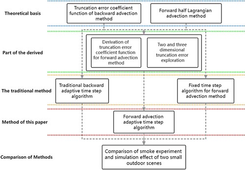
As shown in Figure 1, the algorithm proposed in this study is based on the rule of truncation error coefficient function of backward advection and first-order forward semi-Lagrangian advection methods. The rule of adaptive step size is mastered through truncation error derivation of the forward advection method and two-dimensional and three-dimensional truncation error experiments. In the experimental part, the effectiveness of the proposed method was verified by comparing it with the non-adaptive time-step forward and traditional backward advection adaptive methods.

Figure 1. Methods framework diagram.

2.2. Forward semi-lagrangian advection method

2.2.1 Principles of traditional semi-Lagrangian method and forward methods

The semi-Lagrangian method is one of the most common methods to solve advection problems in Earth science and is widely used in model solving. Outdoor diffusion of harmful aerosols is a fluid process, and the Navier-Stokes (N – S) equation is the most appropriate to describe fluid movement. The solution of the N-S equation is an approximate based on intensive calculation by finite element or finite difference method. In this study, the analysis was based on the finite difference method.

The generalised N-S equation is as follows: (1) $\mathrm{\nabla }\cdot u=0$(1) (2) ${\displaystyle \frac{\mathrm{\partial }u}{\mathrm{\partial }t}=-\left(u\cdot \mathrm{\nabla }\right)u+v{\mathrm{\nabla }}^{2}u-\mathrm{\nabla }p/\rho +f}$(2)

Equations (1(1) $\mathrm{\nabla }\cdot u=0$(1) ) and (2(2) ${\displaystyle \frac{\mathrm{\partial }u}{\mathrm{\partial }t}=-\left(u\cdot \mathrm{\nabla }\right)u+v{\mathrm{\nabla }}^{2}u-\mathrm{\nabla }p/\rho +f}$(2) ) are the mass and momentum conservation equations, respectively. The corresponding terms on the right side of Equation (2(2) ${\displaystyle \frac{\mathrm{\partial }u}{\mathrm{\partial }t}=-\left(u\cdot \mathrm{\nabla }\right)u+v{\mathrm{\nabla }}^{2}u-\mathrm{\nabla }p/\rho +f}$(2) ) from left to right are the advection, diffusion, pressure, and external force terms, which can be solved successively by specific methods. In the above equations, u is the velocity, p is the pressure, ρ is the density, v is the viscosity coefficient, and f is the external force.

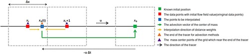
The traditional semi-Lagrangian method is an approximate solution method that relies on feature backward tracking and interpolation. If the velocity field of a study area is equal everywhere, irrespective of time and space, the field generates linear advection. In this case, the transfer of the numerical field can be easily solved and interpolated in reverse.

As shown in Figure 2, the grid centroid at x₀ at time t+Δt was used as the end point, and the corresponding starting position x_d at time t can be found according to the backward tracer, which was obtained from the reverse translation of the average velocity u and the time step Δt. As it is difficult for the position x_d at time t to fall exactly at the centre of mass of the grid, weight interpolation can be performed according to the distance of x_d to the neighbouring centre of mass points x_i and x_i+ 1. Furthermore, the source of flow field interpolation is the centre of mass points xi and x_i+ 1. Finally, the interpolation results are synchronised to x₀ as the flow field value of t+Δt at x₀. As shown in Equation (3(3) $x^{\mathrm{\prime }}{}_j^n=x_j^{n+1}-u\mathrm{\Delta }t$(3) ), the position $x^{\mathrm{\prime }}{}_i^n$ at time n can be obtained by subtracting the displacement from the position at time n + 1, where u is the average velocity from time n to time n + 1 and position $x^{\mathrm{\prime }}{}_i^n$ to position $x_i^{n+1}$; u is constant for linear advection.

Figure 2. Schematic diagram of the traditional semi-Lagrangian advection method.

The absolute linear advection scenario is rare in earth science. The reality is that the velocity field is distributed differently in time and space and, therefore, yields nonlinear advection. For nonlinear advection, the solution method of ordinary numerical field is similar to that of linear advection. However, for the velocity field, it requires an additional special numerical field, and the velocity depends on its own propagation. Therefore, the simple solution method in Figure 2 cannot be used.

To address nonlinear advection, the first step is to calculate the propagation of the velocity field itself, that is, to solve for u. Currently, the intermediate time iteration method is relatively mature: as shown in Equation (4(4) $x_d=x_j^{n+1}-\mathrm{\Delta }tu\left(x\left(t+{\displaystyle \frac{\mathrm{\Delta }t}{2}}\right),t+{\displaystyle \frac{\mathrm{\Delta }t}{2}}\right)$(4) ), $x_d$ is the predicted position at time n; $u\left(x\left(t+{\displaystyle \frac{\mathrm{\Delta }t}{2}}\right),t+{\displaystyle \frac{\mathrm{\Delta }t}{2}}\right)$ is the velocity at the intermediate time and intermediate position. However, they are still difficult to solve. Therefore, Equation (4(4) $x_d=x_j^{n+1}-\mathrm{\Delta }tu\left(x\left(t+{\displaystyle \frac{\mathrm{\Delta }t}{2}}\right),t+{\displaystyle \frac{\mathrm{\Delta }t}{2}}\right)$(4) ) ought to be solved iteratively. Equation (5(5) $x_{d^0}=x_j^{n+1}-\mathrm{\Delta }tu\left(x\left(t+\mathrm{\Delta }t\right),t\right)$(5) ) is set as the initial value of the iteration, and the speed of $x\left(t+\mathrm{\Delta }t\right)$ and $t$is considered as the average speed. Equation (6(6) $x^{\left(k\right)}\left(t+{\displaystyle \frac{\mathrm{\Delta }t}{2}}\right)={\displaystyle \frac{1}{2}\left(x\left(t+\mathrm{\Delta }t\right)+x^{\left(k\right)}\left(t\right)\right)}$(6) ) shows the calculation method of the position at the middle time of the kth iteration. Equation (7(7) $x^{\left(k+1\right)}\left(t\right)=x\left(t+\mathrm{\Delta }t\right)-\mathrm{\Delta }tu\left({\displaystyle \frac{1}{2}\left(x\left(t+\mathrm{\Delta }t\right)+x^{\left(k\right)}\left(t\right)\right),t+{\displaystyle \frac{\mathrm{\Delta }t}{2}}}\right)$(7) ) shows the complete iterative recursion formula, where $x^{\left(k+1\right)}\left(t\right)$ is the tracer endpoint position of the (k + 1)th iteration at time t and $x^{\left(k\right)}\left(t\right)$ is the tracer endpoint position of the (k + 1)th iteration of time t. (3) $x^{\mathrm{\prime }}{}_j^n=x_j^{n+1}-u\mathrm{\Delta }t$(3) (4) $x_d=x_j^{n+1}-\mathrm{\Delta }tu\left(x\left(t+{\displaystyle \frac{\mathrm{\Delta }t}{2}}\right),t+{\displaystyle \frac{\mathrm{\Delta }t}{2}}\right)$(4) (5) $x_{d^0}=x_j^{n+1}-\mathrm{\Delta }tu\left(x\left(t+\mathrm{\Delta }t\right),t\right)$(5) (6) $x^{\left(k\right)}\left(t+{\displaystyle \frac{\mathrm{\Delta }t}{2}}\right)={\displaystyle \frac{1}{2}\left(x\left(t+\mathrm{\Delta }t\right)+x^{\left(k\right)}\left(t\right)\right)}$(6) (7) $x^{\left(k+1\right)}\left(t\right)=x\left(t+\mathrm{\Delta }t\right)-\mathrm{\Delta }tu\left({\displaystyle \frac{1}{2}\left(x\left(t+\mathrm{\Delta }t\right)+x^{\left(k\right)}\left(t\right)\right),t+{\displaystyle \frac{\mathrm{\Delta }t}{2}}}\right)$(7)

The conventional semi-Lagrangian method possesses the disadvantage of non-conservation of mass, and its interpolation method based on the backward tracer may cause the value of the same tracer end neighbourhood to be reused by multiple starting points. Simultaneously, many iterations to approximate the analytical solution incur an additional large computation cost.

In this study, the forward semi-Lagrangian advection method with natural conservation of mass was selected, which has been confirmed by Lentine, Grétarsson, and Fedkiw (2011) in the study of the unconditionally stable semi-Lagrangian method. Moreover, the forward semi-Lagrangian advection method overcomes the disadvantage of the backward tracing method, which relies on an iterative solution, and incorporates the intuitionistic computational process and absolute stability of trajectory with fewer computations (Sun and Yeh 1997). According to Fletcher (2020), geoscience problems require real-time performance in numerical predictions, and on account of an acceptable first-order accuracy of the forward semi-Lagrangian method, in this study, the first-order forward semi-Lagrangian method was selected.

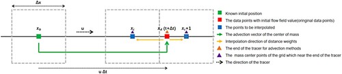
The principle of operation of the first-order forward advection method is to calculate the forward displacement through the velocity and step length. The starting point of the displacement is fixed and the destination position ought to be interpolated. As shown in Figure 3, the grid centroid point at x₀ at time t is the starting point, and the advection end point x_d at time t+Δt is identified according to the forward tracer, which is obtained by the forward translation of the average velocity u and the time step Δt. Similar to the backward method, as it is difficult for x_d at time t+Δt to be obtained exactly at the centre of mass of the grid, the mass of x_d can be assigned to the neighbourhood centre of mass according to the distance between x_d and the neighbourhood centre of mass x_i and x_i+ 1. Furthermore, the sum of the allocated masses ought to be equal to the mass before allocation. Equation (8(8) $x_d=x_0^n+u\mathrm{\Delta }t$(8) ) shows the process of forward advection. Equation (9(9) $x_i=x_d,x_{i+1}=x_d+1$(9) ) shows the calculation method of the neighbourhood grid centroid of the end point $x_d$ of advection. (8) $x_d=x_0^n+u\mathrm{\Delta }t$(8) (9) $x_i=x_d,x_{i+1}=x_d+1$(9)

Figure 3. Schematic diagram of the forward semi-Lagrangian advection method.

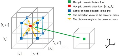
For practical problems, the advection method ought to address the three-dimensional case, as shown in Figure 4. The green particle represents the initial position of the particle cluster (in the centre of the grid), the green arrow represents the forward displacement, the red particle represents the end point of the forward tracer, the blue particle represents the centre of the neighbourhood grid, and the yellow arrow represents the distance weight of the neighbourhood of the centre of mass.

Figure 4. Schematic representation of 3D first-order forward advection interpolation.

2.2.2 Realisation of conservation of mass in forward semi-lagrangian method

Considering Figure 3 as an example, the mass conservation rules of the 1D forward semi-Lagrangian advection method are shown in Equations (10(10) $m_i+m_{i+1}=m_d$(10) ) and (11(11) $m_i=m_d{d}_i=m_d{\displaystyle \frac{\left|x_{i+1}-x_d\right|}{\mathrm{\Delta }x},m_{i+1}=m_d{d}_{i+1}=m_d{\displaystyle \frac{\left|x_i-x_d\right|}{\mathrm{\Delta }x}}}$(11) ): $m_{\mathrm{i}}$ and $m_{\mathrm{i}+1}$ are the mass assigned at grids i and i + 1, and the sum of its values is equal to the original mass $m_{\mathrm{d}}$; in Equation (11(11) $m_i=m_d{d}_i=m_d{\displaystyle \frac{\left|x_{i+1}-x_d\right|}{\mathrm{\Delta }x},m_{i+1}=m_d{d}_{i+1}=m_d{\displaystyle \frac{\left|x_i-x_d\right|}{\mathrm{\Delta }x}}}$(11) ), the value of d is the distance weight, and its effect is that the closer it is to the end point of the forward tracer, the larger the value of the grid centroid point is assigned. The 3D case is similar to the 1D case. Equation (12(12) $m_{i,j,k}+m_{i+1,j,k}+m_{i,j+1,k}+m_{i+1,j+1,k}+m_{i,j+1,k+1}+m_{i+1,j+1,k+1}+m_{i,j,k+1}+m_{i+1,j,k+1}=m_d$(12) ) shows the 3D forward advective mass allocation as shown in Figure 4, which ensures that the sum of the masses allocated by the eight neighbourhood centroid points is equal to the original mass $m_{\mathrm{d}}$. Equation (13(13) $m_{i,j,k}=m_d{d}_i{d}_j{d}_k=m_d{\displaystyle \frac{\left|x_{i+1}-x_d\right|\left|y_{j+1}-y_d\right|\left|z_{k+1}-z_d\right|}{\mathrm{\Delta }{x}^3}}$(13) ) demonstrates the method for obtaining the quality of $m_{i,j,k}$ through linear interpolation. (10) $m_i+m_{i+1}=m_d$(10) (11) $m_i=m_d{d}_i=m_d{\displaystyle \frac{\left|x_{i+1}-x_d\right|}{\mathrm{\Delta }x},m_{i+1}=m_d{d}_{i+1}=m_d{\displaystyle \frac{\left|x_i-x_d\right|}{\mathrm{\Delta }x}}}$(11) (12) $m_{i,j,k}+m_{i+1,j,k}+m_{i,j+1,k}+m_{i+1,j+1,k}+m_{i,j+1,k+1}+m_{i+1,j+1,k+1}+m_{i,j,k+1}+m_{i+1,j,k+1}=m_d$(12) (13) $m_{i,j,k}=m_d{d}_i{d}_j{d}_k=m_d{\displaystyle \frac{\left|x_{i+1}-x_d\right|\left|y_{j+1}-y_d\right|\left|z_{k+1}-z_d\right|}{\mathrm{\Delta }{x}^3}}$(13)

Equation (14(14) $m_{i,j,k}^{nb}=\sum _{n=1}^{nb}{d}_{i_n}{d}_{j_n}{d}_{k_n}{m}_{i_n,j_n,k_n}$(14) ) describes the collection of the interpolation of grid centroid points on the end mass of different sources of forward tracers. Figure 5 shows this process. The blue particle is the centre of mass of the grid $m_{i,j,k}$, the red particle is the end point of the forward tracer within the influence range of the centre of mass $m_{i,j,k}$, and nb is the number of red particles. The influence range of the centroid is larger than that of the grid itself, and the size of the influence range is twice that of the grid. The yellow solid arrow points to the blue centroid point, indicating that the interpolation direction of its distance weight is $m_{i,j,k}$ and its magnitude is the distance weight $d_{i_n}{d}_{j_n}{d}_{k_n}$; the dotted arrow indicates towards the centre of mass of another grid, showing that this component of the mass does not participate in the mass collection of this grid. Equation (15(15) $m_{i,j,k}^{nb+1}{v}_{i,j,k}^{nb+1}=m_{i,j,k}^{nb}{v}_{i,j,k}^{nb}+m_{i_n,j_n,k_n}{v}_{i_n,j_n,k_n}{d}_{i_n}{d}_{j_n}{d}_{k_n}$(15) ) describes the speed transfer process. Based on the mass conservation process of Equations (12)–((14), speed is transferred using momentum conservation. $m_{i,j,k}^{nb}{v}_{i,j,k}^{nb}$ is the total momentum of the grid $m_{i,j,k}$ before the motion, $m_{i_n,j_n,k_n}{v}_{i_n,j_n,k_n}$ is the momentum of the points falling into the influence range of the grid $m_{\mathrm{i},\mathrm{j},\mathrm{k}}$ after the forward tracer, and $d_{i_n}{d}_{j_n}{d}_{k_n}$ is its distance weight. $m_{i,j,k}^{nb+1}{v}_{i,j,k}^{nb+1}$ is the total momentum after momentum fusion, where $m_{\mathrm{i},\mathrm{j},\mathrm{k}}^{\mathrm{n}\mathrm{b}+1}$ is the new mass obtained by Equations (12(12) $m_{i,j,k}+m_{i+1,j,k}+m_{i,j+1,k}+m_{i+1,j+1,k}+m_{i,j+1,k+1}+m_{i+1,j+1,k+1}+m_{i,j,k+1}+m_{i+1,j,k+1}=m_d$(12) )–(14(14) $m_{i,j,k}^{nb}=\sum _{n=1}^{nb}{d}_{i_n}{d}_{j_n}{d}_{k_n}{m}_{i_n,j_n,k_n}$(14) ), and $v_{i,j,k}^{nb+1}$ is the new velocity. (14) $m_{i,j,k}^{nb}=\sum _{n=1}^{nb}{d}_{i_n}{d}_{j_n}{d}_{k_n}{m}_{i_n,j_n,k_n}$(14) (15) $m_{i,j,k}^{nb+1}{v}_{i,j,k}^{nb+1}=m_{i,j,k}^{nb}{v}_{i,j,k}^{nb}+m_{i_n,j_n,k_n}{v}_{i_n,j_n,k_n}{d}_{i_n}{d}_{j_n}{d}_{k_n}$(15) Figures 6 and 7 and Table 1 show the tests for the mass conservation comparison between the methods. Figure 6 shows the aerosol simulation under three conditions in a closed environment: the forward method, the backward method with 5 iterations, and the backward method with 20 iterations. Table 1 is the comparative test of input mass m1 and output mass m2 of the forward semi-Lagrangian method. Thus, m1-m2 is the mass loss, and the smaller its absolute value, the better conservation. At 48 s after the start of the test, the input mass attained 1.96484 g and the mass loss was 7.82E-05 g, which is negligible. Figure 7 shows the visual charts of mass loss under three conditions: the forward method, backward method with 5 iterations, and backward method with 20 iterations. It can be observed that the backward method reduces the mass dissipation by increasing the number of iterations; however, it still has a non-negligible error compared with the forward method.

2.3. Truncation error coefficient function for forward advection method

In the study of Mortezazadeh and Wang (2019), the truncation error coefficient function and the time step setting rule of the backward tracking method were deduced and proved. The forward advection method is similar to the backward method, but the interpolation method has some differences. This study will provide a theoretical basis for adaptive displacement setting by deducing the truncation error coefficient function of the forward advection method.

Figure 5. Mass collection process of grid centroid points in forward advection method.

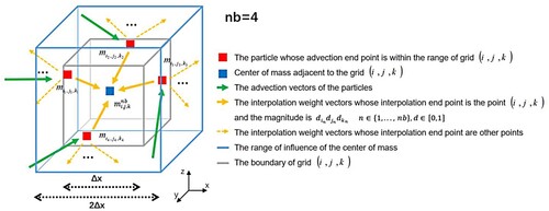
Figure 6. Comparison test of mass conservation between traditional semi-Lagrangian method and forward method under closed condition.

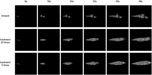
Figure 7. Quality errors of the traditional semi-Lagrangian and forward methods under closed conditions.

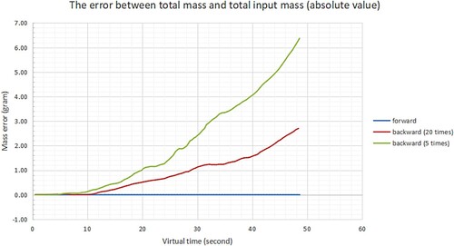
Table 1. Comparison of input quality and output quality of the forward method under closed condition.

t	m1 (mass of input)	m2 (mass of output)	m1-m2
4.5	0.200893	0.200893	−1.49E-08
5.02232	0.222128	0.222128	−4.47E-08
5.5532	0.244161	0.244161	−2.98E-08
6.10403	0.267116	0.267116	5.96E-08
…	…	…	…
47.1115	1.90457	1.90449	7.89E-05
47.6142	1.92467	1.92459	7.53E-05
48.1167	1.94476	1.94469	6.94E-05
48.6189	1.96484	1.96476	7.82E-05

2.3.1. Derivation process of truncation error coefficient function of traditional backward advection method

According to Mortezazadeh and Wang (2019), the Lagrangian interpolation polynomial of one-dimensional backward tracking method for advection field $\phi$ should be expressed as Equation (16(16) ${\phi }_{x_d}\approx \sum _{i=1}^{nb}\left[\left(\prod _{\begin{array}{c}i\le j\le nb\\ j\ne i\end{array}}^{nb}{\displaystyle \frac{\left(x_d-x_j\right)}{\left(x_i-x_j\right)}}\right){\phi }_{x_i}\right]$(16) ), where nb represents neighbourhood interpolation points, $\phi$ is the advection field, the left side of the equation is the value at the starting point $x_d$ of backward tracking, and the right side is the interpolation calculation. The higher the order, the more neighbourhoods are needed and the larger nb. According to Rolle’s theorem, Lagrangian polynomials ought to possess nb number zero points. Thus, the truncation error can be obtained using Equation (17(17) $R_{x_d}=\left|{\displaystyle \frac{1}{nb!}\prod _{j=1}^{nb}\left(x_d-x_j\right){\displaystyle \frac{{\mathrm{\partial }}^{nb}\phi }{\mathrm{\partial }{x}^{nb}}}}\right|$(17) ): (16) ${\phi }_{x_d}\approx \sum _{i=1}^{nb}\left[\left(\prod _{\begin{array}{c}i\le j\le nb\\ j\ne i\end{array}}^{nb}{\displaystyle \frac{\left(x_d-x_j\right)}{\left(x_i-x_j\right)}}\right){\phi }_{x_i}\right]$(16) (17) $R_{x_d}=\left|{\displaystyle \frac{1}{nb!}\prod _{j=1}^{nb}\left(x_d-x_j\right){\displaystyle \frac{{\mathrm{\partial }}^{nb}\phi }{\mathrm{\partial }{x}^{nb}}}}\right|$(17) where $R_{x_d}$ is the truncation error at $x_d$, that is, the difference between the true value of ${\phi }_{x_d}$ and the interpolation on the right side of Equation (16(16) ${\phi }_{x_d}\approx \sum _{i=1}^{nb}\left[\left(\prod _{\begin{array}{c}i\le j\le nb\\ j\ne i\end{array}}^{nb}{\displaystyle \frac{\left(x_d-x_j\right)}{\left(x_i-x_j\right)}}\right){\phi }_{x_i}\right]$(16) ). For the first-order Lagrangian, the interpolation polynomial is given by Equation (18(18) ${\phi }_{x_d}\approx {\displaystyle \frac{\left|x_{i+1}-x_d\right|{\phi }_{x_i}+\left|x_i-x_d\right|{\phi }_{x_{i+1}}}{x_{i+1}-x_i}}$(18) ), and the truncation error is given by Equation (19(19) $R_{x_d}=\left|{\displaystyle \frac{{\mathrm{\partial }}^2{\phi }_d}{2!\mathrm{\partial }{x}^2}\left(x_d-x_i\right)\left(x_d-x_{i+1}\right)}\right|$(19) ). (18) ${\phi }_{x_d}\approx {\displaystyle \frac{\left|x_{i+1}-x_d\right|{\phi }_{x_i}+\left|x_i-x_d\right|{\phi }_{x_{i+1}}}{x_{i+1}-x_i}}$(18) (19) $R_{x_d}=\left|{\displaystyle \frac{{\mathrm{\partial }}^2{\phi }_d}{2!\mathrm{\partial }{x}^2}\left(x_d-x_i\right)\left(x_d-x_{i+1}\right)}\right|$(19)

According to the study of Mortezazadeh and Wang (2019), the truncation error coefficient function is defined as Equation (20(20) $C=\left|\left(x_d-x_i\right)\left(x_d-x_{i+1}\right)\right|$(20) ) from (19): (20) $C=\left|\left(x_d-x_i\right)\left(x_d-x_{i+1}\right)\right|$(20) The truncation error of the second-order one-dimensional Lagrangian interpolation at $x_d$ is a quadratic function of $x_d$, and when $x_d$ passes through points $x_i$ and $x_{i+1}$, the truncation error is zero. $x_i$ and $x_{i+1}$ are two grid centre points, which indicates that the truncation error is zero when the displacement starting point is in the grid centre. As shown in Figure 8, when the starting point of the backward interpolation particle cluster falls at $x_i$ and $x_{i+1}$, its truncation error coefficient is the product of S1 and S2. At this point, Equation (20(20) $C=\left|\left(x_d-x_i\right)\left(x_d-x_{i+1}\right)\right|$(20) ) is a quadratic function of $x_d$, as shown in Figure 9. The truncation error coefficient function of the first-order one-dimensional backward tracking advection is a parabola passing through the zeros of $x_i$ and $x_{i+1}$, and the truncation error reaches the maximum value when $x_d$ is at ${\displaystyle \frac{\mathrm{\Delta }x}{2}}$. Therefore, for the backward method, the truncation error can be minimised by making the starting point of advection close to the centre point of the grid.

Figure 8. Schematic diagram of first-order backward and forward interpolation. Red points are original value points, and blue points are to be interpolated. $x_i$ and $x_{i+1}$ are the centre points of the neighbourhood grid. (a) Backward interpolation. (b) Forward interpolation.

Figure 9. First-order one-dimensional backward tracking truncation error coefficient function image.

2.3.2. Derivation of truncation error coefficient function for forward advection method

As shown in Figures 5 and 8 (b), the forward method means that the particle cluster flows to the new position within the set time according to the flow velocity direction, and then the flow field is allocated to the grid of the neighbourhood according to the weight. At this point, $x_d$ is converted into the original value point, whereas $x_i$ and $x_{i+1}$ are converted into interpolation points, where φ is the mass of the fluid. If the same Lagrange first-order interpolation is used as in 2.3.1, the values of positions $x_i$ and $x_{i+1}$ are divided as shown in Equations (21(21) ${\phi }_i\approx {\displaystyle \frac{\left|x_{i+1}-x_d\right|\phi }{x_{i+1}-x_i}}$(21) ) and (22(22) ${\phi }_{i+1}\approx {\displaystyle \frac{\left|x_i-x_d\right|\phi }{x_{i+1}-x_i}}$(22) ), respectively: (21) ${\phi }_i\approx {\displaystyle \frac{\left|x_{i+1}-x_d\right|\phi }{x_{i+1}-x_i}}$(21) (22) ${\phi }_{i+1}\approx {\displaystyle \frac{\left|x_i-x_d\right|\phi }{x_{i+1}-x_i}}$(22)

This form is similar to Equation (18(18) ${\phi }_{x_d}\approx {\displaystyle \frac{\left|x_{i+1}-x_d\right|{\phi }_{x_i}+\left|x_i-x_d\right|{\phi }_{x_{i+1}}}{x_{i+1}-x_i}}$(18) ), but for the interpolation points on both sides, Equations (21(21) ${\phi }_i\approx {\displaystyle \frac{\left|x_{i+1}-x_d\right|\phi }{x_{i+1}-x_i}}$(21) ) and (22(22) ${\phi }_{i+1}\approx {\displaystyle \frac{\left|x_i-x_d\right|\phi }{x_{i+1}-x_i}}$(22) ) are not standard Lagrangian interpolation forms; thus, the truncation error formula cannot be used. However, it can be converted to a standard format by morphing, as shown in formula (23) and (24):

As shown in Figure 10, two mirror points xd0 and xd1 are added on the basis of Figure 8(b), where the distances from xd0 and xd1 to xd are Δx, and flow field concentration value $\phi$’ of xd0 and xd1 is set to 0. S2’ is equal to S2, and S1’ is equal to S1. Therefore, the interpolation results of the $x_i$ and $x_{i+1}$ positions can be expressed as Equations (23(23) ${\phi }_i\approx {\displaystyle \frac{\left|x_{i+1}-x_d\right|\phi +\left|x_i-x_d\right|{\phi }^{\mathrm{\prime }}}{x_{i+1}-x_i}}$(23) ) and (24(24) ${\phi }_{i+1}\approx {\displaystyle \frac{\left|x_i-x_d\right|\phi +\left|x_{i+1}-x_d\right|{\phi }^{\mathrm{\prime }}}{x_{i+1}-x_i}}$(24) ): (23) ${\phi }_i\approx {\displaystyle \frac{\left|x_{i+1}-x_d\right|\phi +\left|x_i-x_d\right|{\phi }^{\mathrm{\prime }}}{x_{i+1}-x_i}}$(23) (24) ${\phi }_{i+1}\approx {\displaystyle \frac{\left|x_i-x_d\right|\phi +\left|x_{i+1}-x_d\right|{\phi }^{\mathrm{\prime }}}{x_{i+1}-x_i}}$(24)

Figure 10. Schematic diagram of forward interpolation mirror deformation method.

Equation (23(23) ${\phi }_i\approx {\displaystyle \frac{\left|x_{i+1}-x_d\right|\phi +\left|x_i-x_d\right|{\phi }^{\mathrm{\prime }}}{x_{i+1}-x_i}}$(23) ) and (24) can be treated as Lagrange polynomials, and the truncation error coefficient function of the two can be obtained from Equation (25(25) $C_i=C_{i+1}=\left|\left(x_d-x_i\right)\left(x_d-x_{i+1}\right)\right|$(25) ): (25) $C_i=C_{i+1}=\left|\left(x_d-x_i\right)\left(x_d-x_{i+1}\right)\right|$(25) (26) $C_i=\sum _{\begin{array}{c}j=1\\ x_i\le x_{d_j}\le x_{i+1}\end{array}}^n\left|\left(x_{d_j}-x_i\right)\left(x_{d_j}-x_{i+1}\right)\right|+\sum _{\begin{array}{c}k=1\\ x_{i-1}\le x_{d_k}\le x_{i1}\end{array}}^m\left|\left(x_{d_k}-x_{i-1}\right)\left(x_{d_k}-x_i\right)\right|$(26)

For the forward advection interpolation of a single point, the truncation error law of the interpolation points is consistent with that of the backward tracking method. For the point group distributed on the left and right sides of the centre point $x_i$, the truncation error can be expressed as Equation (26(26) $C_i=\sum _{\begin{array}{c}j=1\\ x_i\le x_{d_j}\le x_{i+1}\end{array}}^n\left|\left(x_{d_j}-x_i\right)\left(x_{d_j}-x_{i+1}\right)\right|+\sum _{\begin{array}{c}k=1\\ x_{i-1}\le x_{d_k}\le x_{i1}\end{array}}^m\left|\left(x_{d_k}-x_{i-1}\right)\left(x_{d_k}-x_i\right)\right|$(26) ), where the first term on the right represents the truncation error on the right side of grid $x_i$ and the second term on the right represents the truncation error on the left side of grid $x_i$. Figure 11 shows the image of the advection truncation error coefficient function of the forward method. Among them, the red dot represents the advection end points (original data point) falling into the neighbourhood to the left and right of the centre point $x_i$, the abscissa represents the position of the three advection end points in Figure 11, and the ordinate represents the corresponding truncation error coefficient C.

Figure 11. First-order one-dimensional forward advection truncation error coefficient function.

In Figure 11, $x_{i-1}$ to $x_{i+1}$ is the interpolation interval and the blue and green points are the points to be interpolated; however, the green points are outside this interval. The red points are the original data points which is the point group on the left and right sides of the centre point $x_i$. This interval is divided into left and right intervals, and the red original data points distributed in each interval contribute to the interval endpoints (green and blue) on both sides. In this interval, the contribution of the red points is the interpolation to the blue points, and the interpolation to the green points is the contribution to other intervals. The interpolation data points of the forward method are composed of advection displacement end points from $x_{i-1}$ to $x_{i+1}$. The central blue point to be interpolated cannot be moved, whereas the red points (advection end points) can be obtained by controlling the step size. In Figure 12, two distribution types of displacement endpoints are shown.

Figure 12. Forward method two-advection endpoint distribution types.

According to Equation (21(21) ${\phi }_i\approx {\displaystyle \frac{\left|x_{i+1}-x_d\right|\phi }{x_{i+1}-x_i}}$(21) ) and the conclusion of the backward method, the closer the distribution mode is to the centre of the grid, the smaller the truncation error. Therefore, the distribution pattern in Figure 12 (b) is more ideal than that in Figure 12 (a).

2.4. An adaptive time step algorithm for forward advection method

2.4.1. Multidimensional case of the forward advection method

For the multidimensional case, the truncation error can be regarded as the magnitude of the multidimensional vector, which consists of multiple one-dimensional components. Therefore, we can use the $l_2$ norm to calculate: (27) $|\left|C\right|{|}_2=\sqrt{\sum _{t=1}^n{C}_t^2}$(27)

In Equation (27(27) $|\left|C\right|{|}_2=\sqrt{\sum _{t=1}^n{C}_t^2}$(27) ), t represents dimension, which means the Euclidean distance of multiple one-dimensional components. Unlike the one-dimensional case, this function does not necessarily have a fixed period; thus, its range needs to be determined in advance. The dimension with the largest component value in the multidimensional case can be set as the X direction. Figure 13 shows the characteristics of the X component under different Courant – Friedrichs – Lewy (CFL) values in the two-dimensional case.

Figure 13. Interpolation characteristics of different CFL values of X-axis components.

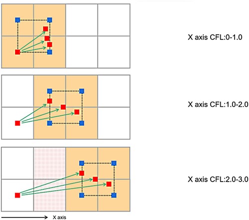
In Figure 13, the gray border is the grid boundary, the red particle is the advection point, and the blue point is the grid centre within the interpolation range. When the CFL value of the X component is between 0 and 2.0, no gap can be obtained between the flow starting point and the interpolation point, whereas when the CFL value is >2.0, a gap is generated (red scatter area). The flow simulation is expected to be ‘continuous’. Therefore, the scope of the study ought to be set such that the 0 < CFL ≤ 2. Figure 14 shows a schematic of flow direction slope.

Figure 14. Slope setting of flow direction.

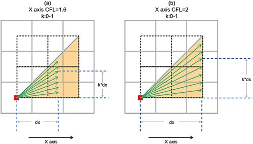
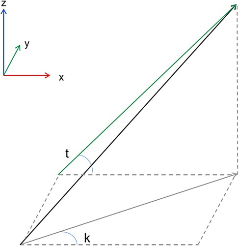
In Figure 14, the slope ranges from 0 to 1. Because of the symmetry, in two dimensions, the difference between the slopes at 0 and 1 covers all angles and k is used to represent the slope of the Y-axis along the X-axis. For the three-dimensional case, t is used to represent the slope of the z-axis on the X-axis, as shown in Figure 15.

Figure 15. Schematic diagram of slope in 3D.

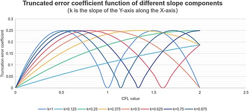
According to the above value conditions, truncation error coefficient functions of different slope components can be obtained within the range of CFL value of 0–2, as shown in Figure 16.

Figure 16. Truncation error coefficient functions of different slope components.

Figure 16 shows that different slopes affect the period of component functions. The truncation error of the two-dimensional function is calculated by the $l_2$ norm, and the image shown in Figure 17 can be obtained. The truncation error of the three-dimensional function was calculated by $l_2$ norm, and four t-slope graphs were obtained, as shown in Figure 18.

Figure 17. Two-dimensional truncation error coefficient function image.

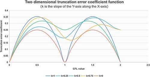
Figure 18. Four three-dimensional truncation error coefficient function images of t-slope.

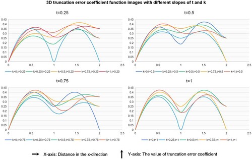
Figures 17 and 18 show that with the principal component direction as the X-axis, the overall increase and decrease of the function is almost unchanged in the two-grid step interval, and the truncation error coefficient function is humped and can reach the minimum value when the principal component is at the centre of the grid.

2.4.2. Forward advection adaptive step size algorithm based on truncation error

The adaptive step size algorithm based on truncation error was used to calculate the global adaptive step size according to the local velocity principal component and truncation error law, and its purpose was to make the end point of more advection points close to the grid centre point. Equations (28) – (31) show the main process of the algorithm: (28) $u=\left(u_s,u_t,u_r\right)$(28) (29) $u_x=Max\left(u_s,u_t,u_r\right)$(29) (30) $\mathrm{\Delta }{t}_l={\displaystyle \frac{C\mathrm{\Delta }h}{u_x}}$(30) (31) $\mathrm{\Delta }{t}_g={\displaystyle \frac{{\sum }_{l=1}^{l_{max}{\sum }_l}{\phi }_l}{{\sum }_{l=1}^{l_{max}\sum }{\phi }_l}}$(31)

Equations (28(28) $u=\left(u_s,u_t,u_r\right)$(28) ) and (29(29) $u_x=Max\left(u_s,u_t,u_r\right)$(29) ) show the process of taking the principal component of local velocity. Equation (30(30) $\mathrm{\Delta }{t}_l={\displaystyle \frac{C\mathrm{\Delta }h}{u_x}}$(30) ) yields the local optimal time step, where C is the Courant number coefficient and the value range is 1 and 2. Equation (31(31) $\mathrm{\Delta }{t}_g={\displaystyle \frac{{\sum }_{l=1}^{l_{max}{\sum }_l}{\phi }_l}{{\sum }_{l=1}^{l_{max}\sum }{\phi }_l}}$(31) ) is the global adaptive step size calculation, where $\phi$ is the concentration field, the global step size of which is equal to the weighted average of the local step size.

2.4.3. Vertical force calculation based on density difference

The wind field is the primary influence on the horizontal movement of aerosol; the density difference causes the vertical movement of air mass, and the primary factor affecting the density is temperature and humidity (Ma et al. 2017). In general, if the research object is not water mist, the solution process is simplified to the solution of temperature difference.

Equation (32(32) $PV=nRT$(32) ) of the thermodynamic equation of gas shows the factors that affect the physical properties of air, where P is the atmospheric pressure, V is the volume, n is the amount of substance, R is the thermodynamic coefficient, and T is the Kelvin temperature. As both V and n are factors affecting density, Equation (32(32) $PV=nRT$(32) ) can be transformed into Equation (36(36) $\rho ={\displaystyle \frac{PM}{RT}}$(36) ): air density is proportional to P and inversely proportional to T. M is the molar mass, which is a constant describing the mass of a mole of material. Equation (33(33) $F_{\mathrm{b}\mathrm{u}\mathrm{o}\mathrm{y}\mathrm{a}\mathrm{n}\mathrm{c}\mathrm{y}}={\rho }_{\mathrm{m}\mathrm{e}\mathrm{d}\mathrm{i}\mathrm{u}\mathrm{m}}Vg$(33) ) is the buoyancy calculation formula in the medium, and Equation (34(34) $F_G=\rho Vg$(34) ) is the fluid gravity formula. The difference is that the ρ in Equation (33(33) $F_{\mathrm{b}\mathrm{u}\mathrm{o}\mathrm{y}\mathrm{a}\mathrm{n}\mathrm{c}\mathrm{y}}={\rho }_{\mathrm{m}\mathrm{e}\mathrm{d}\mathrm{i}\mathrm{u}\mathrm{m}}Vg$(33) ) is the concentration of the solvent, and ρ in Equation (34(34) $F_G=\rho Vg$(34) ) is the concentration of the fluid itself. Therefore, according to Equations (33(33) $F_{\mathrm{b}\mathrm{u}\mathrm{o}\mathrm{y}\mathrm{a}\mathrm{n}\mathrm{c}\mathrm{y}}={\rho }_{\mathrm{m}\mathrm{e}\mathrm{d}\mathrm{i}\mathrm{u}\mathrm{m}}Vg$(33) ) and (34(34) $F_G=\rho Vg$(34) ), the resultant force of the particle cluster can be calculated, namely, F in Equation (35(35) $F_{\mathrm{r}\mathrm{e}\mathrm{s}\mathrm{u}\mathrm{l}\mathrm{t}\mathrm{a}\mathrm{n}\mathrm{t}\mathrm{f}\mathrm{o}\mathrm{r}\mathrm{c}\mathrm{e}}=({\rho }_{medium}-\rho )Vg$(35) ). According to the formula of ρ in Equation (36(36) $\rho ={\displaystyle \frac{PM}{RT}}$(36) ) in combination with Equation (35(35) $F_{\mathrm{r}\mathrm{e}\mathrm{s}\mathrm{u}\mathrm{l}\mathrm{t}\mathrm{a}\mathrm{n}\mathrm{t}\mathrm{f}\mathrm{o}\mathrm{r}\mathrm{c}\mathrm{e}}=({\rho }_{medium}-\rho )Vg$(35) ), the resultant force acceleration a in the vertical direction can be derived, as shown in Equation (37(37) $a_{\mathrm{r}\mathrm{e}\mathrm{s}\mathrm{u}\mathrm{l}\mathrm{t}\mathrm{a}\mathrm{n}\mathrm{t}\mathrm{f}\mathrm{o}\mathrm{r}\mathrm{c}\mathrm{e}}=({\displaystyle \frac{P_0{T}_1}{P_1{T}_0}-1)g}$(37) ). In Equation (37(37) $a_{\mathrm{r}\mathrm{e}\mathrm{s}\mathrm{u}\mathrm{l}\mathrm{t}\mathrm{a}\mathrm{n}\mathrm{t}\mathrm{f}\mathrm{o}\mathrm{r}\mathrm{c}\mathrm{e}}=({\displaystyle \frac{P_0{T}_1}{P_1{T}_0}-1)g}$(37) ), P₀ and T₀ are the air pressure and temperature of the entire environment, and P₁ and T₁ are the air pressure and temperature of the smoke area, respectively. Therefore, a high aerosol temperature or low ambient temperature will accelerate the floating of aerosol particles. Owing to the cooling effect of ambient air, aerosol particles will gradually tend to be distributed at a certain vertical height, until the temperature is consistent with the environment. (32) $PV=nRT$(32) (33) $F_{\mathrm{b}\mathrm{u}\mathrm{o}\mathrm{y}\mathrm{a}\mathrm{n}\mathrm{c}\mathrm{y}}={\rho }_{\mathrm{m}\mathrm{e}\mathrm{d}\mathrm{i}\mathrm{u}\mathrm{m}}Vg$(33) (34) $F_G=\rho Vg$(34) (35) $F_{\mathrm{r}\mathrm{e}\mathrm{s}\mathrm{u}\mathrm{l}\mathrm{t}\mathrm{a}\mathrm{n}\mathrm{t}\mathrm{f}\mathrm{o}\mathrm{r}\mathrm{c}\mathrm{e}}=({\rho }_{medium}-\rho )Vg$(35) (36) $\rho ={\displaystyle \frac{PM}{RT}}$(36) (37) $a_{\mathrm{r}\mathrm{e}\mathrm{s}\mathrm{u}\mathrm{l}\mathrm{t}\mathrm{a}\mathrm{n}\mathrm{t}\mathrm{f}\mathrm{o}\mathrm{r}\mathrm{c}\mathrm{e}}=({\displaystyle \frac{P_0{T}_1}{P_1{T}_0}-1)g}$(37)

2.5. Experimental methods

Small and medium-sized outdoor aerosols are often difficult to simulate in experiments because the surface model simulated at small sizes is often more detailed and the ground objects of three-dimensional digital surfaces affect the simulation effect. However, many application scenarios of aerosol hazards occur at small scales and complex spaces. Therefore, small-scale and full-size model experiments were selected for this experiment (Weng et al. 2014). Two types of digital ground surfaces were selected to construct computing regions under the spatial resolution of 1 m. The simulation effects of the fast algorithm proposed in this study were compared with those of the traditional backward adaptive method and the forward fixed time step method.

The remote sensing test site of Huailai County, Hebei Province, China, and its surrounding areas were selected as the experimental areas. The study area was located in the middle of the Huaiyan Basin at the junction of Hebei Province and Beijing. Within 10 km of the test site, the land surface is rich, including farmland, water, mountains, grasslands, and wetland mudflats. Wind resources are abundant, with wind farms in the west. There are rockeries, houses, vegetation, and other ground objects in the test site. The open terrain near the experimental area is conducive to aerosol dispersion. In this area, tilted photographic models of 500 m × 500 m were obtained (Figure 19).

Figure 19. Tilted photographic model of the experimental area.

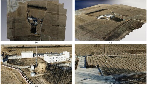
He, Song, and Zhang (2012) used flat and complex terrains for comparative experiments in the study of the influence of surface temperature on wind field simulation. The flat terrain was the open terrain with barrier-free occlusion in the direction of the lower tuyere, whereas the complex terrain comprised relief and was covered by various ground features. The current study used a similar comparison method: in the experimental area, a field was selected as simple terrain and a rockery as a complex terrain contrast experiment. The field was in the direction of the wind outlet of the day and the terrain was flat. The terrain near the rockery was complex, composed of tall soil slope, rock mass, buildings, and vegetation.

2.5.1. Experimental design

The equipment required for the experiment included a mechanical meteorological instrument for measuring temperature, humidity, wind speed, direction, and pressure, the data update frequency of which was every 10 s; a hand-held infrared high temperature thermometer (−40 °C–500 °C); a Dji Jingwei M300 flight platform with a 35 mm lens full frame visible light camera; a high-precision electronic scale; solid smoke cake; and OpenSceneGraph (OSG) development environment (developed by OpenGL technology, which is a set of application programme interfaces based on the C++ platform).

The following measurement information were included: real-time temperature of smoke point, air temperature, ground temperature, digital surface model of the experimental scene, real-time wind speed and direction, mass dissipation of smoke cake, and real-time smoke image.

The experimental process is as follows:

1. A smoke aerosol simulation platform was developed based on adaptive time step algorithm combined with OSG environment.

2. The digital surface model was transformed into a discrete voxel grid for fluid computation.

3. Two types of terrain were selected in the experimental area: simple and complex terrains. Smoke cakes were lit (a cylindrical air hood was used to ensure that the initial direction was constant). A drone was used to obtain real-time images while emitting smoke. The weather sensor recorded the wind speed and direction of the tuyere above the smoke point in real time.

4. An electronic scale was used to weigh the quality loss of smoke cake before and after smoking, which was recorded in the experimental file to analyse the smoke concentration.

5. After smoking, the sensor data were exported to the experimental file according to the time series, and input to the simulation platform for the smoke simulation.

6. The control variable method was used to compare the effect of the adaptive time step with the former and backward methods. The fast simulation, forward fixed time step, and traditional backward adaptive time step methods were used to simulate and evaluate the simulation effect with the experimental image. The time performance of the fast simulation and traditional backward adaptive time step methods was then compared.

2.5.2. Evaluation methodology

The evaluation of the smoke simulation should be based on the comparison of the overlap rate of real smoke images. Combined with the evaluation method of simulated flue gas proposed by Gao and Cheng (2019), the kappa coefficient can be used to evaluate the simulation effect. The above results need to be calculated based on five types of pixels:

1. True positive (TP): aerosol range correctly simulated.

2. False negative (FN): aerosol range not simulated.

3. False positive (FP): aerosol range incorrectly simulated.

4. True negative (TN): the non-aerosol range of correct rejection.

5. Whole area (T): calculates the total area of the area.

Based on the above five ranges, the calculation method of Kappa index is as follows: (38) $\sum =(TP+FP)(TP+FN)+(FN+TN)(FP+TN)$(38) (39) $kappa={\displaystyle \frac{T\left(TP+TN\right)-\mathrm{\Sigma }}{T^2-\mathrm{\Sigma }}}$(39)

There has been a mature criterion for measuring the accuracy of the Kappa coefficient before. Here, the classification and evaluation criteria of the Kappa coefficient proposed by Fleiss, Cohen, and Everitt (1969) were directly borrowed, as shown in Table 2:

Table 2. Evaluation criteria of Kappa index.

Kappa value	Evaluate
0.0–0.20	Extremely low consistency
0.21–0.40	General consistency
0.41–0.60	Medium consistency
0.61–0.80	High degree of consistency
0.81–1.0	Almost identical

3. Results and discussion

3.1. Results

3.1.1 Visualisation comparison

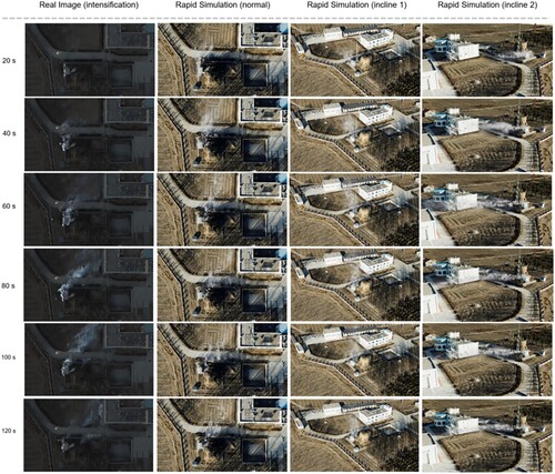
In the experiment of simple terrain, the actual smoke emission time was 102 s. When comparing the results, those obtained every 15 s were selected as the interval for comparison. In the experiment of complex terrain, the actual smoke emission time was 120 s, and the results obtained every 20 s were selected as the interval for comparison. Figure 20 shows from left to right the experimental orthophoto of simple terrain, the orthophoto angle of the simulated results, and the images of two tilted angles of the simulated results. Figure 21 shows the experimental orthophoto of complex terrain, the orthophoto angle of the simulated results, and the images of two tilted angles of the simulated results.

Figure 20. Comparison between full-scale simple terrain experiment and simulation results.

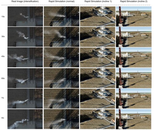
Figure 21. Comparison of full-scale complex terrain experiment and simulation results.

3.2. Evaluation results of the adaptive time step and fixed step methods

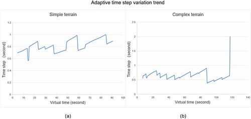
The setting of the fixed time step in the comparison experiment can be determined by the distribution range of the adaptive step. Figure 22 (a) and (b) show the dynamic change of global time step under two types of terrain. The abscissa is the virtual time series and the ordinate is the virtual time step. The virtual time step was generated by the adaptive time step algorithm in Section 2.4.2. javascript:void(0);The virtual time series of simple terrain was 0–90 s and the distribution range of the adaptive time step was 0.5–1 s, whereas the virtual time series of complex terrain was 0–120 s and the distribution range of the adaptive time step was 0.5–2 s.

Figure 22. Adaptive time step change image. (a) simple terrain experiment; (b) complex terrain experiment.

Figure 23 and 24 show the visualisation diagram of the intersection ratio in the forward adaptive step and fixed time step methods under two types of terrain: the simulation area is in red, the experimental smoke area in green, and the overlapping area in yellow. As the step size distribution range of the simple terrain experiment in Figure 22 (a) was 0.5–1 s, fixed time step groups of 0.2 s to 1.5 s were set in Figure 23 for comparison with the adaptive step size. In Figure 22 (b), the step size distribution range of the complex terrain experiment was 0.5–2 s. Therefore, groups ranging from 0.5 s to 2 s were set in Figure 24 for comparison with the adaptive step size. Table 3 shows the data of the average Kappa coefficients classified by the forward adaptive step and the fixed time step methods under two terrains.

Figure 23. Comparison of intersection between simple terrain forward adaptive step size and fixed time step size methods.

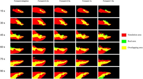
Figure 24. Comparison of the intersection of forward adaptive step size and fixed time step size methods for complex terrain.

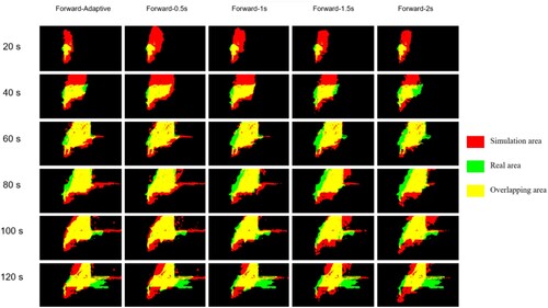
Table 3. Average Kappa values of forward adaptive step size and fixed time step size in simple and complex terrain experiments.

Terrain	Different time step groups
	Forward adaptive	0.2 s	0.5 s	1 s	1.5 s	2 s
Simple terrain	0.47154	0.34269	0.39306	0.46582	0.44044
Complex terrain	0.63513		0.60287	0.61411	0.58263	0.58148

3.3. Evaluation results of forward and backward advection methods

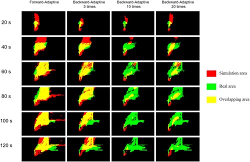
Figure 25 and 26 show the visualisation diagram of the intersection ratio between the forward-adaptive step size method and the backward-adaptive step size method in two types of terrain. Figure 25 and 26 set the forward-adaptive step size group for iteration 5, 10, and 20 times to compare with the forward-adaptive step size. Table 4 shows the data of classification average Kappa coefficients by the forward-adaptive step size method and the backward-adaptive step size method in two terrains. Figure 27 shows the time trend calculation of the forward and backward adaptive step size methods in different groups for the two types of terrain, representing computational complexity.

Figure 25. Comparison of the intersection of forward and backward adaptive step sizes in simple terrain experiment.

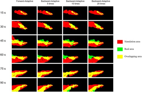
Figure 27. Time trend calculation of forward and backward adaptive steps for two terrain experiments.

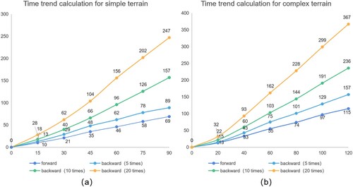
Table 4. Average Kappa values of forward and backward adaptive step sizes in two terrain experiments.

Terrain	Different advection calculation methods
	Forward adaptive	Backward (5 times)	Backward (10 times)	Backward (20 times)
Simple terrain	0.47154	0.46792	0.44044	0.42665
Complex terrain	0.63513	0.62043	0.15709	0.30997

3.4. Visualisation of aerosol three-dimensional motion under different temperature differences using the proposed method

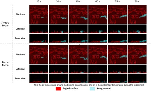
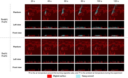
Figure 28 and 29 show the experimental results of the smog-geographic boundary perspective, and the results of the simulation under different temperature differences are shown from three perspectives. The three perspectives show the motion of the simulation method in the vertical direction. T₁ is the measured ambient temperature in the experiment, which is 2 °C. T₀ is the average temperature of the air surrounding the smoke point measured by the thermometer gun. In the experiment, the average temperature surrounding the smoke point was 30 °C. Therefore, the groups of T₀= 30 °C and T₁ = 2 °C simulate the movement of smoke aerosol under the condition of real temperature. The T₀ = 2 °C and T₁ = 2 °C groups simulate the motion of smoke aerosols in the absence of temperature differences. Figure 28 and 29 show the situation under simple and complex terrains, respectively.

Figure 28. Three-dimensional motion visualisation of smoke aerosol in simple terrain under two temperature differences.

3.5. Discussion

3.5.1. Comparative analysis of results of adaptive time step and fixed step methods

In the comparison experiment between the forward adaptive step size and the fixed step size (Figures 23 and 24, and Table 3), we found that the overall accuracy (Kappa) of the adaptive step size method was better than that of the fixed time step.

The Kappa value of the adaptive time step method in the flat ground experiment was 0.47154, which belongs to the evaluation in Table 2: high degree of consistency, and slightly higher than 0.4658 in the 1 s group with fixed step size. As shown in Figure 23, the adaptive method was approximately entirely distributed in the interval of 0.8–1 s. Therefore, the fixed time step of 1 s was closest to the time step required by the optimal truncation error, meaning the results were relatively close. In the rockery experiment, the Kappa value of the adaptive time step method was 0.6351, which constitutes a high degree of consistency with the evaluation in Table 2, and slightly higher than 0.6141 for the 1 s group with fixed step size. The distribution law of adaptive time step is similar to that of flat ground; thus, the fixed time step of 1 s was closest to the time step required by the optimal truncation error.

3.5.2. Comparative analysis of the results of forward and backward advection methods

In the comparison experiment between the forward-adaptive and back-adaptive steps (Figure 25–27, Table 4), we concluded that the overall accuracy (Kappa) of the forward-adaptive step method was better than that of the back-adaptive step method, and the calculation time was far shorter than that of the back-adaptive step method.

Among them, the Kappa value of the forward adaptive step size method in the flat ground experiment was not significantly different from the results of the other groups (the number of iterations was 10 and 20), which were in the range of 0.43–0.47, belonging to moderate consistency (Table 4). In the rockery experiment, the Kappa value of the forward adaptive step size method was much higher than that of the backward method group at 0.6351, indicating a high degree of consistency, whereas the other groups ranged from 0.43–0.47, indicating medium consistency (Table 4). The forward adaptive method had a more significant accuracy advantage than the traditional adaptive method in complex terrain. As shown in Figure 26, more iterations of the backward method resulted in more hysteresis in its flow. This may be related to the numerical dissipation of iterative backward methods in complex neighbourhood problems. The direct flow mechanism of the forward method ensures that it is less affected by the neighbourhood; thus, it is more stable.

Figure 26. Comparison of the intersection of forward and backward adaptive step sizes in complex terrain experiment.

The computing time trends in the two scenarios shown in Figure 27 reflect the inherent advantages of the forward approach. In the case of no GPU acceleration and in a 128*128*20 computing grid, the aerosol-prediction simulation of 90 s could be completed in the ground test at 69 s and that of 120 s could be completed in the rockery test at 115 s. The forward method does not need the characteristic of an iterative solution; thus, it can complete fluid simulation in a virtual time shorter than the real time, which meets the computational requirements of Earth science numerical prediction (Fletcher 2020). The computation time of the backward method linearly increases as the number of iterations increases, and in the experimental environment of this study, the simulation prediction was not completed within the specified time.

3.5.3. Discussion on the three-dimensional motion results of aerosols with different temperature differences

As shown in Figure 28, the simple terrain at the downwind position offers no substantial geographic boundary shielding of smoke aerosol. In the front and left views, the smoke of the experimental group with temperature difference was subject to thermal buoyancy in the vertical direction (calculated according to the method described in Section 2.4.3). The smoke aerosol tended to float up in the initial stage. The aerosols of the control group, which exhibited no temperature difference, were concentrated on the ground, showing a pattern of sticking to the ground. This can be attributed to the control group being affected only by gravity in the vertical direction. From the top view, there was no significant difference between the control group (without temperature difference) and the experimental group (with temperature difference).

The complex terrain at the position of the downwind was covered by large rockery, vegetation, and houses (Figure 29). The diffusion of the control group without temperature difference is not apparent in Figure 29, which is because the lifting effect of buoyancy was lost and its horizontal movement was sufficiently limited by the complex terrain boundary. From the top view, the spatiotemporal patterns of horizontal motion between the groups were significantly different, which illustrates the limiting effect of geographic boundaries on smoke in complex terrain.

Figure 29. Three-dimensional motion visualisation of smoke aerosol in complex terrain under two temperature differences.

The controlled experiments illustrate the necessity of accurate temperature parameters for correct simulation, specifically for complex terrains. In this study, owing to the limitations of experimental equipment, only the temperature at the initial smoke point could be used as the smoke temperature throughout the experiment. If the input of the smoke temperature change curve can be realised, the simulation results of complex terrain will be improved.

4. Conclusions

Aerosols in outdoor scenes are complex geographical phenomena, composed of aerosols themselves, the objective physical environment, and a complex surface. The disadvantages of the traditional advection model make it unsuitable for geo-aerosol simulation.

Based on the N–S fluid model, the forward semi-Lagrange method was used to solve the advancements, and we demonstrated that the adaptive time step based on the first-order forward method to truncate the error coefficient can reduce the theoretical error of the model. Finally, the effectiveness of the method was verified by the full-size outdoor aerosol comparative experiment in complex scenes. In conclusion, the forward adaptive advection method exhibited excellent results towards mass conservation, simulation effect, and computation amount. Moreover, the adaptive step had the advantage of higher accuracy than the fixed step in dealing with variable wind direction. Compared with the traditional backward iteration method, the forward advection method possesses has the advantages of no iteration, less computation, and conservation of mass, and has significant advantages in dealing with complex terrain. The results show that this method is suitable for outdoor aerosol numerical prediction. Because of the limitations of smoke emission sites and environmental protection policies, more experiments at different scales and times were not performed at this stage. Furthermore, the calculation environment of aerosol simulation has not been optimised; therefore, the calculation rate of the experiment is not the final result.

We demonstrate that the adaptive step-size non-iterative advection method performs better than the traditional backward method in complex small-scale scenarios. The next step of this research will focus on the generality of this method to different spatial scales and underlying surface object types. Additionally, the temperature and humidity input models of the algorithm will be improved to better simulate the vertical motion of aerosols. For the future, the proposed advection method is not only suitable for the process simulation of small-scale aerosols but also has a wide application prospect in the geo-advection process of multi-scale and multi-object types.

Disclosure statement

No potential conflict of interest was reported by the author(s).

Additional information

Funding

This research was supported by National Key Research and Development Program of China [grant numbers 2020YFF0400405].

References

- Brzozowska, L. 2014. “Modelling the Propagation of Smoke from a Tanker Fire in a Built-Up Area.” Science of the Total Environment 472: 901–911. doi:10.1016/j.scitotenv.2013.11.130.
- Chen, Z. L. 2012. Research on Aerosol Particle Moving and Heat/Mass Transferring Under Temperature Gradients.” PhD diss., Sichuan University.
- Chu, Y., X. Feng, Q. Zhang, and D. Liang. 2014. “Simulation of Leaking Gas Diffusion in an Urban Using 3D Map Sketch Up.” In 7th International Conference on Intelligent Computation Technology and Automation. 2014: 650–654. doi:10.1109/ICICTA.2014.161.
- Fleiss, J. L., J. Cohen, and B. S. Everitt. 1969. “Large Sample Standard Errors of Kappa and Weighted Kappa.” Psychological Bulletin 72 (5): 323–327. doi:10.1037/h0028106.
- Fletcher, S. J. 2020. “Introduction, Chapter 1.” In Semi-Lagrangian Advection Methods and Their Applications in Geoscience, edited by S. J. Fletcher, 1–5. Elsevier.
- Gao, Y., and P. Cheng. 2019. “Forest Fire Smoke Detection Based on Visual Smoke Root and Diffusion Model.” Fire Technology 55 (5): 1801–1826. doi:10.1007/s10694-019-00831-x.
- Hansen, A. B., J. Brandt, J. H. Christensen, and E. Kaas. 2011. “Semi-Lagrangian Methods in Air Pollution Models.” Geoscientific Model Development 4 (2): 511–541. doi:10.5194/gmd-4-511-2011.
- He, Z. Y., M. X. Song, and X. Zhang. 2012. “Influence of Terrain Surface Temperature on Wind Farm Simulation.” CIESC Journal 63 (Suppl 1): 7–11. doi:10.3969/j.issn.0438-1157.2012.z1.002.
- Lentine, M., J. T. Grétarsson, and R. Fedkiw. 2011. “An Unconditionally Stable Fully Conservative Semi-Lagrangian Method.” Journal of Computational Physics 230 (8): 2857–2879. doi:10.1016/j.jcp.2010.12.036.
- Li, C., and H. Tang. 2022. “Comparison of COVID-19 Infection Risks Through Aerosol Transmission in Supermarkets and Small Shops.” Sustainable Cities and Society 76: 103424. doi:10.1016/j.scs.2021.103424.
- Ma, S. C., J. Chai, K. L. Jiao, L. Ma, S. J. Zhu, and K. Wu. 2017. “Environmental Influence and Countermeasures for High Humidity Flue gas Discharging from Power Plants.” Renewable and Sustainable Energy Reviews 73 (2017): 225–235. doi:10.1016/j.rser.2017.01.143.
- Moreno, T., and W. Gibbons. 2022. “Aerosol Transmission of Human Pathogens: From Miasmata to Modern Viral Pandemics and Their Preservation Potential in the Anthropocene Record.” Geoscience Frontiers 13 (6): 101282. doi:10.1016/j.gsf.2021.101282.
- Mortezazadeh, M., and L. Wang. 2017. “A High-Order Backward Forward Sweep Interpolating Algorithm for Semi-Lagrangian Method.” International Journal for Numerical Methods in Fluids 84 (10): 584–597. doi:10.1002/fld.4362.
- Mortezazadeh, M., and L. Wang. 2019. “An Adaptive Time-Stepping Semi-Lagrangian Method for Incompressible Flows.” Numerical Heat Transfer, Part B: Fundamentals 75 (1): 1–18. doi:10.1080/10407790.2019.1591860.
- Nair, R. D., J. S. Scroggs, and F. H. M. Semazzi. 2003. “A Forward-Trajectory Global Semi-Lagrangian Transport Scheme.” Journal of Computational Physics 190 (1): 275–294. doi:10.1016/S0021-9991(03)00274-2.
- Reisen, F., S. M. Duran, M. Flannigan, C. Elliott, and K. Rideout. 2015. “Wildfire Smoke and Public Health Risk.” International Journal of Wildland Fire 24 (8): 1029–1044. doi:10.1071/WF15034.
- Sheikhnejad, Y., R. Aghamolaei, M. Fallahpour, H. Motamedi, M. Moshfeghi, P. A. Mirzaei, and H. Bordbar. 2022. “Airborne and Aerosol Pathogen Transmission Modeling of Respiratory Events in Buildings: An Overview of Computational Fluid Dynamics.” Sustainable Cities and Society 79: 103704. doi:10.1016/j.scs.2022.103704.
- Staniforth, A., and J. Côté. 1991. “Semi-Lagrangian Integration Schemes for Atmospheric Models—A Review.” Monthly Weather Review 119 (9): 2206–2223. https://doi.org/10.1175/1520-0493(1991)119<2206:SLISFA>2.0.CO;2.
- Sun, W. Y., and K. S. Yeh. 1997. “A General Semi-Lagrangian Advection Scheme Employing Forward Trajectories.” Quarterly Journal of the Royal Meteorological Society 123 (544): 2463–2476. doi:10.1002/qj.49712354415.
- Welander, P. 1955. “Studies on the General Development of Motion in a Two-Dimensional, Ideal Fluid.” Tellus 7 (2): 141–156. doi:10.3402/tellusa.v7i2.8797.
- Weng, M. C., L. X. Yu, F. Liu, and P. V. Nielsen. 2014. “Full-Scale Experiment and CFD Simulation on Smoke Movement and Smoke Control in a Metro Tunnel with One Opening Portal.” Tunnelling and Underground Space Technology 42: 96–104. doi:10.1016/j.tust.2014.02.007.
- Wildhaber, J. H. 2006. “Aerosols: The Environmental Harmful Effect.” Paediatric Respiratory Reviews 7 (Suppl 1): S86–S87. doi:10.1016/j.prrv.2006.04.166.
- Zhao, M., C. Zhou, T. Chan, C. Tu, Y. Liu, and M. Yu. 2022. “Assessment of COVID-19 Aerosol Transmission in a University Campus Food Environment Using a Numerical Method.” Geoscience Frontiers 13 (6): 101353. doi:10.1016/j.gsf.2022.101353