High-resolution spatio-temporal analysis of snowmelt over Antarctic Peninsula ice shelves from 2015 to 2021 using SAR images

ABSTRACT

Ice shelves play an essential role in the dynamics of the Antarctic ice sheet. The surface meltwater is important, as it can irreversibly weaken ice shelves by exerting additional hydrostatic pressure. Therefore, high-resolution snowmelt products are urgently needed to accurately analyze melting patterns of ice shelves and further estimate mass loss. In this study, a new high-resolution (40 m) snowmelt dataset over all of the Antarctic Peninsula ice shelves larger than 100 km${}^2$ was developed based on the modified snowmelt detection framework by using a co-orbit normalization method. The dataset provides detailed snowmelt information on each ice shelf, including the image coverage, melting area and melting ratio every 5 days. The melting patterns of three typical ice shelves (George VI, Wilkins and Larsen C Ice Shelves) and the spatio-temporal melting distribution of the Antarctic Peninsula (AP) were further analyzed. The snowmelt information indicates that both the extent and duration of snowmelt have been increasing in the Antarctic Peninsula from 2015 to 2021, and we found that the snowmelt on the Antarctic Peninsula showed a spatial pattern of significantly intense snowmelt on the western side. We believe this study will provide essential data for ice shelf investigation to support other fields of polar research.

KEYWORDS:

• Surface snowmelt
• ice shelf
• sentinel-1 imagery
• Antarctic Peninsula
• high resolution

1. Introduction

The Antarctic Peninsula (AP), located in the northernmost part of the Antarctic continent, has experienced more dramatic increases in ocean and atmospheric temperatures than the rest of the Antarctic region and is intensely sensitive to climate change (Van Wessem et al. 2016, Liang et al. 2022). The marine margin of the Antarctic Peninsula is greatly influenced by the complex interaction of ice, ocean, atmosphere and inland bed conditions, resulting in the concentration of mass loss (Bell et al. 2018).

As a significant part of this system, the ice shelves around the AP cover an area of 120,000 km${}^2$, playing an essential role in the mass loss and cryospheric processes of the AP. As an important interface between the ice sheet, ocean and atmosphere (Dupont and Alley,2005), ice shelves act to support the inland grounded ice flowing into the ocean (Gudmundsson et al. 2019, Furst et al. 2016). However, several observational studies have shown that ice shelves are retreating and collapsing at an accelerated rate, or even disappearing completely, with an estimated 30,000 km${}^2$ of ice area loss over the past 70 years (Hogg and Gudmundsson,2017, Peck et al. 2010). The extent of seven ice shelves in the AP has been greatly reduced or even completely disappeared (Cook and Vaughan,2010). Therefore, obtaining the dynamic changes of ice shelves in AP is meaningful for accurately estimating the mass loss of Antarctic ice sheets and further understanding ice shelves continuous evolution (Luckman et al. 2014).

Ice sheet melting, as one of the important elements in accurately estimating the surface material loss and surface albedo of the ice sheet, has drawn continued attention from researchers (Liang et al. 2021). Several studies have confirmed that the snowmelt on the surface of the AP is gradually increasing in recent years, contributing 66$\text{\%}$ of the total surface meltwater, while only accounting for 20$\text{\%}$ of the melting extent of the Antarctic ice sheet (Kuipers Munneke et al. 2012, Trusel, Frey, and Das,2012). Meanwhile, as a crucial indicator of ice shelf mass loss, surface melting, which may result in surface lowering and thinning, significantly impacts the stability of ice shelves. During warm summers, meltwater on the surface of ice shelves is stored in the perennial snowpack. Refreezing of surface meltwater releases latent heat into the ice sheet, thereby promoting the accumulation of meltwater on the surface of the ice shelves (Holland et al. 2011, Munneke et al. 2014).

The stability of the ice shelves will be threatened by extensive surface ponding due to changes in stress (Arthur et al. 2020, Dell et al. 2020). If the ice shelf has been substantially damaged by crevasses, natural processes may even initiate meltwater-induced vertical fracturing (Dunmire et al. 2020, Lai et al. 2020). The collapse of the Larsen B ice shelf in 2002 (Domack et al. 2003) is arguably the most famous disintegration event due to its rapid fracturing of only a few weeks likely driven by the drainage of more than 3,000 lakes on its surface caused by the meltwater (Leeson et al. 2020). For that reason, in-depth studies of the melting ice shelves surface snowmelt around the Antarctic Peninsula are critical to accurately estimate of ice shelf mass loss and impact on future climate change (Ingels et al. 2021, Qi et al. 2021).

Microwaves have been widely used to detect meltwater in the Antarctic continent (Guo, Fu, and Liu,2019, Hanna et al. 2013), as they can capture subtle changes in the dielectric constant caused by melting snow and ice. To date, the acquisition of surface snowmelt information mainly relies on microwave radiometer and scatterometer data. Snowmelt detection algorithms using microwave radiometers are mainly divided into the following categories: (1) single-channel/multi-channel brightness temperature snowmelt detection algorithms (Ramage and Isacks,2003, Takala et al. 2008), (2) a snowmelt detection method based on edge detection in time series data (Liu, Wang, and Jezek,2006), and (3) an ice sheet snowmelt detection algorithm using physical models (Ashcraft and Long,2006, Tedesco,2009). Microwave scatterometer data has been used to study snowmelt detection since 2000 as the 4.45 km resolution has obvious advantages over radiometer data with 25 km resolution. The methods most commonly used are classified into the following categories: (1) using threshold backscatter to detect snowmelt (Wismann,2000, Rotschky et al. 2011, Zhao et al. 2014), and (2) model-based algorithms to detect ice sheet surface snowmelt (Ashcraft and Long,2006). Some scholars combined microwave radiometer and scatterometer data for snowmelt detection research (Nghiem et al. 2001, Zheng and Zhou,2020).

Due to the extensive spatial coverage and polar orbits, microwave radiometers and scatterometers can acquire daily snowmelt information over the Arctic and Antarctic. However, the typical spatial resolution of snowmelt products from a spaceborne microwave radiometer and scatterometer ranges from single digits to tens of kilometers, making it challenging to meet the demand for accurate estimation of material loss from the surface of the polar ice sheet (Liang et al. 2021). As a form of active microwave remote sensing, Synthetic Aperture Radar (SAR) is sensitive to the constant dielectric changes caused by ice sheet surface melting. SAR imagery has become a critical data in obtaining high-resolution snowmelt information of the ice sheet with the ability to observe the earth at all times of the day. In particular, with the successive launching of ESA's Sentinel-1 series of satellites, they have provided massive SAR data to monitor polar environments in a short time (Nagler and Rott,1998, Rondeau-Genesse, Trudel, and Leconte,2016).

The time-series and high-resolution information of Antarctic Peninsula ice shelf (APIS) snowmelt not only describes the spatio-temporal melting patterns of ice shelves but also provides fundamental data for further assessing ice shelf mass loss in response to climate change. Considering the abovementioned issues and demand, this study aims to present an ice shelf snowmelt dataset and new contributions in snowmelt research, with the novel points being:

(1)	An automatic ice shelf snowmelt detection framework is proposed and a high-resolution (40 m) snowmelt dataset over the Antarctic Peninsula Ice Shelves is obtained by utilizing the huge amount of Sentinel-1 SAR imagery. The co-orbit normalization method is utilized to overcome the influence caused by the observation geometry, terrain and ice geomorphology.
(2)	The overall melting pattern of the Antarctic Peninsula Ice Shelves from 2015 to 2021 is analyzed based on the high-resolution snowmelt dataset. Meanwhile, the spatio-temporal distribution and pattern of snowmelt in the ice shelf of the Antarctic Peninsula are further investigated.
(3)	The snowmelt dataset provides data support for other polar research, such as monitoring the ice shelves mass balance, investigating ice shelf stability, and understanding the correlation of snowmelt with other climatic factors, especially in the context of global climate change.

2. Study area and data

2.1. The Antarctic Peninsula (AP)

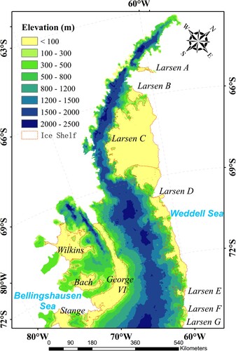
The Antarctic Peninsula is the biggest and northernmost part of the Antarctic. It is located west of the Antarctic, facing South America across the Drake Strait in the north, covering an area from 60${}^{\circ }$W to 75${}^{\circ }$W. The Weddell Sea and the Bellinsgauzen Sea are adjacent to the Antarctic Peninsula in the East and West (Figure 1). There are more than 1,590 glaciers in the Antarctic Peninsula constitute the mountainous terrain, of which the average height is 1,500 m (Johnson, Fahnestock, and Hock,2020).

Figure 1. Location and elevation of ice shelves on the Antarctic Peninsula. The ASTER GDEM is provided by the National Snow and Ice Data Center with a resolution of 100 m. The ice shelves boundary is derived from the MODIS 2003-2004 Mosaic of Antarctica (Scambos et al. 2007), downloaded from the Natural Earth website.

The Antarctic Peninsula is the warmest place in the Antarctic continent, with the most precipitation. Annual precipitation ranges between 500 and 600 mm. The Antarctic Peninsula experiences its highest temperature in January, reaching 1 ${}^{\circ }$C to 2 ${}^{\circ }$C, and the coldest temperature is in June from $-{20}^{\circ }$C to $-{15}^{\circ }$C. Indeed, as Turner et al. (2020) revealed, a positive linear trend in the average annual temperature has been observed at all automatic weather stations located in the Antarctic Peninsula throughout their recording periods. However, the Antarctic Peninsula has experienced much more significant warming than the rest of the Antarctic continent or even other parts of Earth (Bokhorst et al. 2021). Cryospheric processes and ecosystem environments in ice shelf regions are affected by continuing warming temperatures. For instance: (1) the Peninsula saw an increase in ice shelf disintegration rate (Cook and Vaughan,2010, Haug, Kääb, and Skvarca,2010); (2) between 1991–2015, about 52$\text{\%}$ of the glaciers retreated and only 9$\text{\%}$ advanced (Silva et al. 2020); (3) ice loss rate from collapses of ice shelf increased significantly, from 7 ± 13 Gt/yr to 33 ± 16 Gt/yr in the 2010s (Holt et al. 2013).

2.2. Data

2.2.1. Sentinel-1 SAR images

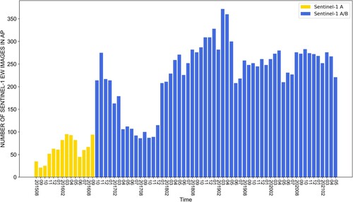
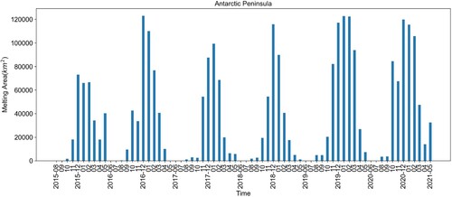
The Sentinel-1 imagery with a swath width of 410 km and a 40 m spatial resolution in EW mode was used in this study. It has an effective revisiting period of six days at the equator, as well as higher frequency image acquisitions in the polar regions due to the polar orbits (Torres et al. 2012, Nagler et al. 2016). The Sentinel-1 satellites provide sufficient data support for the time-series dynamic monitoring of the Antarctic Peninsula. Figure 2 shows that Sentinel-1A captured an average of 60 SAR imagery every month from August 2015 to September 2016. Then from October 2016 after the Sentinel-1B was launched, Sentinel-1A and Sentinel-1B combined were able to obtain an average of approximately 230 scenes per month, with a maximum of nearly 370 scenes, which covers most of the Antarctic Peninsula Ice Shelves area.

Figure 2. Monthly Sentinel-1 image acquisition totals for the Antarctic Peninsula (The orange bar represents the number of image acquisitions before Sentinel-1B was launched, and the blue bar represents the number of image acquisitions after it was launched).

2.2.2. ASTER GDEM of the Antarctic Peninsula

The ASTER GDEM was developed using a method of smoothing snow-covered areas and has a average elevation difference of −4 m from ICESat, as well as a horizontal error of less than 2 pixels. Provided by the National Snow and Ice Data Center (NSIDC), this dataset provides a high-resolution (100 m) DEM of the Antarctic Peninsula (Cook et al. 2012). As in Figure 1, the ice shelves of the AP are concentrated in low-altitude areas near the coastline with a DEM less than 100 m, which are ideal for radar imaging and can effectively alleviate radar shadows and overlay.

2.2.3. Antarctic ice shelf dataset

Obtaining accurate ice shelf boundary information is the key to ensuring precise estimates of ice shelf mass loss. Therefore, the APIS boundary dataset was collected by the United States National Ice Center. The database provides a detailed and accurate description of the extent and boundaries of ice shelves, which were derived from the MODIS Mosaic of Antarctica. In July 2017, the boundaries of Larsen C changed due to the shedding of the A-68 iceberg. To ensure the accuracy of subsequent ice shelf freezing and thawing information, we delineated the boundary line of the Larsen C Ice Shelf after July 2017. In order to ensure the accuracy of the detection results, this study only focuses on ice shelves with an area larger than 100 km${}^2$.

3. Method

3.1. Time-series snowmelt detection framework

The framework of time-series snowmelt detection based on Google Earth Engine (GEE) is proposed in Liang et al. (2021), which mainly has three parts. The first step is data pre-processing. The Sentinel-1 EW data used have been pre-processed for thermal noise removal in GEE. Radiometric correction and topographic correction are also performed using DEM. But before freeze-thaw detection, speckle filtering and black edge removal are still required.

Speckle noise can be removed using widely adopted methods such as Boxcar and refined Lee filter (Lee et al. 2014, Yommy, Liu, and Wu,2015). In this study, Boxcar filter with a window size of $9\times 9$ is used. Black edges refer to invalid edges of Sentinel-1 data in GEE, which may extend as far as tens of kilometers wide and have low and uneven backscattering coefficients. The black edge is close to the backscattering coefficient in ice shelf regions, which may adversely affect the snowmelt detection. Therefore, an entropy value filter is constructed to remove the black edge with lower values.

The snowmelt detection procedure is implemented across the Antarctic after the data pre-processing. As SAR images captured in different orbits have variations in incident angles, resulting in differences in observation geometry and posing great challenges for large-scale snowmelt detection, it is necessary to eliminate these incidental effects. Therefore, co-orbit normalization is utilized in freeze-thaw detection, where the SAR images in austral winter (July and August) are used as a reference to normalize other images in the same orbit. Considering SAR images acquired from the same orbit have the same observation geometry, any differences caused by local incident angles between SAR images can be normalized by subtracting the winter reference images. Extensive experiments have confirmed the success of the co-orbit normalization method in removing the variations in backscattering coefficients caused by SAR observation geometry, terrain fluctuations, and ice geomorphology (Liang et al. 2021). Following this process, a single threshold can be used to distinguish the surface melt in the normalized imagery. In this study, we choose the 5% percentiles of normalized backscattering coefficients ($-2.66$ dB) to detect the surface melt.

The data post-processing includes an image mosaic and mask, accuracy assessment, and map projection. The freeze-thaw imagery are mosaiced and masked by coastline and DEM of the Antarctic to remove the sea ice and high-altitude areas which may cause misidentification. The masked snowmelt maps are projected in the WGS 84 / Antarctic Polar Stereographic Projection to obtain the snowmelt information.

3.2. Time-series ice shelf snowmelt detection

In order to ensure the image coverage of the study area, the snowmelt detection framework merges and normalizes the SAR data of a certain period according to the spatial scale of the data. For continental scales, longer time-series images (one month) are required to obtain snowmelt maps. However, this study focuses on the ice shelf, which can be fully covered by a handful of images, making it possible to increase the product's temporal resolution. We regrouped the melted image collection (an ImageCollection in GEE) acquired through the framework every 5 days. It is notable that for finer spatial scale polar elements the temporal resolution of the product can be further improved.

We used the ReduceRegion method in GEE to directly count the total image coverage area of each ice shelf, the image coverage percentage (the percentage of the image area in relation to the ice shelf vector), and the melting within the image coverage area and unmelted area. We outputted the above parameters as a single file for a specific ice shelf, tremendously reducing the space consumption and time cost. For the polar regions of interest, high-resolution freeze-thaw results can also be downloaded as a file with geo-information.

4. Results

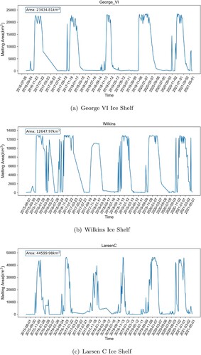
Figure 3 provides time-series snowmelt information for the three typical ice shelves in Antarctic Peninsula (George VI, Wilkins and Larsen C ice shelves, respectively), and Figures A2 and A3 in the Appendix show the time-series snowmelt information of the remaining 11 ice shelves larger than 100 km${}^2$ in the Antarctic Peninsula. In this section, we first analyzed the snowmelt detection results of the aforementioned typical ice shelves, which all have high average melt rates (Kuipers Munneke et al. 2012). Then we qualitatively explored the relationship between surface snowmelt and ice shelf disintegration by studying the calving of the A68 iceberg.

Figure 3. Time-series snowmelt detection information of three typical ice shelves (George VI, Wilkins and Larsen C ice shelf) on the Antarctic Peninsula. (a) George VI Ice Shelf (b) Wilkins Ice Shelf (c) Larsen C Ice Shelf.

4.1. Time-series high-resolution snowmelt detection results of the ice shelves in the Antarctic Peninsula

4.1.1. George VI ice shelf

Figure 3(a) demonstrates the snowmelt information for the George VI Ice Shelf (GVIIS), the second-largest ice shelf on the west coast in the AP. The results indicated that from 2016 to 2018, the snowmelt onset in GVIIS usually from September to October, and intense snowmelt was found in November. The complete melting lasted until February of the following year, with the melting area decreasing significantly in March. Extensive snowmelt occurred in the austral summer of 2019-2020 on the GVIIS, with a significantly earlier onset. The GVIIS melted almost completely in November and lasted until March, with a melting area of 21,942 km${}^2$. For comparison, the George VI ice shelf melted only 8,000 km${}^2$, 7,931 km${}^2$, and 1,178 km${}^2$ from March 2017 to 2019.

Figures 4 and A1 in the Appendix show the high-resolution snowmelt detection result on the GVIIS in 2018/2019 and 2019/2020 austral summer. The surface meltwater was first observed at the northernmost tip of the GVIIS and near the Palmer Land (Figure 4(a)), after which the melting range gradually expanded to the southern GVIIS while being mainly concentrated in the northern GVIIS (Figure 4( b,c)), which is consistent with the fact that the northern GVIIS experiences higher surface summer melt rates (Trusel et al. 2013) and lower accumulation rates. The near-complete melt continued until February (Figure 4(g)), after which the melt gradually diminished but was still concentrated in the northern GVIIS, which can be verified by Figure 4(h).

Figure 4. Freeze-thaw information for the George VI Ice Shelf in 2018/2019. (a) 2018-12-09 (b) 2018-12-14 (c) 2018-12-19 (d) 2018-12-24 (e) 2019-01-18 (f) 2019-02-02 (g) 2019-02-07 (h) 2019-02-12 (i) 2019-02-22.

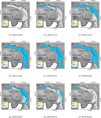
Compared with 2018/2019, GVIIS experienced more intense melting in 2019/2020 austral summer. Figure A1( a,b) in the Appendix showed the time it took for the GVIIS to reach near-complete melt in 2019/2020 was extremely short, only five days, while it took nearly 15 days in 2018/2019. Substantial surface meltwater was found in northern GVIIS, corresponding with periods when daily air temperatures were ≥ 0 ${}^{\circ }$C (Banwell et al. 2021). The near-complete melting of GVIIS continued until March, two months longer than the 2018/2019 melt duration. Figure A1(e–i) in the Appendix clearly shows the freezing process of the southern GVIIS in 2019/2020. The process displays an obvious pattern from southwest to northeast and from low-altitude areas near the coastline more heavily affected by the ocean to high-altitude areas, which will be discussed in detail in Section 5.4.

4.1.2. Wilkins ice shelf

Wilkins Ice Shelf (WIS) is the largest area ice shelf in the West Antarctic Peninsula. Figure 3(b) shows the results obtained from the snowmelt detection framework for the WIS. Melting in the WIS is relatively stable, usually starting in October. Surface snowmelt at the WIS lasts a long time and the ice shelf even partially melted into April and May of the following year (10,552 km${}^2$ in April 2016 and 8,950 km${}^2$ in April 2017). The results also show that the snowmelt of the WIS in 2020 and 2021 was relatively intense, especially in May 2021, with a melting area of 12,305 km${}^2$.

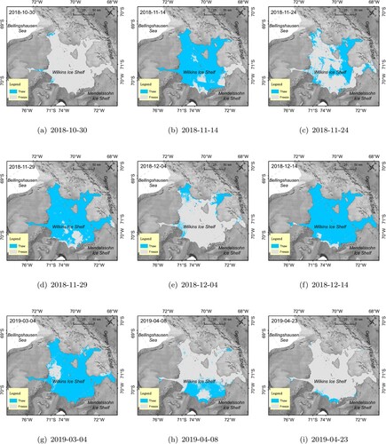
Figure 5 provides information on the snowmelt of the WIS in 2018/2019. During the onset of thawing, substantial meltwater was detected on the surface of the ice shelf. Significantly different from the GVIIS (Shown in Figures 4 and A1), the surface meltwater of the WIS did not accumulate in the early stages of melting. Many regions experienced a thaw-freeze to thaw-refreeze process (Figure 5(c,e)). The near-complete melting continued until mid-March the following year, after which melting gradually subsided and finally melted completely in April 2019. As can be seen from Figure 5(g–i), during the refreezing process, the snowmelt in the western part of the WIS freezes first, possibly affected by warm ocean currents. Conversely, the eastern part of the ice shelf extending to the mainland of the AP melted significantly later than the west.

Figure 5. Freeze-thaw information for the Wilkins Ice Shelf in 2018/2019. (a) 2018-10-30 (b) 2018-11-14 (c) 2018-11-24 (d) 2018-11-29 (e) 2018-12-04 (f) 2018-12-14 (g) 2019-03-04 (h) 2019-04-08 (i) 2019-04-23.

4.1.3. Case study: the impact of snowmelt on Larsen C ice shelf disintegration

Larsen C Ice Shelf (LCIS) is the largest ice shelf on the east coast of the AP and has formed massive subsurface ice (Hubbard et al. 2016). Figure 3(c) presents the melting information of the LCIS. The melting start time varies extremely in different years, but overall the LCIS has a large snow melting area. During the summertime on the Antarctic Peninsula, the melting area of the LCIS exceeds 40,000 km${}^2$. From 2019 to 2021, the melting of the LCIS significantly increased, with a melting area reaching 42,209 km${}^2$ in October.

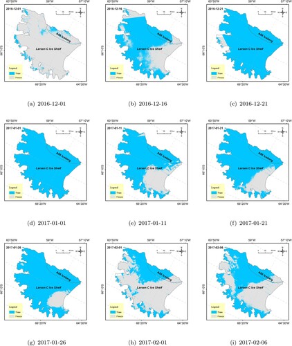
Unusually intense and long-term surface melting is the common precursor to sudden ice shelf collapse (McGrath et al. 2012). In July 2017, the A-68, a 1-trillion-ton iceberg, with an area of 5,800 km${}^2$, broke off from the LCIS. Figure 6 shows the 2016/2017 snowmelt information of the LCIS before the A68 iceberg broke off. During the austral summer, surface snowmelt of the LCIS was significantly intense, which was likely affected by the El Nino phenomenon. And the duration of melt days near the A68 iceberg was significantly higher, as shown in Figure 6(a). Surface meltwater was found on the LCIS when large-scale surface melting has not yet occurred on the LCIS. The melt then gradually spread into the interior of the ice shelf (Figure 6(c–f)), during which the surface of A68 iceberg filled with snowmelt. In February 2017, meltwater was still found on the surface of A68 (Figure 6( h,i)). The high-resolution snowmelt information can show melting patterns of the ice shelf at a finer scale, which allows for qualitative analysis of the correlation between surface snowmelt and ice shelf collapse and disintegration, but an exhaustive explanation for these events still require further research.

Figure 6. Freeze-thaw information for the Larsen C Ice Shelf in 2016/2017 before the A68 Iceberg broke off. (a) 2016-12-01 (b) 2016-12-16 (c) 2016-12-21 (d) 2017-01-01 (e) 2017-01-11 (f) 2017-01-21 (g) 2017-01-26 (h) 2017-02-01 (i) 2017-02-06.

5. Discussion

5.1. Accuracy assessment of ice shelf snowmelt information

Due to the lack of on-site snowmelt data, especially a high-resolution surface melt map, accuracy assessment for melt detection is difficult. In this study, visual interpretation is employed to evaluate the freeze-thaw result accuracy. The visual validation method is based on the decrease in the backscattering coefficient of SAR images caused by meltwater on the surface of ice shelves (Ulaby et al. 1977, Matrosov,2007). It will increase the moisture of the surface, thereby greatly enhancing the dielectric constant and absorbing the electromagnetic waves actively emitted by the SAR sensor, resulting in a decrease in the intensity of the backscattering echo, which is manifested as darkened pixels in the SAR images that can be visually identified as melting regions.

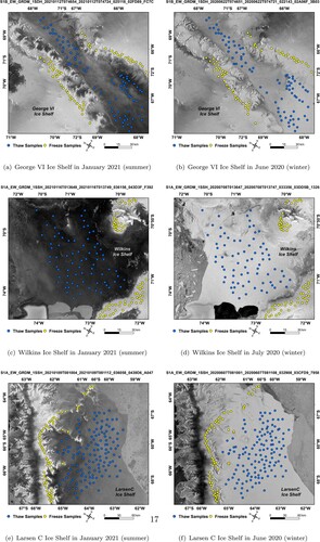
Figure 7 shows the sample images selected for visual interpretation covering the three ice shelves (George VI, Wilkins and Larsen C Ice Shelf, respectively), where the blue samples in the melt areas are thaw samples, while the yellow samples represent the freeze area. The verification points are selected manually by visual interpretation from both freeze and thaw classes in the SAR imagery used in the analysis and their respective winter reference images. When the image pairs of the same orbit are compared and judged, darkened parts of the image were marked as melted and unchanged areas were marked as non-melted. To verify freeze-thaw information, the test samples are distributed as evenly as possible. The SAR imagery in the summer (left column in Figure 7) and winter (right column in Figure 7) clearly shows the melting in the dark region caused by a weak backscattering echo.

Figure 7. Visual interpretation sample selection from Sentinel-1 SAR imagery for ice shelf snowmelt detection. Blue points represent thaw samples, while yellow points represent freeze samples. (a) George VI Ice Shelf in January 2021 (summer) (b) George VI Ice Shelf in June 2020 (winter) (c) Wilkins Ice Shelf in January 2021 (summer) (d) Wilkins Ice Shelf in July 2020 (winter) (e) Larsen C Ice Shelf in January 2021 (summer) (f) Larsen C Ice Shelf in June 2020 (winter).

The accuracy assessment results for the visual interpretation are shown in Table 1, which demonstrates the overall accuracy (OA), Kappa coefficient (Kappa), false positive rate (FPR) and false negative rate (FNR). The OA refers to the proportion of correctly classified samples out of the whole of the samples. FPR represents the proportion of non-melted samples that were detected as melted, while FNR is the proportion of melt samples that were detected as non-melted. The validation results show that the manual visual interpretation has an overall accuracy between 92% to 94% with an average of 93%. The Kappa ranges from 0.88 to 0.92 with an average of 0.90. Based on the accuracy assessment, the manual visual interpretation has a FPR of 5% and a FPR of 6%, respectively. These results confirm the success of the snowmelt detection method.

Table 1. Accuracy assessment for ice shelf snowmelt detection.

Ice Shelf	Overall Accuracy	Kappa	FPR	FPR
George VI	93%	0.91	4%	5%
Wilkins	92%	0.88	4%	6%
Larsen C	94%	0.92	7%	6%
Average	93%	0.90	5%	6%

5.2. Times-series ice shelf snowmelt mapping at a finer resolution

Surface snowmelt in the polar region is one of the sensitive indicators of global climate change (Guo et al. 2020, 2021). Accurate snowmelt assessment helps to understand the melting pattern of the glacier surface, determine its melting state, and analyze the impact on the stability of the ice sheet (Liang et al. 2021). Furthermore, accurate estimates of surface meltwater make it possible to quantitatively assess the role of surface meltwater in ice shelf weakening before disintegration (Kuipers Munneke et al. 2012).

Traditionally, passive microwave imagery has a relatively coarse spatial resolution, with a pixel size of 25 × 25 km${}^2$. However, in most cases, surface meltwater is not homogeneous over a 25 × 25 km${}^2$ range, which results in ‘mixed pixels’ with mixed regions of thaw and freeze. Johnson, Fahnestock, and Hock (2020) compared four passive microwave-based snowmelt detection algorithms with active radar. The results showed that the number of annual melt days varied by up to 30 days at the study site.

Our product has a spatial resolution of 40 m by utilizing Sentinel-1 imagery in the GEE platform. The surface meltwater and spatial patterns of ice shelf melting can be captured more precisely at a finer resolution, especially for smaller ice shelves, which are only a handful of pixels in the radiometer and microwave products. As shown in Figure 4, surface meltwater was found on the GVIIS in the early stage of thawing, and the spatial development pattern of freeze-thaw and thawing was revealed. In Figure A1, it can be seen that the freezing process showed an obvious pattern from southwest to northwest. The snowmelt information can more intuitively reflect the spatial pattern of ice-shelf melting and provide adequate support to explore further and analyze the causes and development of ice shelf melting.

5.3. Surface snowmelt of the Antarctic Peninsula ice shelves from 2015 to 2021

Between 1989 and 2020, the total melting area of the AP was 288,700 km${}^2$ (Trusel et al. 2013), greatly affecting the sea-level and climate change. Figure 8 demonstrates our result of the monthly melt area of the APIS. In 2016, intense melting of AP occurred in October, with a melting area of 42,583 km${}^2$. For comparison, the melting areas in October 2015 and 2017 were 1,632 km${}^2$ and 2,465 km${}^2$, respectively. The melting area peaked at 122,901 km${}^2$ in December 2016, which is in line with the strong El Nio effect and its intense impact on the snowmelt of the Antarctic ice sheets/shelves (Nicolas et al. 2017). The melting intensity of the AP has increased significantly in March in recent years, which is one of the proofs that the AP has experienced a summer retreat. From 2016 to 2019, the average melting area of the AP in March was 28,103 km${}^2$, while the melting areas in 2020 and 2021 were 93,872 km${}^2$ and 47,381 km${}^2$, respectively, which was a significant increase compared to 2016–2019.

Figure 8. The monthly melt area of the Antarctic Peninsula from August 2015 to May 2021. Notably that the data for June and July are missing, as these data were used as reference images to normalize the others.

Our analysis found that in January and February 2020, the melting area reached 122,648 km${}^2$ and 122,350 km${}^2$, respectively, which were 1.36 and 3.01 times in the same period in 2019 (Figure 8), which is in line with the slightly weakened melting trend of the AP in 2017/2018 (Bevan et al. 2018), with a decreasing rate of melt days reaching 20 days every decade. In summary, the time-series high-resolution snowmelt product can be used for accurate monitoring of ice shelf mass loss, analyzing ice shelf melting patterns and correlating melting with large-scale climate processes.

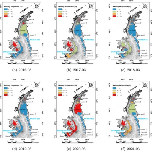
5.4. Spatial melting patterns in the Antarctic Peninsula

Figure 9 shows the melting proportion of ice shelves in March from 2016 to 2021 on the AP. The melting proportion is chosen instead of the melting area as it could more accurately reflect the strength of the melting degree. Figure 9 demonstrates that the melting in the western AP was higher than that in the eastern side, which has been discussed in recent studies finding the melting intensity in the western AP was more intense than that on the east, primarily due to the temperature in the western AP being much higher compared with the same latitudes in the eastern side (Zheng, Zhou, and Wang,2020). Figure 9(b) indicates that five ice shelves in the western AP melted completely in March 2017, and the remaining Stange and GVIIS also had melting ratios of 58.06$\text{\%}$ and 34.4$\text{\%}$, respectively. In contrast, the melting of the ice shelves in the eastern AP did not exceed 30$\text{\%}$ except for the Larsen A Ice Shelf. Nearly the same melting patterns occurred in 2018 and 2019 (Figure 9( c,d)).

Figure 9. Spatial distribution of melting percentage of Antarctic Peninsula ice shelves in March from 2015 to 2021 color-coded from blue (low melting proportion) to red (high melting proportion). The basemap is the Mosaic of cloud-free Moderate Resolution Imaging Spectroradiometer (MODIS) images over the Antarctic Peninsula. (a) 2016-03 (b) 2017-03 (c) 2018-03 (d) 2019-03 (e) 2020-03 (f) 2021-03.

6. Conclusions

This study introduces a high-resolution time-series ice shelf freeze-thaw detection framework for polar regions based on the GEE platform. Benefiting from the co-orbit normalization method, the framework can flexibly adjust the number of images involved in snowmelt detection and the temporal resolution of the product for research regions of different scales by unitizing the huge amount Sentinel-1 SAR imagery.

We obtained the high-resolution (40 m) snowmelt information product of Antarctic Peninsula Ice Shelves with an area greater than 100 km${}^2$ from August 2015 to May 2021. The product can reflect the melting pattern at a finer scale and regularity of a single ice shelf. The snowmelt information suggests that the melting of Antarctic Peninsula Ice Shelves was intense between 2015 to 2021, especially in 2016/2017 and 2020/2021, which may be due to the strong effect of the El Nio phenomenon and extreme weather conditions.

The new snowmelt dataset indicates that the melting of the Antarctic Peninsula shows an apparent spatial-temporal pattern. The average melting area of the APIS reached 106,008 km${}^2$ in December, during which the Larsen C, Wilkins, and George VI Ice Shelves are the major contributors to this snowmelt. In addition, both the duration and extent of the melt have extended in recent years. In particular, the melting area of the Antarctic Peninsula doubled in March and April in the years 2020 and 2021 compared with 2017–2019. Another interesting finding is that the overall melting intensity of the west coast of the Antarctic Peninsula is significantly stronger than that of the east coast.

In summary, the long-term high-precision snowmelt information around the Antarctic Peninsula can effectively fill in the current lack of high-resolution ice shelf surface snowmelt data. The dataset can provide more precise details of ice shelves melting and can accurately observe the spatial distribution pattern of melting, which is difficult to capture with traditional products. We believe our product can be used in a multitude of fields, such as monitoring the ice shelves' mass balance and understanding the correlation of snowmelt with other climatic factors, especially in the context of global climate change. Nevertheless, the characterization methods for polar ice shelf information statistics focus on freeze and thaw, which alone cannot accurately describe the melting intensity of ice sheets. Future studies are still required to pay more attention to the extraction and analysis of quantitative snowmelt indicators.

Acknowledgments

The authors thank Google for providing Google Earth Engine (GEE) platform. The authors also thank Mr Shea Duerler for polishing the language of the paper. The authors highly appreciate Executive Editor-in-Chief Dr Changlin Wang, Chief Managing Editor Dr Zhen Liu, and three anonymous reviewers for their constructive comments and suggestions, which significantly improved the quality of this paper.

Disclosure statement

No potential conflict of interest was reported by the author(s).

Data availability statement

The Sentinel-1 imagery is available at the Google Earth Engine data catalog (https://developers.google.com/earth-engine/datasets). The DEM of Antarctic Peninsula and ice shelf boundary are publicly available at National Snow and Ice Data Center (https://nsidc.org/data/nsidc-0516/versions/1) and British Antarctic Survey website (https://data.bas.ac.uk/).

Additional information

Funding

This work was supported by the Joint Funds of the National Natural Science Foundation of China [grant number U2268217], National Natural Science Foundation of China [grant number 41876226], and Innovative Research Program of the International Research Center of Big Data for Sustainable Development Goals [grant number CBAS2022IRP02].

Appendix

Figure A1. Freeze-thaw information for George VI Ice Shelf in 2019/2020. (a) 2019-11-19 (b) 2019-11-24 (c) 2020-02-22 (d) 2020-03-18(e) 2020-03-23 (f) 2020-04-02 (g) 2020-04-12 (h) 2020-05-02 (i) 2020-05-07.

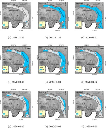
Figure A2. Time-series snowmelt information of ice shelves on the east coast of the Antarctic Peninsula. (a) Larsen A Ice Shelf (b) Larsen B Ice Shelf (c) Larsen D Ice Shelf (d) Larsen E Ice Shelf (e) Larsen F Ice Shelf (f) Larsen G Ice Shelf.

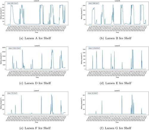
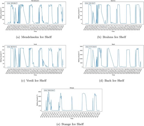
Figure A3. Time-series snowmelt information of ice shelves on the west coast of the Antarctic Peninsula. (a) Mendelssohn Ice Shelf (b) Brahms Ice Shelf (c) Verdi Ice Shelf (d) Bach Ice Shelf (e) Stange Ice Shelf.

References

- Arthur Jennifer F., Chris Stokes, Stewart S. R. Jamieson, J. Rachel Carr, and Amber A. Leeson. 2020. “Recent Understanding of Antarctic Supraglacial Lakes Using Satellite Remote Sensing.” Progress in Physical Geography: Earth and Environment 44 (6): 837–869. doi:10.1177/0309133320916114.
- Ashcraft Ivan S., and David G. Long. 2006. “Comparison of Methods for Melt Detection Over Greenland Using Active and Passive Microwave Measurements.” International Journal of Remote Sensing 27 (12): 2469–2488. doi:10.1080/01431160500534465.
- Banwell Alison F., Rajashree Tri Datta, Rebecca L. Dell, Mahsa Moussavi, Ludovic Brucker, Ghislain Picard, Christopher A. Shuman, and Laura A. Stevens. 2021. “The 32-year Record-High Surface Melt in 2019/2020 on the Northern George VI Ice Shelf, Antarctic Peninsula.” The Cryosphere 15 (2): 909–925. doi:10.5194/tc-15-909-2021.
- Bell Robin E., Alison F. Banwell, Luke D. Trusel, and Jonathan Kingslake. 2018. “Antarctic Surface Hydrology and Impacts on Ice-sheet Mass Balance.” Nature Climate Change 8 (12): 1044–1052. doi:10.1038/s41558-018-0326-3.
- Bevan Suzanne Louise, Adrian John Luckman, Peter Kuipers Munneke, Bryn Hubbard, Bernd Kulessa, and David William Ashmore. 2018. “Decline in Surface Melt Duration on Larsen C Ice Shelf Revealed by the Advanced Scatterometer (ASCAT).” Earth and Space Science 5 (10): 578–591. doi:10.1029/2018EA000421.
- Bokhorst Stef, Peter Convey, Angélica Casanova-Katny, and Rien Aerts. 2021. “Warming Impacts Potential Germination of Non-native Plants on the Antarctic Peninsula.” Communications Biology 4 (1): 1–10. doi:10.1038/s42003-021-01951-3.
- Cook A. J., T. I. Murray, A. Luckman, D. G. Vaughan, and N. E. Barrand. 2012. “Antarctic Peninsula 100 M Digital Elevation Model Derived From ASTER GDEM.” Boulder (CO): National Snow and Ice Data Center. https://doi.org/10.7265/N58K7711.
- Cook Alison J., and David G. Vaughan. 2010. “Overview of Areal Changes of the Ice Shelves on the Antarctic Peninsula Over the Past 50 Years.” The Cryosphere 4 (1): 77–98. doi:10.5194/tc-4-77-2010.
- Dell Rebecca, Neil Arnold, Ian Willis, Alison Banwell, Andrew Williamson, Hamish Pritchard, and Andrew Orr. 2020. “Lateral Meltwater Transfer Across An Antarctic Ice Shelf.” The Cryosphere 14 (7): 2313–2330. doi:10.5194/tc-14-2313-2020.
- Domack Eugene, Amy Leventer, Adam Burnett, Robert Bindschadler, Peter Convey, and Matthew Kirby. 2003. Antarctic Peninsula Climate Variability: Historical and Paleoenvironmental Perspectives. Vol. 79. Washington, DC: American Geophysical Union.
- Dunmire D., J. T. M. Lenaerts, A. F. Banwell, Nander Wever, J. Shragge, Stef Lhermitte, R. Drews, et al. 2020. “Observations of Buried Lake Drainage on the Antarctic Ice Sheet.” Geophysical Research Letters 47 (15): e2020GL087970. doi:10.1029/2020GL087970.
- Dupont T. K., and R. B. Alley. 2005. “Assessment of the Importance of Ice-shelf Buttressing to Ice-sheet Flow.” Geophysical Research Letters 32 (4): 1–4. doi:10.1029/2004GL022024.
- Furst J. J., G. Durand, F. Gillet-Chaulet, L. Tavard, M. Rankl, M. Braun, and O. Gagliardini. 2016. “The Safety Band of Antarctic Ice Shelves.” Nature Climate Change 6: 479–482. doi:10.1038/nclimate2912.
- Gudmundsson G. Hilmar, Fernando S. Paolo, Susheel Adusumilli, and Helen A. Fricker. 2019. “Instantaneous Antarctic Ice Sheet Mass Loss Driven by Thinning Ice Shelves.” Geophysical Research Letters 46 (23): 13903–13909. doi:10.1029/2019GL085027.
- Guo Huadong, Wenxue Fu, and Guang Liu. 2019. Scientific Satellite and Moon-based Earth Observation for Global Change. Singapore: Springer.
- Guo Huadong, Dong Liang, Fang Chen, and Zeeshan Shirazi. 2021. “Innovative Approaches to the Sustainable Development Goals Using Big Earth Data.” Big Earth Data 5 (3): 263–276. doi:10.1080/20964471.2021.1939989.
- Guo Huadong, Stefano Nativi, Dong Liang, Max Craglia, Lizhe Wang, Sven Schade, Christina Corban, G. He, M. Pesaresi, J. Li, and Z. Shirazi. 2020. “Big Earth Data Science: An Information Framework for a Sustainable Planet.” International Journal of Digital Earth 13 (7): 743–767. doi:10.1080/17538947.2020.1743785.
- Hanna Edward, Francisco J. Navarro, Frank Pattyn, Catia M. Domingues, Xavier Fettweis, Erik R. Ivins, Robert J. Nicholls, et al. 2013. “Ice-Sheet Mass Balance and Climate Change.” Nature 498 (7452): 51–59. doi:10.1038/nature12238.
- Haug T., A. Kääb, and P. Skvarca. 2010. “Monitoring Ice Shelf Velocities From Repeat MODIS and Landsat Data – A Method Study on the Larsen C Ice Shelf, Antarctic Peninsula, and 10 Other Ice Shelves Around Antarctica.” The Cryosphere 4 (2): 161–178. doi:10.5194/tc-4-161-2010.
- Hogg Anna E., and G. Hilmar Gudmundsson. 2017. “Impacts of the Larsen-C Ice Shelf Calving Event.” Nature Climate Change 7 (8): 540–542. doi:10.1038/nclimate3359.
- Holland Paul R., Hugh F. J. Corr, Hamish D. Pritchard, David G. Vaughan, Robert J. Arthern, Adrian Jenkins, and Marco Tedesco. 2011. “The Air Content of Larsen Ice Shelf.” Geophysical Research Letters 38 (10): 1–6. doi:10.1029/2011GL047245.
- Holt T. O., Neil F. Glasser, D. J. Quincey, and M. R. Siegfried. 2013. “Speedup and Fracturing of George VI Ice Shelf, Antarctic Peninsula.” The Cryosphere 7 (3): 797–816. doi:10.5194/tc-7-797-2013.
- Hubbard Bryn, Adrian Luckman, David W. Ashmore, Suzanne Bevan, Bernd Kulessa, Peter Kuipers Munneke, Morgane Philippe, et al. 2016. “Massive Subsurface Ice Formed by Refreezing of Ice-shelf Melt Ponds.” Nature Communications 7 (1): 1–6. doi:10.1038/ncomms11897.
- Ingels Jeroen, Richard B. Aronson, Craig R. Smith, Amy Baco, Holly M. Bik, James A. Blake, Angelika Brandt, et al. 2021. “Antarctic Ecosystem Responses Following Ice-shelf Collapse and Iceberg Calving: Science Review and Future Research.” Wiley Interdisciplinary Reviews: Climate Change 12 (1): e682.
- Johnson Andrew, Mark Fahnestock, and Regine Hock. 2020. “Evaluation of Passive Microwave Melt Detection Methods on Antarctic Peninsula Ice Shelves Using Time Series of Sentinel-1 SAR.” Remote Sensing of Environment 250: 112044. doi:10.1016/j.rse.2020.112044.
- Kuipers Munneke P., G. Picard, M. R. Van Den Broeke, J. T. M. Lenaerts, and E. Van Meijgaard. 2012. “Insignificant Change in Antarctic Snowmelt Volume Since 1979.” Geophysical Research Letters 39 (1): 1–5. doi:10.1029/2011GL050207.
- Lai Ching-Yao, Jonathan Kingslake, Martin G. Wearing, Po-Hsuan Cameron Chen, Pierre Gentine, Harold Li, Julian J. Spergel, and J. Melchior van Wessem. 2020. “Vulnerability of Antarctica's Ice Shelves to Meltwater-driven Fracture.” Nature 584 (7822): 574–578. doi:10.1038/s41586-020-2627-8.
- Lee Jong-Sen, Thomas L. Ainsworth, Yanting Wang, and Kun-Shan Chen. 2014. “Polarimetric SAR speckle filtering and the extended sigma filter.” IEEE Transactions on Geoscience and Remote Sensing53 (3): 1150–1160. doi:10.1109/TGRS.2014.2335114.
- Leeson A. A., E. Forster, Amiee Rice, Noel Gourmelen, and J. M. Van Wessem. 2020. “Evolution of Supraglacial Lakes on the Larsen B Ice Shelf in the Decades Before it Collapsed.” Geophysical Research Letters 47 (4): e2019GL085591. doi:10.1029/2019GL085591.
- Liang Dong, Huadong Guo, Qing Cheng, Lu Zhang, and Lingyi Kong. 2022. “Correlation and Interaction Between Temperature and Freeze-thaw in Representative Regions of Antarctica.” International Journal of Digital Earth 15 (1): 2296–2318. doi:10.1080/17538947.2022.2158242.
- Liang Dong, Huadong Guo, Lu Zhang, Yun Cheng, Qi Zhu, and Xuting Liu. 2021. “Time-series Snowmelt Detection Over the Antarctic Using Sentinel-1 SAR Images on Google Earth Engine.” Remote Sensing of Environment 256: 112318. doi:10.1016/j.rse.2021.112318.
- Liang Dong, Huadong Guo, Lu Zhang, Haipeng Li, and Xuezhi Wang. 2021. “Sentinel-1 EW Mode Dataset for Antarctica From 2014–2020 Produced by the CASEarth Cloud Service Platform.” Big Earth Data 6: 385–400. doi:10.1080/20964471.2021.1976706.
- Liang Dong, Huadong Guo, Lu Zhang, Mingwei Wang, Lizhe Wang, Lei Liang, and Zeeshan Shirazi. 2021. “Analyzing Antarctic Ice Sheet Snowmelt with Dynamic Big Earth Data.” International Journal of Digital Earth 14 (1): 88–105. doi:10.1080/17538947.2020.1798522.
- Liu Hongxing, Lei Wang, and Kenneth C. Jezek. 2006. “Automated Delineation of Dry and Melt Snow Zones in Antarctica Using Active and Passive Microwave Observations From Space.” IEEE Transactions on Geoscience and Remote Sensing 44 (8): 2152–2163. doi:10.1109/TGRS.2006.872132.
- Luckman Adrian, Andrew Elvidge, Daniela Jansen, Bernd Kulessa, Peter Kuipers Munneke, John King, and Nicholas E. Barrand. 2014. “Surface Melt and Ponding on Larsen C Ice Shelf and the Impact of Föhn Winds.” Antarctic Science 26 (6): 625–635. doi:10.1017/S0954102014000339.
- Matrosov Sergey Y. 2007. “Modeling Backscatter Properties of Snowfall At Millimeter Wavelengths.” Journal of The Atmospheric Sciences 64 (5): 1727–1736. doi:10.1175/JAS3904.1.
- McGrath Daniel, Konrad Steffen, Harihar Rajaram, Ted Scambos, Waleed Abdalati, and Eric Rignot. 2012. “Basal Crevasses on the Larsen C Ice Shelf, Antarctica: Implications for Meltwater Ponding and Hydrofracture.” Geophysical Research Letters 39 (16): 1–6. doi:10.1029/2012GL052413.
- Munneke Peter Kuipers, Stefan R. M. Ligtenberg, Michiel R. Van Den Broeke, and David G. Vaughan. 2014. “Firn Air Depletion As a Precursor of Antarctic Ice-shelf Collapse.” Journal of Glaciology 60 (220): 205–214. doi:10.3189/2014JoG13J183.
- Nagler Thomas, and Helmut Rott. 1998. “SAR Tools for Snowmelt Modelling in the Project HydAlp.” In IGARSS'98. Sensing and Managing the Environment. 1998 IEEE International Geoscience and Remote Sensing. Symposium Proceedings.(Cat. No. 98CH36174), Vol. 3, 1521–1523. Seattle, WA: IEEE.
- Nagler Thomas, Helmut Rott, Elisabeth Ripper, Gabriele Bippus, and Markus Hetzenecker. 2016. “Advancements for Snowmelt Monitoring by Means of Sentinel-1 SAR.” Remote Sensing 8 (4): 348. doi:10.3390/rs8040348.
- Nghiem S. V., K. Steffen, R. Kwok, and W. Y. Tsai. 2001. “Detection of Snowmelt Regions on the Greenland Ice Sheet Using Diurnal Backscatter Change.” Journal of Glaciology 47 (159): 539–547. doi:10.3189/172756501781831738.
- Nicolas Julien P., Andrew M. Vogelmann, Ryan C. Scott, Aaron B. Wilson, Maria P. Cadeddu, David H. Bromwich, Johannes Verlinde, et al. 2017. “January 2016 Extensive Summer Melt in West Antarctica Favoured by Strong El Niño.” Nature Communications 8 (1): 15799. doi:10.1038/ncomms15799.
- Peck Lloyd S., David K. A. Barnes, Alison J. Cook, Andrew H. Fleming, and Andrew Clarke. 2010. “Negative Feedback in the Cold: Ice Retreat Produces New Carbon Sinks in Antarctica.” Global Change Biology 16 (9): 2614–2623. doi:10.1111/gcb.2010.16.issue-9.
- Qi Mengzhen, Yan Liu, Jiping Liu, Xiao Cheng, Yijing Lin, Qiyang Feng, Qiang Shen, and Zhitong Yu. 2021. “A 15-year Circum-Antarctic Iceberg Calving Dataset Derived From Continuous Satellite Observations.” Earth System Science Data 13 (9): 4583–4601. doi:10.5194/essd-13-4583-2021.
- Ramage Joan M., and Bryan L. Isacks. 2003. “Interannual Variations of Snowmelt and Refreeze Timing on Southeast-Alaskan Icefields, USA.” Journal of Glaciology 49 (164): 102–116. doi:10.3189/172756503781830908.
- Rondeau-Genesse Gabriel, Mélanie Trudel, and Robert Leconte. 2016. “Monitoring Snow Wetness in An Alpine Basin Using Combined C-band SAR and MODIS Data.” Remote Sensing of Environment183: 304–317. doi:10.1016/j.rse.2016.06.003.
- Rotschky Gerit, Thomas Vikhamar Schuler, Jörg Haarpaintner, Jack Kohler, and Elisabeth Isaksson. 2011. “Spatio-temporal Variability of Snowmelt Across Svalbard During the Period 2000–08 Derived From QuikSCAT/SeaWinds Scatterometry.” Polar Research 30 (1): 5963. doi:10.3402/polar.v30i0.5963.
- Scambos Ted A., Terry M. Haran, M. A. Fahnestock, T. H. Painter, and Jennifer Bohlander. 2007. “MODIS-Based Mosaic of Antarctica (MOA) Data Sets: Continent-wide Surface Morphology and Snow Grain Size.” Remote Sensing of Environment 111 (2-3): 242–257. doi:10.1016/j.rse.2006.12.020.
- Silva Aline Barbosa, Jorge Arigony-Neto, Matthias Holger Braun, Jean Marcel Almeida Espinoza, Juliana Costi, and Ricardo Jaña. 2020. “Spatial and Temporal Analysis of Changes in the Glaciers of the Antarctic Peninsula.” Global and Planetary Change 184: 103079. doi:10.1016/j.gloplacha.2019.103079.
- Takala M., J. Pulliainen, M. Huttunen, and Martti Hallikainen. 2008. “Detecting the Onset of Snow-melt Using SSM/I Data and the Self-organizing Map.” International Journal of Remote Sensing 29 (3): 755–766. doi:10.1080/01431160601105934.
- Tedesco M. 2009. “Assessment and Development of Snowmelt Retrieval Algorithms Over Antarctica From K-band Spaceborne Brightness Temperature (1979–2008).” Remote Sensing of Environment 113 (5): 979–997. doi:10.1016/j.rse.2009.01.009.
- Torres Ramon, Paul Snoeij, Dirk Geudtner, David Bibby, Malcolm Davidson, Evert Attema, Pierre Potin, et al. 2012. “GMES Sentinel-1 Mission.” Remote Sensing of Environment 120: 9–24. doi:10.1016/j.rse.2011.05.028.
- Trusel L. D., Karen E. Frey, and Sarah B. Das. 2012. “Antarctic Surface Melting Dynamics: Enhanced Perspectives From Radar Scatterometer Data.” Journal of Geophysical Research: Earth Surface 117 (2): 1–15. doi:10.1029/2011JF002126
- Trusel Luke D., Karen E. Frey, Sarah B. Das, Peter Kuipers Munneke, and Michiel R. Van Den Broeke. 2013. “Satellite-based Estimates of Antarctic Surface Meltwater Fluxes.” Geophysical Research Letters40 (23): 6148–6153. doi:10.1002/2013GL058138.
- Turner John, Gareth J. Marshall, Kyle Clem, Steve Colwell, Tony Phillips, and Hua Lu. 2020. “Antarctic Temperature Variability and Change From Station Data.” International Journal of Climatology 40 (6): 2986–3007. doi:10.1002/joc.v40.6.
- Ulaby Fawwaz T., W. H. Stiles, L. F. Dellwig, and B. C. Hanson. 1977. “Experiments on the Radar Backscatter of Snow.” IEEE Transactions on Geoscience Electronics 15 (4): 185–189. doi:10.1109/TGE.1977.294490.
- Van Wessem J. M., S. R. M. Ligtenberg, C. H. Reijmer, W. J. Van De Berg, M. R. Van Den Broeke, N. E. Barrand, E. R. Thomas, et al. 2016. “The Modelled Surface Mass Balance of the Antarctic Peninsula At 5.5 Km Horizontal Resolution.” The Cryosphere 10 (1): 271–285. doi:10.5194/tc-10-271-2016.
- Wismann Volkmar. 2000. “Monitoring of Seasonal Thawing in Siberia with ERS Scatterometer Data.” IEEE Transactions on Geoscience and Remote Sensing 38 (4): 1804–1809. doi:10.1109/36.851764.
- Yommy Aiyeola Sikiru, Rongke Liu, and Shuang Wu. 2015. “SAR Image Despeckling Using Refined Lee Filter.” In 2015 7th International Conference on Intelligent Human-Machine Systems and Cybernetics, Vol. 2, 260–265. Hangzhou: IEEE.
- Zhao Meng, Joan Ramage, Kathryn Semmens, and Friedrich Obleitner. 2014. “Recent Ice Cap Snowmelt in Russian High Arctic and Anti-correlation with Late Summer Sea Ice Extent.” Environmental Research Letters 9 (4): 045009. doi:10.1088/1748-9326/9/4/045009.
- Zheng Lei, and Chunxia Zhou. 2020. “Comparisons of Snowmelt Detected by Microwave Sensors on the Shackleton Ice Shelf, East Antarctica.” International Journal of Remote Sensing 41 (4): 1338–1348. doi:10.1080/01431161.2019.1666316.
- Zheng Lei, Chunxia Zhou, and Kang Wang. 2020. “Enhanced Winter Snowmelt in the Antarctic Peninsula: Automatic Snowmelt Identification From Radar Scatterometer.” Remote Sensing of Environment 246: 111835. doi:10.1016/j.rse.2020.111835.