A comprehensive method for refining essential SDGs variables for land degradation monitoring based on the DPSIR framework

ABSTRACT

The United Nations adopted 17 Sustainable Development Goals (SDGs) to address societal, economic and environmental sustainability issues. The efficiency of SDGs monitoring could be improved by essential variables (EVs), which can help to better deal with massive data, interdisciplinary knowledge and workloads. However, in practice, effectively combining EVs with SDGs monitoring remains challenging. In this paper, we proposed a refining method of essential SDGs variables (ESDGVs) to land degradation. Firstly, we selected northwest China as our experimental region and extracted a group of variables related to land degradation from SDG indicators based on the DPSIR framework. Next, we identify the essential ones using a combined qualitative and quantitative methods with the criteria of feasibility, spatialization, and relevance which considered the issues of data acquisition, monitoring scale, and closeness to the land degradation. Finally, we analysed the monitoring role of ESDGVs. Results show that, compared to conventional observations, ESDGVs facilitate the monitoring and evaluation of regional SDGs with reduced efforts. And both climate and human activities have a facilitating or inhibiting effect on land degradation processes. In the future, we hope to have more mature data sets and consider adding more SDG indicators for ESDGVs’ refinement.

KEYWORDS:

• Essential SDGs variables
• land degradation
• DPSIR framework
• comprehensive methods
• northwest China

1. Introduction

To solve the contradictions between societies, the economy and the environment, and direct governments’ attention to sustainable development issues, in 2015 the United Nations (UN) adopted 17 Sustainable Development Goals (SDGs) (Chen et al. 2018; Scharlemann et al. 2020; Wang et al. 2021) which help guide and coordinate the participation of governments, agencies, and organizations across countries addressing sustainable development problems and achieving the sustainable use of our common resources (Omisore 2018). The UN then proposed 169 targets and 247 indicators that can express the goals in a more comprehensive way and increase the accuracy and efficiency of their monitoring and evaluation. So far, the SDGs have created an observation system of ‘goals-targets-indicators’ covering many social, economic and environmental problems, with complex meanings and huge structures. Despite significant efforts in related fields, interdisciplinary knowledge, massive data and time-consuming workloads make this work difficult(Plag and Jules-Plag 2020; Lehmann et al. 2020; Guo et al. 2021). For these reasons, some experts introduced the concept of essential variables (EVs), which is extracted from the SDG indicators according to certain rules and provides a set of convenient and operable indicators for monitoring SDGs, based on the assumption that a set of refined variables can facilitate and increase the accuracy of the monitoring process.

The idea of EVs was initially proposed and applied in climate research. In the early stages of climate observations, because of differences in data availability across countries and the decline of the core observation network, there was a need for a set of limited key indicator variables(Houghton et al. 2012). For this reason, the Global Observing System for Climate (Mason et al. 2003) first proposed the concept of Essential Climate Variables (ECVs) and defined them as climate variables that can not only meet the requirements of The United Nations Framework Convention on Climate Change (UNFCCC) but also support global observations. This definition has been constantly improved in subsequent research. Bojinski et al. (2014) defined ECVs more clearly as one or a set of limited physicals, chemical and biological variables that can be used to accurately describe the characteristics of the earth's climate. They also established three principles to be followed in the process of ECVs refinement, namely relevance, feasibility and cost effectiveness. Subsequently, EVs have been applied to biodiversity (Turak et al. 2017)and ocean protection (Miloslavich et al. 2018) research.

Because EVs can be used to dissect complex problems and understand their key information, Reyers et al. (2017) defined essential SDGs variables (ESDGVs) as the minimum variables set representing the change of system characteristics, emphasizing ‘concise and comprehensive’ information to coordinate different activities in the monitoring process of SDGs. The Group on Earth Observation (GEO) defines EVs as a set of relevant physical parameters through which information can be generated from a large number of observations to evaluate specific objectives or policies. Moreover, GEO emphasized that the amount of EVs should be minimized without losing critical information (Nativi et al. 2020). Rosenstock et al. (2017)did not directly mention EVs but pointed out that more extensive data and more frequent monitoring would not necessarily improve target tracking. They believed that the three criteria of consistency, standardization and decision relevance could be followed when designing monitoring schemes. Masó et al. (2020) established several sets of EVs from earth observations, including ECVs and essential biodiversity variables (EBVs), among others. They extracted the SDG indicators that could be monitored with earth observations based on the DPSIR (Driving Force-Pressure-State -Impact-Response) framework and identified the relationship between EVs and SDG indicators, making ESDGVs more than just a concept.

In contrast to those studies that proposed the concept and principles of EVs, some scholars applied EVs to practical monitoring, such as Giuliani et al. (2020) who used a group of Essential Climate Variables in the monitoring of 15.3.1 indicators from the perspective of Earth observation, and Kussul et al. (2020) who identified a set of essential variables from 15.1.1, 15.3.1, 2.4.1 indicators with the help of the water-energy-food model and then assessed these indicators. However, these applications are still relatively few. Due to the great differences in socioeconomic conditions and ecological environments of different countries or regions, the factors affecting the localized extraction and effective monitoring of EVs in SDGs are not clear.

The SDGs cover issues such as poverty, education, climate change and many other social, economic and environmental challenges that we are now dealing with, and land degradation is one of them (Chen et al. 2018). SDG15 indicates that achieving land degradation neutrality is of great significance to biodiversity and the sustainability of terrestrial ecosystems (Tóth et al. 2018). As a great obstacles to the progress of human society, land degradation is considered by international bodies such as the United Nations Convention to Combat Desertification (UNCCD), the Convention on Biological Diversity, and the United Nations Framework Convention on Climate Change as an important challenge on the path to sustainable development (Tucker and Pinzon 2018). The SDG Indicators Metadata repository published by the UN (2022) uses land cover, land productivity, carbon stocks, and the principle of ‘one out, all out’ to measure land degradation. UNCCD has released a Good Practice Guidance report for monitoring SDG 15.3.1 that provides a series of indices by land productivity, land cover, and soil carbon stocks, and shows their formulas and available data sources (Sims et al. 2021). These efforts can help early achievement of land degradation neutrality in a country or region. For example, Germany has included soil quality and land degradation indicators in the National Sustainable Development Strategy in order to achieve SDGs more quickly (Wunder and Bodle 2019). The significance of land degradation research is not only to improve the ecological environment (Sayl et al. 2021). Research shows that there is a vicious cycle between land degradation and poverty (Jiang et al. 2022). For example, the decline of soil fertility and overuse of pesticides can lead to poor harvests, which leads to the decline of local residents’ income, and poverty exacerbates plundering of land resources. In addition to the economy, land degradation is also related to the stability of human societies. The loss of cultivated land and serious desertification are constantly encroaching on human settlements, which directly or indirectly affect human well-being(Sena and Ebi 2021; Senanayake et al. 2022; Masoudi, Vahedi, and Cerdà 2021). Therefore, monitoring SDGs related to land degradation is important not only for environmental protection, but also for social and economic stability (Lal et al. 2021). Understanding the causes and consequences of land degradation can help us capture the key factors and evolution process of this phenomenon and extract all EVs related to land degradation from SDGs on this basis. For this reason, the DPSIR framework is introduced. This framework consists of five components: ‘Drivers-Pressures-Status-Impacts -Response’, allowing for the integration of knowledge from the social, economic and environmental fields and playing a significant role in monitoring sustainable development (Chandrakumar and McLaren 2018; Pellens et al. 2021; Liu et al. 2020). In addition, the DPSIR framework has a certain causal logic, considering what the existing environmental problems are and the root causes and impacts of environmental problems, which helps to explore the evolutionary pattern of land degradation (Liu, Liang, and Hashimoto 2020).

In summary, to address the problems caused by the large monitoring system and the complex meaning of SDGs, this paper introduces the concept of EVs and proposes a combined qualitative and quantitative method for the refinement of ESDGVs. For the first time, we have refined a set of ESDGVs from SDGs indicators that are applicable to Northwest China and related to land degradation with the help of DPSIR framework. This effort will result in a more concise and clearer monitoring of SDGs. In addition, our work analyzes the trends and patterns of land degradation in Northwest China from the perspectives of Driving force, Pressure, State, and Response, which can also help alleviate the severe land degradation problems in Northwest China.

2. Study area and data sources

2.1 Study area

Four provinces in northwest China which are dominated by plateaus, basins and mountains were selected as study areas: Inner Mongolia Autonomous Region, Xinjiang Uygur Autonomous Region, Ningxia Hui Autonomous Region and Gansu Province. They are located between 30°∼ 55°N latitude, 73° ∼ 127°E longitude. The total area is about 3.34 million km². Most of the region has a dry temperate continental climate (Liu, Liang, and Hashimoto 2020b). Arid and semi-arid regions, where evaporation far outweighs precipitation, account for a large proportion of the study area. Wind erosion, poor drainage and intensified evapotranspiration have led to a spread of Gobi and other deserts (Zheng and Yin 2010), as shown in Figure 1, and secondary soil salinization. Northwest China also has a well-developed animal husbandry industry, with two of China's four largest pastoral areas – Inner Mongolia and Xinjiang pasturelands. Overgrazing leads to bare land, reducing grassland biodiversity and soil organic matter, increasing soil vulnerability to desertification and resulting in grassland degradation (Riva et al. 2017). The harsh geography of the northwest makes us realize that social and economic development should go hand in hand with environmental protection. Although some policies have been put forward to improve the environment, studies show that northwest China is still a region with severe desertification and remains a hotspot in land degradation research (Zhang et al. 2021; Wang et al. 2020).

Figure 1. Location and climate of the study area and sampling regions.

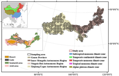
To reflect the state of sustainable development at the regional level, we used regular grids instead of administrative cells as the research units. In our study, we selected 164 sampling regions (100 km × 100 km regular grids) across four provinces (Figure 1). These grids were randomly distributed throughout the research area and covered various terrain and climate types to adequately reflect the environmental and social conditions.

2.2 Data sources

The data used in this experiment mainly included land use, Normalized Difference Vegetation Index (NDVI), Net Primary Productivity (NPP), demographic and meteorological data (Table 1).

Table 1. Data sources used in this study. CNLUCC: China's National Land Use and Cover Change data set; UICUNA: Unconstrained Individual Countries 2000–2020 UN Adjusted data set; SIDAP/MT: the Spatial Interpolation Dataset of Annual Precipitation in China Since 1980 and Spatial Interpolation Dataset of Annual Mean Temperature in China Since 1980.

Dataset	Resolution	Years	Source	Projection	URL
CNLUCC	30m	2000,2005, 2010,2015	Resource and environment science and data center	Krasovsky_1940_Albers	https://www.resdc.cn/Default.aspx
MOD13A3	1000m	2000,2005, 2010,2015	LAADS DAAC	Sinusoidal	https://ladsweb.modaps.eosdis.nasa.gov/search/
MOD17A3HGF	500m	2000,2005, 2010,2015	LAADS DAAC	Sinusoidal	https://ladsweb.modaps.eosdis.nasa.gov/search/order/1/MOD17A3HGF–6
UICUNA	1000m	2000,2005, 2010,2015	WorldPop	WGS84	https://www.worldpop.org/geodata/listing?id = 75
SIDAP/MT	1000m	2000,2005, 2010,2015	Resource and environment science and data center	Clarke_1866_Albers	https://www.resdc.cn/Default.aspx

Land use and land cover change (LUCC) data came from China's National Land Use and Cover Change (CNLUCC), which contains multiple periods of remote sensing monitoring data of LUCC in China (Xu et al. 2018). This data set was visually interpreted by The Chinese Academy of Sciences with Landsat data as the main information source, combined with the National Resources and Environment database. The CNLUCC has better spatial and temporal resolution and higher accuracy than other LUCC products. It adopts a three-level classification system and we used 1st and 2nd level data.

The datasets of NDVI and NPP were from MOD13A3 (Didan) and MOD17A3HGF. The MOD13A3 data set was provided every month with 1-km spatial resolution. The accuracy of this data has been validated after extensive ground validation work. The unit value of MOD17A3HGF data is kg C/m/year. This data set has been available since 2001.

Demographic data were obtained from WorldPop (Lloyd et al. 2019), which provides gridded data. We choose the Unconstrained Individual Countries 2000–2020 UN Adjusted data set which was aggregated to 1-km resolution and where each pixel represents the total number of people in a unit. This product has been adjusted according to the 2019 Revision of World Population Prospects and the mapping approach was a Random Forest-based dasymetric redistribution.

Temperature and precipitation data were from the Spatial Interpolation Dataset of Annual Precipitation in China Since 1980 and Spatial Interpolation Dataset of Annual Mean Temperature in China Since 1980 (SIDAP/MT). The data sets were generated based on daily observations from more than 2,400 meteorological stations across the China with the ANUSPLIN interpolation software (Hutchinson 1998).

3. Methodology

3.1 DPSIR framework

The DPSIR framework was originally proposed by the European Environment Agency to address environmental problems (Lu et al. 2015; Masó et al. 2020). It assumes that the social, economic and environmental systems components are interdependent. The framework consists of five parts, including Driving Force, Pressure, State, Impact and Response. A Driving Force, such as population, economic and societal behaviors produce stressful activities. Pressure is a way of representing how a Driving Force influences a change in State. State is a phenomenon that reflects the existence of a problem. Impact is a change in human well-being resulting from a change in state. The change is generally considered to be negative, but there are also cases of positive effects. Response is an action or strategy designed to reduce the negative impacts (Bradley and Yee 2015). These five parts explore the source of the problem, its adverse effects, and ways to improve it. The framework has been widely used in fields such as biodiversity research, marine ecosystem services, and environmental conservation.

One of the advantages of the DPSIR framework is that it takes human activities into account, especially as a Driving Force. Human activities are the root cause of many environmental problems, such as deforestation; migrations leading to urban sprawl; overgrazing leading to grassland degradation. The SDGs or other sustainable developmental issues can be better addressed by considering the human impact on the surrounding environment. Another advantage of the DPSIR framework is the causality involved (Liu et al. 2020). That is, Driving Forces and Pressure are direct or indirect causes leading to State; State is the main cause of the Impact; Impact is the driver of a Response; and the result of Response is a change in Driving forces, Pressure, State and Impact. This logical relationship is of great significance to the study of land degradation. In this experiment, the calculation of the correlation between variables depended on the causal logic in the framework.

The DPSIR framework in this paper (Figure 2) differs to some extent from the classic framework and is defined as follows.

Figure 2. DPSIR framework of land degradation.

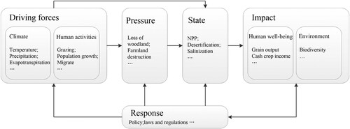
Driving Force is the factor that causes land degradation directly or through pressure; it mainly includes climate and human activities (e.g. population growth, spatial differentiation of temperature and precipitation, and discharge of pollutants).

Pressure is the result of a Driving Force. It leads to the State directly and generally is represented by an environmental variable. For example, when deforestation causes a decrease in forest cover, the bare land worsens erosion which can exacerbate land degradation. In this case, forest cover is one of the Pressure variables.

State is a manifestation of land degradation, such as land productivity or soil salinization. This manifestation can directly reflect the degree and direction of land degradation and have some impacts on human life or environment.

Impact indicates the negative or positive effects of land degradation, the result of State. Most of the Impacts are adverse and threaten human well-being.

Response is a strategy to deal with land degradation. It can slow the rate of land degradation and have a feedback effect on Driving Force, Pressure, State and Impact.

3.2 Technology frame

In the process of refining EVs, most scholars rely on their expert knowledge, which is subjective and qualitative. However, these EVs may no longer be applicable once a study area or study scale changes. EVs should be a concise set of variables without useless information and should reflect the conditions of a study area. The factors impeding sustainable development and land degradation vary from place to place due to climatic, social and cultural differences(Zakerinejad and Masoudi 2019). We should take into account the errors that these differences bring to the monitoring process and refine a set of EVs that can objectively reflect the true local situation. Therefore, this paper proposed a combined quantitative and qualitative approach to specify our process of refining ESDGVs on the uniform grid scale in a normalized way. The qualitative process involves first filtering of variables based on a priori knowledge in terms of operational feasibility and spatialization difficulty. The quantitative process involves adding local observational data, calculating variables and correlations between variables, and discarding variables that have no relationship with land degradation and sustainable development to carry out a second filtering. We normalize the results of qualitative and definite screening with numbers within [0, 1]. The refinement approach incorporates both empirical knowledge and data calculations that objectively represent the state of land degradation and the sustainable development of a region.

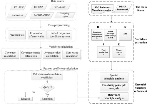
In the flowchart of our experiment (Figure 3), the overall technological framework can be summarized into two parts: the extraction of variables and the refinement of ESDGVs. The first part shows the process of extracting variables from indicators and the second part shows the refinement process of those variables. Detailed steps are as follows.

Figure 3. Flowchart of the refinement process for land degradation related ESDGVs. ** indicates a significance level of 0.01.

3.2.1 Extraction of variables

We analyzed each indicator with the help of the SDG Indicators Metadata Repositoryand Good Practice Guidance, dissecting the relevant indicators to extract variables from them, guided by the DPSIR framework. The SDG Indicators Metadata Repository is constantly updated, providing information on the definition, data sources and rationale. At the time of this writing, it represents the most comprehensive literature explaining SDGs. To ensure that critical information was included, we also refer to the Good Practice Guidance published by UNCCD, which contains numerous indices related to land degradation and SDG 15.3.1. We took them as our main source for extracting variables from indicators with other literature as supplement and extracted the variables related to land degradation from the SDG indicators and grouped them according to the categories of the DPSIR framework. The categorization of the variables and their relationship to the indicators are shown in Table 2.

Table 2. Variables extracted from SDG indicators.

Driving Forces variables	Press variables	State variables
Population distribution (PD) (1, 1)	Cultivated land cover rate (CLCR) (1, 1)	NPP value (NPP) (1, 1)
Population change (PC) (1, 1)	cultivated land cover change (CLCC) (1, 1)	NPP change (NPPC) (1, 1)
Annual precipitation (AP) (1, 1)	Inland water cover rate (IWCR) (1, 1)	Salinized land Cover rate (SLCR) (1, 1)
Annual average temperature (AAT) (1, 1)	Inland water cover change (IWCC) (1, 1)	Salinized land Cover change (SLCC) (1, 1)
	The area of the land occupied by the city/urban area (ALOU) (1, 1)
	Forest cover rate (FCR) (1, 1)
	Forest cover change (FCC) (1, 1)
	NDVI value (NDVI) (1, 1)
	Wetland cover change (WLCC) (1, 1)
	Soil organic carbon (SOC) (0, 1)
Impact variables	Response variables
Soil biodiversity (SO)(0, 1)	Nature reserves cover rate (NRCR) (1, 1)
Output value of grain per unit (OVG)(1, 0)

Note: ‘(0, 1)’ indicates that the data required to calculate the variables are difficult to obtain, i.e. low feasibility; ‘(1, 0)’ indicates that the variables are difficult to spatialize; ‘(1, 1)’ indicates a high degree of feasibility and spatialization.

3.2.2 Refinement of ESDGVs

3.2.2.1 Development of criteria and qualitative screening of variables

Reyers et al. (2017) proposed four criteria to identify essential ESDGVs, namely capturing the system’s essence, linking to system transformations, capturing key areas requiring coordination, and indispensability. GEO identified a set of EVs for SDGs monitoring through the criteria of relevance, feasibility, and Cost-effectiveness (Masó et al. 2020), consistent with ECVs (Bojinski et al. 2014). The criteria of linking to system transformations and capturing key areas requiring coordination are more focused on describing the role of ESDGVs in facilitating cross-domain collaboration. Capturing the system’s essence and indispensability emphasize that the ESDGVs can express the processes, key features, and interactions of the system and it should be indispensable for SDGs monitoring. In other words, the ESDGVs should be most closely relevant to the monitoring objective and its change process, which is consistent with the GEO’s study. Therefore, as a common criterion, relevance is first chosen. Furthermore, the enforceability of a plan is important for the implementation of the monitoring process. Data acquisition, workload, and cost should all be taken into account and are collectively referred to as feasibility in this paper. We added more considerations based on above studies. In order to better monitor land degradation in small-scale areas, we conducted experiments on a grid scale. Therefore, we also consider whether the values of variables can be decomposed on a regular grid, which is the ‘spatialization’ principle.

We finally refined the ESDGVs based on these criteria. Feasibility refers to the ability of data acquisition means such as earth observation technology and maturity of data processing. Spatial refers to the possibility of monitoring EVs on a regional scale rather than administration cells, which is very important for multi-spatial SDGs monitoring. Relevance refers to whether the EVs are relevant with land degradation, both as driving factors or influenced factors.

The criteria of feasibility and spatialization can guide us in qualitatively screening variables. In this section, we considered the sources of data required for variables’ calculation (e.g. field monitoring, purchased or public data), the year of data availability (year of data start, temporal resolution), and whether the variables (especially social and economic variables) could be spatialized to the grid scale. Later we will describe how to quantitatively filter variables based on relevance.

3.2.2.2 Data collection and variables calculation

Section 2.2 shows the data we need with its specifications, source, etc. After error value elimination and precision test, we unified all these data into Krasovsky_1940_Albers coordinate system, ready for the calculation of the variables.

To calculate the correlation between variables, we have to get the values of the variables in the sampling regions first. The formulas for all variables can be summarized into four types. The first type is the cover rate (equation (1(1) $\mathrm{Cover}\mathrm{rate}={\displaystyle \frac{L{A}_i^j}{T{A}_i^j}\times 100\text{\%}}$(1) )), such as forest cover rate and inland water cover rate. It calculates land area for a given surface type as a percentage of total land area: (1) $\mathrm{Cover}\mathrm{rate}={\displaystyle \frac{L{A}_i^j}{T{A}_i^j}\times 100\text{\%}}$(1) where $L{A}_i^j$ is the area of a type of land cover in the j^th sample in the i^th year. $T{A}_i^j$ is the i^th year’s total land area in sample j.

The second type is cover rate change (equation (2(2) $\mathrm{Cover}\mathrm{rate}\mathrm{change}={\displaystyle \frac{L{A}_{i1}^j-L{A}_{12}^j}{T{A}_{i1}^j}\times 100\mathrm{\%}}$(2) )). It reflects the dynamic process of land change: (2) $\mathrm{Cover}\mathrm{rate}\mathrm{change}={\displaystyle \frac{L{A}_{i1}^j-L{A}_{12}^j}{T{A}_{i1}^j}\times 100\mathrm{\%}}$(2) where $L{A}_{i2}^j$is the area of a type of land cover in the i2^th year in a sample j. $L{A}_{i1}^j$is the area of a type of land cover in the i1^th year in a sample j. $T{A}_{i1}^j$ is the i1^th year’s total land area in sample j.

The third type is the average value (equation (3(3) $\mathrm{Average}={\displaystyle \frac{{\sum }_1^n{P}_x}{n}}$(3) )), which can be used to calculate the annual average temperature and NDVI average value and so on. The average value is the mean value of the pixels contained in a sample area and can reflect the general condition of the region. (3) $\mathrm{Average}={\displaystyle \frac{{\sum }_1^n{P}_x}{n}}$(3) where $P_x$ is the value of the x^th pixel in a sample. n is the total number of pixels contained in the sample.

The last type is the sum value (equation (4(4) $\mathrm{Sum}=\sum _1^n{P}_x$(4) )), which can be used to calculate annual precipitation. (4) $\mathrm{Sum}=\sum _1^n{P}_x$(4) where $P_x$ is the value of the x^th pixel in a sample. n is the total number of pixels contained in the sample.

3.2.2.3 Calculation of correlation between variables and quantitative screening of variables

Rather than calculating correlations between arbitrary variables, we calculated correlations between all variables with possible causal relationships according to the DPSIR framework, such as Driving Force and Pressure variables, Pressure and State variables, etc., as shown in Figure 2. This allows for a clearer analysis of the evolution of land degradation.

The correlation is expressed by the Pearson correlation coefficient (equation (5(5) $r_{xy}={\displaystyle \frac{n\sum x_i{y}_i-\sum x_i\sum y_i}{\sqrt{n\sum x_i^2-{\left(\sum x_i\right)}^2}\sqrt{n\sum y_i^2-{\left(\sum y_i\right)}^2}}}$(5) )), which can reveal whether the variables follow a linear correlation with each other, and is widely used in the driving force analysis of land degradation (Nwilo et al. 2020; Wei et al. 2018), land cover change (Gbagir et al. 2022) and environmental pollution (Xu et al. 2021). (5) $r_{xy}={\displaystyle \frac{n\sum x_i{y}_i-\sum x_i\sum y_i}{\sqrt{n\sum x_i^2-{\left(\sum x_i\right)}^2}\sqrt{n\sum y_i^2-{\left(\sum y_i\right)}^2}}}$(5) where n is the sample size. $x_i$, $y_i$ are the values of the two variables in sample i.

A query of the Table of Critical Values for Correlation Coefficients shows that when the significance level is 0.01 and the degree of freedom is 160, the variables are deemed to be significantly correlated when the correlation coefficient is greater than 0.202. In this paper, we selected a sample of 164, so we set the variables with correlation coefficients greater than 0.2 at the significance level of 0.01 as the relevant variables.

In addition, the ESDGVs were classified by observation priority into three levels according to their data acquisition process and degree of spatialization:

Level I: Data acquisition is simple and the EVs can be directly monitored on a regional scale;

Level II: Data need to be rasterized and spatialized to meet regional monitoring requirements;

Level III: Data acquisition is difficult or requires field investigation and sampling.

4. Results and analysis

4.1 Results

Table 2 shows the variables extracted from the SDG indicators according to the DPSIR framework. For ease of subsequent presentation, we used the abbreviations of the variables.

We next calculated the Pearson correlation coefficients between the remaining variables. We selected several pairs of variables to show the correlation coefficients and scatter plots between them (Figure 4). Then we calculated the average correlation coefficient over four years (Figure 5).

Figure 4. Correlation coefficients and scatter plots between partial variables in each year. (a)Correlation between PC (Driving Force variable) and ALOU (Pressure variable), (b) Correlation between NDVI (Pressure variable) and NPP (State variable), (c) Correlation between AP (Driving Force variable) and SLCR (State variable), (d) Correlation between NRCR (Response variable) and AAT (Driving Force variable), (e) Correlation between NRCR (Response variable) and NDVI (Pressure variable), (f) Correlation between NRCR (Response variable) and NPP (State variable). The scatters are the actual observed data and the trend line used to represent correlation coefficient r is fitted according to the scatters.

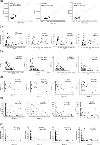
Figure 5. Heat map of variables’ correlation coefficient based on the DPSIR framework. (a) Heat map between Driving Force and Pressure variables, (b) Heat map between Driving Force and State variables, (c) Heat map between Pressure and State variables, (d) Heat map between Response and Driving Force variables, (e) Heat map between Response and Pressure variables, (f) Heat map between Response and State variables. The horizontal and vertical coordinates in the heat map are the abbreviations of the variables and the numbers are the correlation coefficients between the variables.

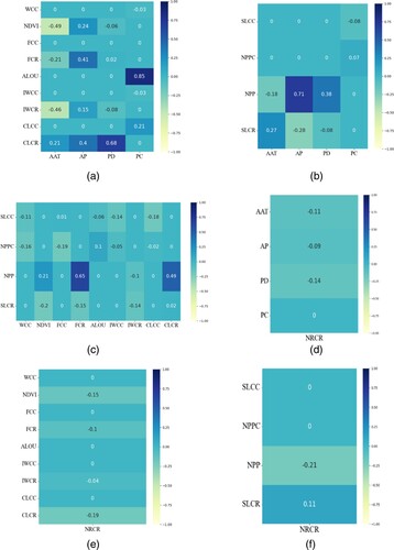
We selected variables with correlation coefficients greater than 0.2 in the confidence interval 0.01 and classified them into three grades. The refined ESDGVs and their grade are shown in Table 3. Interrelationships among goals, targets, indicators, and ESDGVs are shown in Figure 6.

Figure 6. Interrelationships among goals, targets, indicators, and EVs. The second layer in the figure is the goals layer; the third layer is the targets layer; the fourth layer is the indicators layer; and the fifth layer is the ESDGVs layer, with colours to indicate different categories. The thickness of the lines indicates the grades of the ESDGVs. The thickest lines are connected to ESDGVs of Grade I.

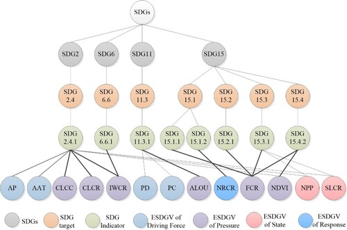
Table 3. List of refined ESDGVs for land degradation.

Component	ESDGVs for Land Degradation	Related Indicators	Grade
Driving Force	Population distribution	11.3.1: Ratio of land consumption rate to population growth rate	III
	Population change	11.3.1: Ratio of land consumption rate to population growth rate	III
	Annual precipitation	2.4.1: Proportion of agricultural area under productive and sustainable agriculture	II
	Annual average temperature	2.4.1: Proportion of agricultural area under productive and sustainable agriculture	II
Pressure	Cultivated land cover rate	2.4.1: Proportion of agricultural area under productive and sustainable agriculture	I
	Cultivated land cover change	2.4.1: Proportion of agricultural area under productive and sustainable agriculture	I
	Inland water cover rate	2.4.1: Proportion of agricultural area under productive and sustainable agriculture 6.6.1: Change in the extent of water-related ecosystems over time	I
	The area of the land occupied by the city/urban area over a period	11.3.1: Ratio of land consumption rate to population growth rate	I
	Forest cover rate	15.1.1: Forest area as a proportion of total land area 15.2.1: Progress towards sustainable forest management 15.3.1: Proportion of land that is degraded over total land area 15.4.2: Mountain Green Cover Index	I
	NDVI value	2.4.1: Proportion of agricultural area under productive and sustainable agriculture 15.4.2: Mountain Green Cover Index	I
State	NPP value	2.4.1: Proportion of agricultural area under productive and sustainable agriculture 15.3.1: Proportion of land that is degraded over total land area	III
	Cover rate of salinized land	2.4.1: Proportion of agricultural area under productive and sustainable agriculture 15.3.1: Proportion of land that is degraded over total land area	III
Response	Cover rate of nature reserves	15.1.2: Proportion of important sites for terrestrial and freshwater biodiversity that are covered by protected areas, by ecosystem type	I

4.2 Analysis

We selected a series of variables from the SDGs indicators based on a subjective analysis of existing research results, technical reports, and definitions of variables with the help of the DPSIR framework. Population distribution, Population change, Annual precipitation, Annual average temperature as anthropogenic and natural factors affecting urban development and soil health were extracted as Driving Force variables(Lewison et al. 2016; Seifollahi-Aghmiuni et al. 2022). Soil organic carbon affects vegetation productivity by affecting processes such as water infiltration, resulting in reduced crop yields (UN 2022); exposed land accelerates soil erosion; reduced water availability can affect the natural productivity of vegetation and cause a range of ecological problems(Song et al. 2020; Batunacun et al. 2019); urban sprawl can lead to soil depletion and accelerate soil sanding. Therefore, variables related to the themes of water environment, carbon stock, vegetation cover, and town expansion were extracted as Pressure. The State variables were extracted mainly from the concept of land degradation and its main manifestations, i.e. biological productivity and complexity of forests, rainfed fields, etc. (UN 2022). NPP is an intuitive variable reflecting land productivity, and secondly we also selected Salinized land Cover to reflect the level of soil erosion, which is also an important indicator of land degradation (Xie et al. 2020). Soil biodiversity, Output value of grain per unit, was selected as the Impact variable to measure the adverse effects of land degradation, since land degradation causes a reduction in biodiversity and crop yield(Wu et al. 2021). Response focuses on the development of policies and measures, for which the Nature reserves cover rate is chosen.

After the refinement, the original 21 variables were reduced to 13. Soil organic carbon and Soil biodiversity were abandoned due to difficulties in data or lack of acquisition. Output value of grain per unit was discarded due to difficulties in disaggregating the data. Variables such as forest cover change, the inland water cover change and wetland cover change do not satisfy the relevance criterion because of the low Pearson correlation coefficient between them and other variables. Grade I variables are cultivated land coverage rate, cultivated land coverage change, inland water coverage rate, the area of land occupied by urban areas, forest coverage rate, NDVI and coverage rate of nature reserves. These variables play an important role in the evolution and prevention of land degradation, their spatial data are easy to obtain and their calculation method is well established. Such ESDGVs are mostly related to land cover and depend on earth observations, especially remote sensing technology, which facilitates their data acquisition and calculation. Grade II variables include annual precipitation and annual average temperature. China has a number of meteorological stations that can collect temperature, humidity, precipitation, air pressure, wind speed and other data, which are useful for climate change, environmental and other types of research. However, these data need to be interpolated for spatial analysis and quality controlled before they can be put into use. Fortunately, there are already some highly accurate meteorological datasets available in China. Grade III variables include population distribution, population change, NPP value, and coverage rate of salinized land. Most of these variables are related to socio-economic variables or must be sampled in the field. Such data are usually counted in the form of administrative units and, thus, difficult to spatialize.

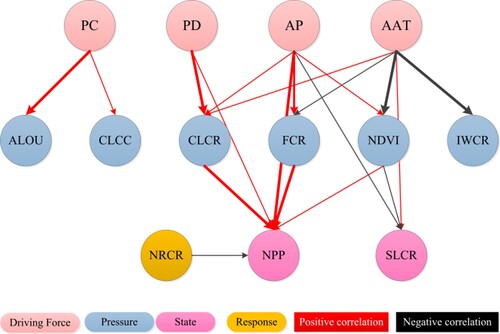
Indicators are interrelated and one ESDGV can monitor multiple indicators, as shown in Table 3. Therefore, the refined ESDGVs can not only reduce the workload without losing key information and monitor SDGs more effectively, but also show the impact mechanism of land degradation more clearly. Sorting out and analyzing these ESDGVs can find that the interaction among between them is complicated (Figure 7). In terms of climate, temperature relates to NPP through NDVI, forest and cultivated land cover indirectly; temperature can also affect the proportion of salinized land through NDVI. Precipitation promotes vegetation growth and has a positive correlation with forest, cultivated land and NDVI, which affect NPP positively. In addition, precipitation can also affect changes in saline soils directly or indirectly. In terms of human activities, population distribution has a strong positive correlation with cultivated land coverage rate, which in turn affects NPP. Population change affects the development of urbanization and the change of cultivated land. The area of nature reserves is inversely correlated with NPP, indicating that the establishment of nature reserves doesn’t play a positive role in curbing land degradation.

Figure 7. Correlation between the essential variables. Different colours represent different parts of DPSIR. Line thickness represents the strength of the correlation.

Figure 8 shows a case of the interaction between ESDGVs on the scale of 100 km × 100 km in northwest China. In this area, the precipitation is higher in the marginal areas and lower in the central and western areas. Cultivated land and NPP have been similarly distributed from 2000 to 2015. It can be concluded that there are relatively clear patterns in the spatial distribution of precipitation and arable land resources. The richness of cultivated land resources is an important indicator that reflects the progress of sustainable agriculture implementation, and is closely related to SDG2. Almost all cultivated land resources in Northwest China are concentrated in marginal areas. The cultivated land in the west and north is scarce and fragmented, reflecting a lower importance of agriculture.

Figure 8. Changes in ESDGVs that characterize land degradation. An example of annual precipitation, cultivated land coverage rate and NPP. (a), (b), (c), (d) correspond to the years of 2000, 2005, 2010, 2015, respectively.

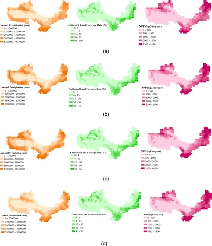
In Figure 8, the distribution of NPP is consistent with that of cultivated land and precipitation resources. Areas rich in arable land resources also have better land productivity. Protecting cultivated land resources can help curb land degradation (SDG15) but it is not the only factor affecting NPP, especially in the northeast, where NPP is high despite the scarcity of cultivated lands. The areas with high NPP are concentrated in the northern and southern edges. Vegetation in these areas grows well, indicating that the soil is healthy and land degradation is low. However, desertification is still serious in most other areas and poses a great threat to the environmental health of the region.

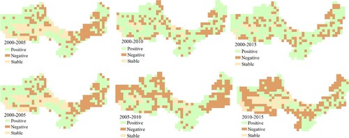
We used the Cover rate of salinized land and NPP belonging to State variables, and followed the principle of ‘1 out, all out’ to plot the land degradation trends. From Figure 9, it can be seen that the land degradation status has improved in general with the year 2000 as the base year, and the total area of deteriorated land is decreasing while the total area of improved land is increasing. However, when we compare with the previous period, the eastern region and the western region reflect a large difference. Analysing the land degradation trends in the three stages of 2000–2005, 2005–2010, and 2010–2015, it can be seen that the western region has a tendency to improve year by year, but the land status in the eastern and central regions continues to deteriorate. In the development of 2000-2015, the land degradation control in Inner Mongolia region has been effective, and the government should pay more attention to the land degradation control in Xinjiang and Gansu in the future.

Figure 9. Land degradation trends between 2000-2015, with 2000 and the previous period year as the baseline, respectively. Negative indicates an increase in salinized land cover or a decrease in NPP; Stable indicates that both salinized land and NPP are in a unchanged state; Positive refers to an improvement in land salinization and land productivity.

5. Discussion

The filtered ESDGVs ensure the conciseness of information, which is of great significance for the actual work. Because a large monitoring system means more data to be collected. The difficulty of obtaining the datasets we need due to difficulty of sampling, the high price, and the availability of data from different sources, hinders the successful implementation of monitoring. In addition, useless variables will bring redundant information for policy development and will be less efficient or even disruptive. In this study, the variables belonging to cover rate change (such as the forest cover change, the inland water cover change, wetland cover change, etc.) were proved to play a smaller role in the process of land degradation, while the variables in the distribution category (such as population distribution, forest cover, NDVI) were mostly retained, which can guide the relevant departments to consider more the spatial distribution differences of natural and human elements when formulating policies.

Although the refined variables were considered to be the most essential, we set 3 levels for ESDGVs to prioritize observations. This is because land degradation management entails huge economic costs and for economically backward areas, monitoring all variables is sometimes considered impossible (Dallimer and Stringer 2018). The variables’ grades provide an open and transparent monitoring principle that can help governments make decisions about whether some of these variables need to be observed on a priority, urgent basis given their limited budgets.

With the help of ESDGVs, some indicators can be fully monitored, for example, Forest cover rate can fully reflect the progress of SDG15.1.1 ‘Forest area as a proportion of total land area’; Forest cover rate and NDVI can together reflect the progress of SDG15.4.2 ‘Mountain Green Cover Index’. However, while some indicators cannot be fully monitored because of data acquisition and disaggregation, such as 2.4.1: Proportion of agricultural area in productive and sustainable agriculture, ESDGVs can still reflect progress on these indicators to some extent.

There are still some limitations and difficulties in the refining method presented, which are addressed in the following points for discussion.

5.1 Data acquisition

Despite the advances in earth observation technology, some data are still difficult to obtain. In this paper, we had to leave out variables, such as soil biodiversity and grain output, due to the high cost and complexity of their data acquisition. In addition to these environmental data, some socio-economic data can only be found in statistical yearbooks. These non-spatialized data based on administrative regions can hardly be integrated with other geographical data. Although there are some mature international raster data sets for demographic and economic data, their accuracy and scale are far from meeting our needs.

5.2 Interdisciplinarity

Assessing the environment itself can overlook the coupling of environmental and human activities. Therefore, sustainable development issues should be assessed through the lens of systematic observation. Human activities encompass all aspects of society and economy, and bring about complex impacts on the environment, and this paper has not been able to extend the study in this aspect due to the limitation of specialty. How to integrate the interdisciplinary knowledge needs to be further explored in future work.

5.3 Spatial and time scales

Differences in spatial scales may affect the results. The final refined variables can be of different grid sizes, which affects the correlation between them. Spatial scale effects are inevitable in spatial analyses and affect the universality of spatially sensitive ESDGVs. However, this point needs to be further tested and discussed in future work. In addition, the choice of time scale may also affect the process and results of the SDGs assessment. In this paper, we selected four time points from 2000 to 2015, and the experimental results showed good regularity. However, sometimes, a shorter time scale is needed to reveal the accelerated impact of policies or the natural environment on the evolution of the land. Therefore, we maybe need a criterion to judge and verify whether the spatial scale and temporal scale are appropriately chosen.

5.4 Applicability

Finally, the variables in this study were refined to suit the situation of the research area. This set of ESDGVs can be used to monitor northwest China or other areas with similar social, economic and environmental conditions but are not applicable to all regions.

6. Conclusion

The SDGs have received widespread attention and have been applied to a variety of fields since their inception. However, practical problems, such as interdisciplinary attributes, massive data and heavy workloads, complicate the implementation of SDGs monitoring. This paper presented a combined qualitative and quantitative method to refine the ESDGVs for land degradation and applied it to four provinces in the northwest of China. Compared to conventional observations, the ESDGVs greatly reduced the workload and made the monitoring and evaluation of regional SDGs easier to implement. The main contributions of this paper are as follows:

1. The widely used DPSIR framework was introduced into the extraction and refinement of ESDGVs to ensure the integrity of the information in the ESDGVs by simplifying variables and eliminating redundant information.

2. An EV refining method combining qualitative and quantitative approaches was proposed. This method relies on expert knowledge and observational data, adding quantitative calculations to qualitative judgments, which can help us overcome the subjectivity of traditional methods that only rely on qualitative judgment.

3. An application case based on land degradation was presented. In this paper, four provinces in northwest China were selected as experimental areas and the refining process and results of the ESDGVs based on land degradation were described, providing an example of the application of regional ESDGVs.

The applications of EVs are becoming established in other fields but are still in the initial stage in the SDGs. There are many SDG indicators beyond land degradation. Finally, we hope to add more interdisciplinary knowledge in the future when refining ESDGVs, based on which more socially and economically disaggregated datasets should be produced to flexibly study the coupling between environment and population at the grid scale. In addition, SDGs monitoring should serve the actual production, and it is necessary to establish more and deeper links with governments and stakeholders.

Acknowledgments

The authors thank the NASA team for providing MODIS data. We also thank Resource and environment science and data center for the LUCC data and meteorological data. We appreciate WorldPop for sharing demographic data.

Disclosure statement

No potential conflict of interest was reported by the author(s).

Data availability statement

The land use and land cover data presented in this study are openly available in [CNLUCC] at [10.12078/2018070201]. MODIS data can be found here [Error! Hyperlink reference not valid.]. Demographic data can be found in [https://www.worldpop.org/geodata/listing?id = 75]. The meteorological data presented in this study are openly available at [10.12078/2022082501].

Additional information

Funding

This work was supported by the key program of National Natural Science Foundation of China [grant number 41930650].

References

- Batunacun, R. Wieland, T. Lakes, Y.F. Hu, and C. Nendel. 2019. “Identifying Drivers of Land Degradation in Xilingol, China, Between 1975 and 2015.” Land Use Policy 83: 543-559. doi:10.1016/j.landusepol.2019.02.013.
- Bojinski, S., M. Verstraete, T. C. Peterson, C. Richter, A. Simmons, and M. Zemp. 2014. “The Concept of Essential Climate Variables in Support of Climate Research, Applications, and Policy.” Bulletin of the American Meteorological Society 95 (9): 1431–1433. doi:10.1175/BAMS-D-13-00047.1.
- Bradley, P., and S. Yee. 2015. “Using the DPSIR Framework to Develop a Conceptual Model: Technical Support Document.” In US Environmental Protection Agency, Office of Research and Development, Atlantic Ecology Division. Narragansett, RI.
- Chandrakumar, C., and S. J. McLaren. 2018. “Towards a Comprehensive Absolute Sustainability Assessment Method for Effective Earth System Governance: Defining key Environmental Indicators Using an Enhanced-DPSIR Framework.” Ecological Indicators 90: 577–583. doi:10.1016/j.ecolind.2018.03.063.
- Chen, J., H. Ren, W. Geng, S. Peng, and Y. E. Fanghong. 2018. “Quantitative Measurement and Monitoring Sustainable Development Goals(SDGs) with Geospatial Information.” Geomatics World 7: 1–7. doi:10.3969/j.issn.1672-1586.2018.01.001.
- Dallimer, M., and L. C. Stringer. 2018. “Informing Investments in Land Degradation Neutrality Efforts: A Triage Approach to Decision Making.” Environmental Science & Policy 89: 198–205. doi:10.1016/j.envsci.2018.08.004.
- Didan, K. MOD13A3: MODIS/Terra Vegetation Indices Monthly L3 Global 1 km SIN Grid.” In.: NASA EOSDIS Land Processes DAAC.
- Gbagir, A. M. G., C. S. Sikopo, K. K. Matengu, and A. Colpaert. 2022. “Assessing the Impact of Wildlife on Vegetation Cover Change, Northeast Namibia, Based on MODIS Satellite Imagery (2002–2021).” Sensors 22 (11): 4006. https://doi.org/10.3390/s22114006.
- Giuliani, G., P. Mazzetti, M. Santoro, S. Nativi, J. Van Bemmelen, G. Colangeli, and A. Lehmann. 2020. “Knowledge Generation Using Satellite Earth Observations to Support Sustainable Development Goals (SDG): A use Case on Land Degradation.” International Journal of Applied Earth Observation and Geoinformation 88: 102068. doi:10.1016/j.jag.2020.102068.
- Guo, H., D. Liang, F. Chen, and Z. Shirazi. 2021. “Innovative Approaches to the Sustainable Development Goals Using Big Earth Data.” Big Earth Data 5 (3):263-276. doi:10.1080/20964471.2021.1939989
- Houghton, J., J. Townshend, K. Dawson, P. Mason, J. Zillman, and A. Simmons. 2012. “The GCOS at 20 Years: The Origin, Achievement and Future Development of the Global Climate Observing System.” Weather 67 (9): 227–235. doi:10.1002/wea.1964.
- Hutchinson, M. F. 1998. “Interpolation of Rainfall Data with Thin Plate Smoothing Splines - Part I: Two Dimensional Smoothing of Data with Short Range Correlation.” Journal of Geographic Information and Decision Analysis 2 (2): 139–151.
- Jiang, L., A. Bao, G. Jiapaer, R. Liu, Y. Yuan, and T. Yu. 2022. “Monitoring Land Degradation and Assessing its Drivers to Support Sustainable Development Goal 15.3 in Central Asia.” Science of The Total Environment 807 (pt 2): 150868–13. doi:10.1016/j.scitotenv.2021.150868.
- Kussul, N., M. Lavreniuk, A. Kolotii, S. Skakun, O. Rakoid, and L. Shumilo. 2020. “A Workflow for Sustainable Development Goals Indicators Assessment Based on High-Resolution Satellite Data.” International Journal of Digital Earth 13 (2): 309–321. doi:10.1080/17538947.2019.1610807.
- Lal, R., J. Bouma, E. Brevik, L. Dawson, D. J. Field, B. Glaser, R. Hatano, et al. 2021. “Soils and Sustainable Development Goals of the United Nations (New York, USA): An IUSS perspective.” Geoderma Regional 25: e00398. doi:10.1016/j.geodrs.2021.e00398.
- Lehmann, A., J. Masò, S. Nativi, and G. Giuliani. 2020. “Towards Integrated Essential Variables for Sustainability.” International Journal of Digital Earth 13 (002): 158–165. doi:10.1080/17538947.2019.1636490.
- Lewison, R. L., M. A. Rudd, W. Al-Hayek, C. Baldwin, M. Beger, S. N. Lieske, C. Jones, S. Satumanatpan, C. Junchompoo, and E. Hines. 2016. “How the DPSIR Framework Can be Used for Structuring Problems and Facilitating Empirical Research in Coastal Systems.” Environmental Science & Policy 56: 110–119. doi:10.1016/j.envsci.2015.11.001.
- Liu, Y., W. Du, N. Chen, and X. Wang. 2020a. “Construction and Evaluation of the Integrated Perception Ecological Environment Indicator (IPEEI) Based on the DPSIR Framework for Smart Sustainable Cities.” Sustainability 12 (17): 7112. doi:10.3390/su12177112.
- Liu, L. J., Y. J. Liang, and S. Hashimoto. 2020b. “Integrated Assessment of Land-use/Coverage Changes and Their Impacts on Ecosystem Services in Gansu Province, Northwest China: Implications for Sustainable Development Goals.” Sustainability Science 15 (1): 297–314. doi:10.1007/s11625-019-00758-w.
- Lloyd, C. T., H. Chamberlain, D. Kerr, G. Yetman, L. Pistolesi, F. R. Stevens, A. E. Gaughan, et al. 2019. “Global Spatio-Temporally Harmonised Datasets for Producing High-Resolution Gridded Population Distribution Datasets.” Big Earth Data 3 (2): 108–139. doi:10.1080/20964471.2019.1625151.
- Lu, Y. L., L. Kauppi, L. Jacqueline, A. Dahl, B. Milligan, C. Patrice, F. Hinds, et al. 2015. “Marine Resource Scoping Report “Ecosystem Approach for Sustainable Management of Marine Resources.” In The Ecosystem Approach for Sustainable Management of Marine Resources. UNEP International Resource Panel Scoping Report.
- Masó, J., I. Serral, C. D. Marimon, and A. Zabala. 2020. “Earth Observations for Sustainable Development Goals Monitoring Based on Essential Variables and Driver-Pressure-State-Impact-Response Indicators.” International Journal of Digital Earth 13 (2): 217–235. doi:10.1080/17538947.2019.1576787.
- Mason, P., M. Manton, D. Harrison, A. Belward, A. Thomas, A. Dawson, A. Allali, et al. 2003. The Second Report on the Adequacy of the Global Observing System for Climate in Support of the UNFCCC. In.: GCOS.
- Masoudi, M., M. Vahedi, and A. Cerdà. 2021. “Risk Assessment of Land Degradation (RALDE) Model.” Land Degradation & Development 32 (1): 2861–2874. doi:10.1002/ldr.3883.
- Miloslavich, P., N. J. Bax, S. E. Simmons, E. Klein, W. Appeltans, O. Aburto-Oropeza, G. M. Andersen, et al. 2018. “Essential Ocean Variables for Global Sustained Observations of Biodiversity and Ecosystem Changes.” Global Change Biology 24 (6):2416-2433. doi:10.1111/gcb.14108.
- Nativi, S., M. Santoro, G. Giuliani, and P. Mazzetti. 2020. “Towards a Knowledge Base to Support Global Change Policy Goals.” International Journal of Digital Earth 13 (2): 188–216. doi:10.1080/17538947.2018.1559367.
- Nwilo, P. C., D. N. Olayinka, C. J. Okolie, E. I. Emmanuel, M. J. Orji, and O. E. Daramola. 2020. “Impacts of Land Cover Changes on Desertification in Northern Nigeria and Implications on the Lake Chad Basin.” Journal of Arid Environments 181: 104190. doi:10.1016/j.jaridenv.2020.104190.
- Omisore, A. G. 2018. “Attaining Sustainable Development Goals in sub-Saharan Africa; The Need to Address Environmental Challenges.” Environmental Development 25: 138–145. doi:10.1016/j.envdev.2017.09.002.
- Pellens, N., E. Boelee, J. M. Veiga, L. E. Fleming, and A. Blauw. 2021. “Innovative Actions in Oceans and Human Health for Europe.” Health Promotion International 2021: 1–11. doi:10.1093/heapro/daab203.
- Plag, H. P., and S. A. Jules-Plag. 2020. “A Goal-Based Approach to the Identification of Essential Transformation Variables in Support of the Implementation of the 2030 Agenda for Sustainable Development.” International Journal of Digital Earth 13 (2): 166–187. doi:10.1080/17538947.2018.1561761.
- Reyers, B., M. Stafford-Smith, K. H. Erb, R. J. Scholes, and O. Selomane. 2017. “Essential Variables Help to Focus Sustainable Development Goals Monitoring.” Current Opinion in Environmental Sustainability 26-27: 97–105. doi:10.1016/j.cosust.2017.05.003.
- Riva, M. J., I. N. Daliakopoulos, S. Eckert, E. Hodel, and H. Liniger. 2017. “Assessment of Land Degradation in Mediterranean Forests and Grazing Lands Using a Landscape Unit Approach and the Normalized Difference Vegetation Index.” Applied Geography 86: 8–21. doi:10.1016/j.apgeog.2017.06.017.
- Rosenstock, T. S., C. Lamanna, S. Chesterman, J. Hammond, S. Kadiyala, E. Luedeling, K. Shepherd, B. DeRenzi, and M. T. V. Wijk. 2017. “When Less is More: Innovations for Tracking Progress Toward Global Targets.” Current Opinion in Environmental Sustainability, 54–61. doi:10.1016/j.cosust.2017.02.010.
- Sayl, K. N., S. O. Sulaiman, A. H. Kamel, N. S. Muhammad, J. Abdullah, and N. Al-Ansari. 2021. “Minimizing the Impacts of Desertification in an Arid Region: A Case Study of the West Desert of Iraq.” Advances in Civil Engineering (5580286): 1–12. doi:10.1155/2021/5580286.
- Scharlemann, J. P. W., R. C. Brock, N. Balfour, C. Brown, N. D. Burgess, M. K. Guth, D. J. Ingram, et al. 2020. “Towards Understanding Interactions Between Sustainable Development Goals: The Role of Environment–Human Linkages.” Sustainability Science 15: 1573–1584. doi:10.1007/s11625-020-00799-6.
- Seifollahi-Aghmiuni, S., Z. Kalantari, G. Egidi, L. Gaburova, and L. Salvati. 2022. “Urbanisation-driven Land Degradation and Socioeconomic Challenges in Peri-Urban Areas: Insights from Southern Europe.” Ambio 51 (6): 1446–1458. doi:10.1007/s13280-022-01701-7.
- Sena, A., and K. Ebi. 2021. “When Land Is Under Pressure Health Is Under Stress.” International Journal of Environmental Research and Public Health 18 (136), doi:10.3390/ijerph18010136.
- Senanayake, S., B. Pradhan, A. Huete, and J. Brennan. 2022. “Spatial Modeling of Soil Erosion Hazards and Crop Diversity Change with Rainfall Variation in the Central Highlands of Sri Lanka.” Science of the Total Environment 806 (Pt 2): 150405. doi:10.1016/j.scitotenv.2021.150405.
- Sims, N. C., G. J. Newnham, J. R. England, J. Guerschman, S. J. D. Cox, S. H. Roxburgh, R. A. Viscarra Rossel, S. Fritz, and I. Wheeler. 2021. “ Good Practice Guidance.” In SDG Indicator 15.3.1, Proportion of Land That Is Degraded Over Total Land Area. Version 2.0..” In. Bonn, Germany: United Nations Convention to Combat Desertification.
- Song, X., J. Liao, X. Xue, and Y. H. Ran. 2020. “Multi-Sensor Evaluating Effects of an Ecological Water Diversion Project on Land Degradation in the Heihe River Basin, China.” Frontiers in Environmental Science 8. doi:10.3389/fenvs.2020.00152.
- Tóth, G., T. Hermann, M. R. D. Silva, and L. Montanarella. 2018. “Monitoring Soil for Sustainable Development and Land Degradation Neutrality.” Environmental Monitoring and Assessment 190 (2): 57. doi:10.1007/s10661-017-6415-3.
- Tucker, C., and J. Pinzon. 2018. “Satellite Mapping of Land Degradation in Senegal, Uganda, Kenya, and Tanzania.” In IGARSS 2018 – 2018 IEEE International Geoscience and Remote Sensing Symposium.
- Turak, E., J. Brazill-Boast, T. Cooney, M. Drielsma, J. DelaCruz, G. Dunkerley, M. Fernandez, et al. 2017. “Using the Essential Biodiversity Variables Framework to Measure Biodiversity Change at National Scale.” Biological Conservation 213 (Pt.B): 264–271. doi:10.1016/j.biocon.2016.08.019.
- UN. 2022. “SDG Indicators Metadata repository.” In, edited by Department of Economic and Social Affairs.
- Wang, T., G. Giuliani, A. Lehmann, Y. Jiang, X. Shao, L. Li, and H. Zhao. 2020. “Supporting SDG 15, Life on Land: Identifying the Main Drivers of Land Degradation in Honghe Prefecture, China, Between 2005 and 2015.” ISPRS International Journal of Geo-Information 9 (12): 710. doi:10.3390/ijgi9120710.
- Wang, X. Y., C. Q. Song, C. X. Cheng, S. J. Ye, and S. Shen. 2021. “Cross-national Perspectives on Using Sustainable Development Goals (SDGs) Indicators for Monitoring Sustainable Development: A Database and Analysis.” Chinese Geographical Science 31 (4): 600–610. doi:10.1007/s11769-021-1213-9.
- Wei, O. Y., Z. M. Lian, X. Hao, X. Gu, F. Hao, C. Lin, and F. Zhou. 2018. “Increased Ammonia Emissions from Synthetic Fertilizers and Land Degradation Associated with Reduction in Arable Land Area in China.” Land Degradation & Development 29: 3928–3939. doi:10.1002/ldr.3139.
- Wu, Y., D. M. Chen, M. Saleem, B. Wang, S. J. Hu, M. Delgado-Baquerizo, and Y. F. Bai. 2021. “Rare Soil Microbial Taxa Regulate the Negative Effects of Land Degradation Drivers on Soil Organic Matter Decomposition.” Journal of Applied Ecology 58 (8): 1658–1669. doi:10.1111/1365-2664.13935.
- Wunder, S., and R. Bodle. 2019. “Achieving Land Degradation Neutrality in Germany: Implementation Process and Design of a Land use Change Based Indicator.” Environmental Science & Policy 92: 46–55. doi:10.1016/j.envsci.2018.09.022.
- Xie, H. L., Y. W. Zhang, Z. L. Wu, and T. G. Lv. 2020. “A Bibliometric Analysis on Land Degradation: Current Status, Development, and Future Directions.” Land 9 (1): 28. doi:10.3390/land9010028.
- Xu, K. P., Y. Y. Chi, J. J. Wang, R. F. Ge, and X. H. Wang. 2021. “Analysis of the Spatial Characteristics and Driving Forces Determining Ecosystem Quality of the Beijing–Tianjin–Hebei Region.” Environmental Science and Pollution Research volume 28: 12555-12565. doi:10.1007/s11356-020-11146-8.
- Xu, X. L., J. Y. Liu, S. W. Zhang, R. D. Li, C. Z. Yan, and S. X. Wu. 2018. “China’s Multi-Period Land Use Land Cover Remote Sensing Monitoring Dataset (CNLUCC).” In, Edited by Data Registration and Publishing System of the Resource and Environmental Science Data Center of the Chinese Academy of Sciences.
- Zakerinejad, R., and M. Masoudi. 2019. “Quantitative Mapping of Desertification Risk Using the Modified MEDALUS Model: A Case Study in the Mazayejan Plain, Southwest Iran.” AUC Geographica 54: 232–239. doi:10.14712/23361980.2019.20.
- Zhang, Y. Z., Y. F. Hu, Y. Q. Han, and S. Zhan. 2021. “Spatial Distributions and Evolutions of Global Major Ecological Degradation Regions and Research Hotspot Regions.” Acta Ecologica Sinica 41 (1000-0933): 7599. doi:10.5846/stxb202002150260.
- Zheng, D., and Y. Yin. 2010. “Eco-reconstruction in Northwest China.” In Water and Sustainability in Arid Regions, edited by G. Schneier-Madanes, and M. F. Courel. Dordrecht: Springer. doi:10.1007/978-90-481-2776-4_1.