Developing a new red band–SEVI–blue band (RSB) enhancement method for recognition the extra-high-voltage transmission line corridor in green mountains

ABSTRACT

Monitoring the extra-high-voltage transmission line corridor (EHVTLC) in mountains is critical for safe smart-grid operation. However, the transmission lines are so narrow that they are difficult to recognize using multispectral satellite images with a spatial resolution of 10 m. In this study, we developed a new method using the red band–shadow-eliminated vegetation index (SEVI)–blue band (RSB) composite image to enhance the EHVTLC in green mountains (named RSB-enhancement method). Using this method, the EHVTLC becomes evident in the false-color synthesis of the RSB composite of the Sentinel-2 image. Then, we recognized and extracted approximately 342.45 km of the EHVTLC in a mountainous region of Fuzhou City, China, including a 46.73 km three-parallel-lane segment of 1000 kV and a 295.72 km two-parallel-lane segment of 500 kV. Spatial analysis shows that the SEVI mean difference between the EHVTLC and the buffer zone reaches approximately 10%, and three landslides and 2.66 km² soil erosion reside in the buffer zone which area is approximately 73.67 km². Finally, the RSB-enhancement method can be used in other satellite images with spatial resolutions of greater than 10 m for enhancement and recognition the transmission line corridors in green mountains.

KEYWORDS:

• Enhancement method
• shadow-eliminated vegetation index (SEVI)
• transmission line lane (TLL)
• green mountains
• soil erosion

1. Introduction

In the modern age, electricity provides vital energy to maintain our ecosystem. It is critical to monitor the fundamental infrastructure for the secure and sustainable operation of smart grids, such as power stations, converting substations, power lines, and pylons (Matikainen et al. 2016; Yang et al. 2020; Gao et al. 2022). Transmission line monitoring includes two aspects: power line components and surrounding objects, such as lines (Chen et al. 2016; Hui et al. 2018; Yetgin and Gerek 2018), insulators (Reddy, Chandra, and Mohanta 2013; Wu and An 2014; Ling et al. 2019), catenary split pins (Zhong et al. 2019), pylons or towers (Xie et al. 2014), support components (Liu et al. 2020; Lyu et al. 2020), and surrounding trees (Ahmad et al. 2013). Traditionally, it depends on field surveys and airborne or unmanned aerial vehicle (UAV) monitoring (Yan et al. 2007; Whitworth et al. 2001; Song et al. 2020), which provide super-high-resolution images or close observation. In recent years, interest in multi-source data aimed at the inspection of transmission lines and surrounding vegetation has bloomed. The corresponding data used for transmission lines have been reviewed (Matikainen et al. 2016; Yang et al. 2020), including optical aerial images (Li et al. 2012; Jones and Earp 2001; Sun et al. 2006; Song and Li 2014), synthetic aperture radar (Deng et al. 2012), thermal (Fernandes 1989), laser or lidar (Axelsson 1999; Zhang et al. 2019), and land-based mobile surveys (Liang et al. 2014; Kaartinen et al. 2015). For the underlying vegetation detection, the integration of airborne laser scanner data and aerial images was used as a method of regular inspection to decide what trees should be cut (Liu et al. 2007; Kobayashi et al. 2009; Mills et al. 2010; Li et al. 2012; Ahmad et al. 2013).

Power line extraction is a research hotspot. One basic workflow generally includes two steps: the retrieval of candidate power line pixels and line extraction from the candidates (Yan et al. 2007; Zhao et al. 2019). A wide range of techniques to detect linear features in images have been developed in the past several decades, including mathematical morphology, Radon Transform (Radon 1986; Murphy 1986; Zhang and Couloigner 2007; Chen et al. 2016), Hough Transform (Axelsson 1999; Mukhopadhyay and Chaudhuri 2015; Guan et al. 2016), Canny algorithm (Canny 1986; Li 2020), multi-resolution techniques, template matching, dynamic programming, classification-based feature extraction (Quackenbush 2004), artificial intelligence of machine learning and deep learning (Zhang et al. 2020), e.g. Random Forest (Kim and Sohn 2013), JointBoost Classifier (Guo et al. 2015), and Convolutional Neural Networks (Luo, Yu, and Yang 2021). In addition, enhancement methods have been used to highlight power lines (Ye et al. 2018). However, monitoring using super-high spatial resolution images covers a small area each time or requires a great deal of manpower to survey a large area, as the power line facilities are distributed in remote or harsh environments and are generally difficult to reach. Moreover, transmission line facilities, just as high-speed railways, highways, and oil and gas pipelines, face risks from soil erosion, fire, flooding, landslides, earthquakes, storms, and ice. Monitoring the transmission line distribution is a precondition for regional hazard risk evaluation. Apparently, traditional methods using field surveys, airborne methods, or UAV cannot meet the requirements for transmission line monitoring in regional areas. Conventionally, these potential natural hazards or risks have been studied and evaluated using satellite images with medium-high spatial resolution.

However, the detection of power lines from satellite images with a spatial resolution of 10 m has been very rare until now, because the diameter of the lines is only approximately 30 mm, and power line monitoring is influenced by many factors, such as spatial resolution of images, weather conditions, topographic effects, solar angles, and complex background land covers. Therefore, the recognition of power lines from a surrounding forest environment in a region has become a great challenge, especially in mountainous areas where topographic effect is an added disturbance to transmission line detection, e.g. self-shadows and cast shadows (Giles 2001; Jiang et al. 2019). It is more difficult to detect the transmission lines from a topographic shadow than from a sunny area because direct solar irradiance is lacking in shadowed area. Therefore, we should consider enhancing the weak target of the power lines and removing topographic effect simultaneously before extracting it in mountainous areas.

In addition, to improve electricity transmission efficiency and effectiveness, extra-high-voltage (EHV) transmission has been developed, which has the advantages of high transmission capacity, long transmission distance, decreased line loss, reduced land area used for the line corridor, and reduced cost. A power line is a conductor of fabricated aluminum cable steel reinforcement (ACSR), which has a diameter of approximately 30 mm, and the overhead ground wire is a stranded galvanized steel wire (SGSW) with a diameter of approximately 10 mm. The EHV transmission uses a set of ACSR and an overhead ground wire mounted on the pylons, which form a transmission line lane (TLL). The power lines quantity and structure of the EHV transmission depend on the voltage. For example, each lane of 500 kV has three phases, in which each phase has a quadrangle bundle structure of lines. The 500+ kV EHV transmission line corridor (EHVTLC) typically consists of two- or three-lanes. Therefore, the possibility of detection by satellite is increased for the EHVTLC, owing to the enlarged surface area of the power lines in a pixel of a remotely sensed image.

The objectives of this study are to develop a new method for enhancing and recognizing the EHVTLC of 500+ kV distributed in a large area of green mountains, using Sentinel-2 multispectral images, and to conduct spatial analysis and hazard risk evaluation for the extracted EHVTLC on a regional scale.

2. Study area and materials

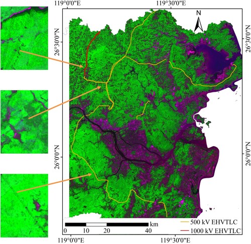
The study area is Fuzhou City in Southeast China (Figure 1), with land elevation ranging from 0 m to 1672 m with a mean of approximately 339 m and a slope ranging from ∼1° to 68° with a mean of approximately 15°. The major land cover in this area is mountainous forest with prominent topographic effect. We downloaded four scenes of Sentinel-2 Level 1C multispectral images (top-of-atmosphere apparent reflectance) from the European Space Agency (ESA) (Available online: https://scihub.copernicus.eu/dhus/#/home (accessed on 23 November 2022)) and downloaded the corresponding 30 m Advanced Spaceborne Thermal Emission and Reflection Radiometer Global Digital Elevation Model Version 2 (ASTER GDEM V2) from the Geospatial Data Cloud site, Computer Network Information Center, Chinese Academy of Sciences (Geospatial Data Cloud. Available online: http://www.gscloud.cn (accessed on 22 February 2022)). The acquired date, sun elevation and azimuth, and cloud percentages of the images used are listed in Table 1. In addition, we collected soil erosion and geologic hazard data from 2021. We also collected some material samples, including the EHV transmission line of the ACSR (JL/G1A-300/25) with a diameter of 28 mm, overhead ground wire of the SGSW with a diameter of 11 mm, and angle steel.

Figure 1. Study area location and the Sentinel-2 images (red–green–blue (RGB) composite): Red triangle is the Lili converting substation, and red rectangle is a subarea.

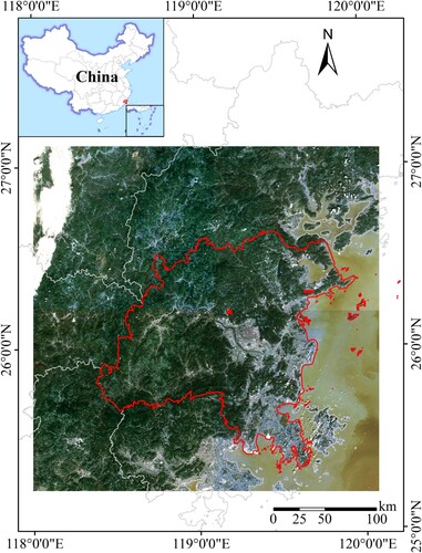
Table 1. Tile number field, acquired date, sun elevation and azimuth, and cloud percentage of the Sentinel-2 images.

Tile number field	Acquired date	Sun elevation (°)	Sun azimuth (°)	Cloud percentage (%)
T50RPP	26 October 2017	49.19	157.59	0
T50RPQ	26 October 2017	48.34	157.91	1.52
T50RQP	26 October 2017	49.53	158.98	0.03
T50RQQ	26 October 2017	48.67	159.29	0.06

3. Methods

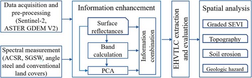
The procedure includes data acquisition and pre-processing, spectral measurement, information enhancement, EHVTLC extraction and evaluation, and spatial analysis (Figure 2). In the information enhancement step, we used band calculation, principal component analysis (PCA), and information combination to highlight the EHVTLC.

Figure 2. Flow chart for the extra-high-voltage transmission line corridor (EHVTLC) study: ASTER GDEM V2 is Advanced Spaceborne Thermal Emission and Reflection Radiometer Global Digital Elevation Model Version 2, ACSR is aluminum cable steel reinforced, SGSW is stranded galvanized steel wire; conventional land covers include water, soil, road, construction land (concrete), grass, shrub, bamboo, fir, red pine, and broad-leaved forest; surface reflectances include the frequently used wavebands of the RGB and near-infrared (NIR); PCA is principal component analysis, SEVI is shadow-eliminated vegetation index, and Topography includes elevation and slope.

3.1 Spectral measurement

The surface reflectances of the samples were measured using a FieldSpec 4 spectroradiometer on 10 August 2022, under clear sky conditions. The samples included the EHV transmission line of the ACSR, overhead ground wire of the SGSW, angle steel, and conventional underlying land covers such as water, soil, road, construction land (concrete), grass, shrub, bamboo, fir, red pine, and broad-leaved forest (Table 2). Considering the mixed species of broad-leaved trees in the subtropical mountains, we used the averaged value of the measured reflectance of the eucalyptus, camphor tree, Ficus microcarpa, and mango tree.

Table 2. Samples of the ACSR, SGSW, angle steel, and conventional land covers of water, soil, road, concrete, and vegetations.

Types	1	2	3	4
Non-vegetation
	ACSR (brand new)	ACSR (used and discarded)	SGSW (used and discarded)	Angle steel
	Water	Soil	Road	Concrete
Vegetations				/
	Grass	Reed	Dicranoteris dichotoma	/
				/
	Bamboo	Fir	Red pine	/
	Eucalyptus	Camphor tree	Ficus Microcarpa	Mango tree

3.2 Image pre-processing

The surface reflectances of the frequently used 10 m wavebands of the red–green–blue (RGB, Band 4,3,2) and near-infrared (NIR, Band 8) of the Sentinel-2 image were obtained after atmospheric correction using the Sen2cor module developed by the ESA.

3.3 Information enhancement

3.3.1. Band calculation

As a preferential band calculation, the frequently used vegetation indices were selected firstly, e.g. the ratio vegetation index (RVI) (Jordan 1969) and normalized difference vegetation index (NDVI) (Rouse et al. 1974). Supposed that the removal of topographic effect can enhance the TLL in rugged mountains, the shadow-eliminated vegetation index (SEVI) was also selected because of its high performance in removing topographic effect in mountains, such as Wuyishan (Jiang and Zhou 2020; Jiang and Wu 2021). The calculation methods are given in Equations (1)–(3). For SEVI, the adjustment factor is calculated using the block information entropy algorithm (BIE-algorithm) (Jiang et al. 2022a). First, the Sentinel-2 image is divided into blocks (or grids) of 6 km × 6 km, and the corresponding DEM is also divided into blocks. Next, the slope of the DEM blocks is calculated, and the steep blocks with the 5% highest slope mean are selected. Then, Equations (4)–(7) are used to determine the target block that achieves the highest entropy for the SEVI information. Finally, the adjustment factor value of the target block ($f_s$) is used to calculate the SEVI result. (1) $\mathrm{RVI}={\displaystyle \frac{{\rho }_{nir}}{{\rho }_r}}$(1) (2) $\mathrm{NDVI}={\displaystyle \frac{({\rho }_{nir}-{\rho }_r)}{({\rho }_{nir}+{\rho }_r)}}$(2) (3) $\mathrm{SEVI}={\displaystyle \frac{{\rho }_{nir}}{{\rho }_r}+f(\mathrm{\Delta })\cdot {\displaystyle \frac{1}{{\rho }_r}=\mathrm{RVI}+f(\mathrm{\Delta })\cdot \mathrm{SVI}}}$(3) (4) $H=-{\displaystyle \frac{{\sum }_{i=1}^n{p}_i\cdot \ln (p_i)}{\ln (n)}}$(4) (5) $p_i={\displaystyle \frac{x_i}{{\sum }_{i=1}^n{x}_i},\sum _{i=1}^n{p}_i=1,0<p_i<1}$(5) (6) $f_b=\mathrm{argmax}(H),f(\mathrm{\Delta })\in (0.001,1.000)$(6) (7) $f_s=\mathrm{argmax}(H_b),f(\mathrm{\Delta })\in (f_{bj},j=1,\dots ,m)$(7) where ${\rho }_{nir}$ and ${\rho }_r$ are the surface reflectances of the NIR and red bands, respectively, $f(\mathrm{\Delta })$ is the adjustment factor, SVI is the shadow vegetation index, $H$ is the information entropy of SEVI in a block, $p_i$ is the percentage of a SEVI pixel value in a selected block, $x_i$ is a pixel value of SEVI, $n$ is the number of pixels in a selected block, $f_b$ is an optimized adjustment factor for a block, $f_s$ is the final adjustment factor for an entire scene, $H_b$ is the maximum information entropy of SEVI in a block, and $m$ is the number of selected steep blocks in an entire scene.

3.3.2. PCA calculation

The surface reflectances of the RGB and NIR wavebands and the vegetation indices of the RVI, NDVI, and SEVI were used in PCA, which is a useful technique for feature extraction and data reduction (Abdel-Qader et al. 2006; Pal, Majumdar, and Bhattacharya 2007). First, the surface reflectances of the four original wavebands were calculated to determine which component could highlight the EHVTLC. Then, the selected waveband reflectance and vegetation index, which show potential advantage in the EHVTLC recognition, were used together in the further PCA study.

3.3.3. Information combination

Optimal band combination for false-color synthesis is useful for highlighting the target (Amer, Kusky, and Ghulam 2010; Zhang et al. 2021; Wu et al. 2021). Considering the original spectral bands, PCA components, and vegetation indices, we selected the information that achieved higher sensitivity to the EHVTLC than the others to form a novel false-color synthesis to highlight the EHVTLC.

3.4. EHVTLC extraction and analysis

Using the enhanced image, we attempted to automatically extract the EHVTLC. The methods included edge detection using the Canny algorithm, line detection using the Radon Transform and the Standard Hough Transform, and classification using the Random Forest Classifier. Considering that the performance of automatic detectors varied significantly across the images, specifically the weak target of the EHVTLC, manual extraction was also used as the final solution and benchmark. For manual extraction, we created a line shape using ArcCatalog and edited it in ArcMap based on the enhanced image. Each lane of the transmission lines was set as a line at which the location error was controlled within a pixel. The pylons were used as connecting points for the line drawing.

As for the extraction performance evaluation, we used three methods of field survey, pylon verification, and TLL verification. In field survey, we investigated the power lines amount and structure of a 500 kV segment near the Lili converting substation. For pylon verification, we checked the pylon pixels between the enhanced image and RGB composite of the Sentinel-2 and Google Earth images. The pylon pixel has a high reflectance in optical wavebands because the pylon mainly consists of angle steel and concrete base. For TLL verification, we used Google Earth images to confirm the extracted results.

After extraction, the buffer zone was set at 100 m width along the edge lines of the EHVTLC. Then, the data of elevation, slope, SEVI, soil erosion, and geologic hazard were used in the spatial analysis, which may provide us with important information for early warning of a natural hazard risk.

4. Results

4.1. Measured surface reflectances

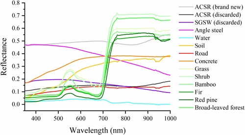
The measured spectral reflectances of the ACSR, SGSW, angle steel, and conventional underlying land covers are displayed in the spectral wavelength range of 350–1000 nm (Figure 3). The ACSR shows a relatively stable reflectance in which the mean of the brand new is approximately 0.49, higher than that of the used and discarded of approximately 0.14. The reflectance of the used and discarded SGSW shows a decline from approximately 0.20 to 0.09, and that of angle steel also decreases from nearly 0.47 to 0.23. Vegetation, including grass, shrub, bamboo, red pine, fir, and broad-leaved forest, shows distinctive characteristics of high reflectance above 0.50 in the NIR band, and relatively low reflectances ranging from approximately 0.05–0.25 in the RGB wavebands. Soil and concrete show a medium and increasing reflectance, whereas water shows a low reflectance approximately 0.03. In addition, the reflectance distribution of road is similar to that of the used and discarded ACSR. Clearly, the spectral reflectance characteristics of the ACSR and SGSW are different from those of vegetation. Specifically, the reflectance gap between the brand-new ACSR and vegetation is evident in the blue and red bands, which indicates that these bands have potential advantage in the enhancement and recognition of the EHVTLC when the underlying environment is flourish green vegetation.

Figure 3. Spectral reflectances of the ACSR, SGSW, angle steel, and conventional land covers of water, soil, road, concrete, and vegetations.

4.2. EHVTLC enhancement

It is difficult to recognize the TLL from the 10 m Sentinel-2 multispectral images (Figure 4(a,b)) and the single band images (Figure 4(c–f)). However, the optical wavebands of the blue, green and red (Figure 4(c–e)), and the true color synthesis of the RGB composite (Figure 4(a)) show a slight trace of the TLL, respectively. These phenomena indicate that the RGB wavebands are more sensitive to the TLL than the NIR band, which is in accordance with the surface reflectance gap between the RGB wavebands and the NIR band in Section 4.1. As for the PCA of the RGB and NIR wavebands, there is not one component that can highlight the TLL.

Figure 4. A Sentinel-2 sample area for transmission line lane (TLL) enhancement and comparison: (a) RGB composite, (b) NIR–red–green (NRG) composite, (c–f) surface reflectances of the blue, green, red, and NIR wavebands, (g) ratio vegetation index (RVI), (h) normalized difference vegetation index (NDVI), (i) SEVI, (j) third PCA component, (k) red band–SEVI–blue band (RSB) composite, and (l) SEVI–red band–blue band (SRB) composite.

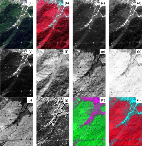
In the band calculation results, the SEVI achieves a higher enhancement performance than the RVI and the NDVI (Figure 4(g–i)), showing continual and evident transmission line corridors in a background of overall flat feature with relief impressions drastically removed, e.g. the one-lane, two-parallel-lane, and three-parallel-lane (Figure 4(i) and Figure 5(e–h)). In some segments, two corridors locate closely as two sets of two-parallel-lane (Figure 5(g)) or two sets of three-parallel-lane (Figure 5(h)). However, the corridor is disturbed by topographic effect in the RVI (Figure 4(g) and Figure 5(a–d)), while it is depressed in the NDVI (Figure 4(h)). Therefore, we selected the SEVI as a preliminary result which was used in the further PCA and the information combination.

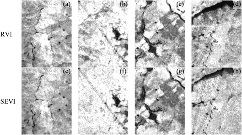
Figure 5. Transmission line corridor types and topographic effect: (a) and (e) one-lane corridor, (b) and (f) two-parallel-lane corridor, (c) and (g) two-corridor as two sets of two-parallel-lane, and (d) and (h) three-parallel-lane corridor and two-corridor as two sets of three-parallel-lane; (a)–(d) RVI with topographic effect, and (e)–(h) SEVI removed topographic effect.

Considering the wavebands and vegetation indices together, we used the SEVI, red band, and blue band to form a SEVI–red band–blue band (SRB) information combination for the PCA again and the false-color synthesis. The PCA of the SRB revealed that the third component is better for revealing the TLL than the other two components (Figure 4(j)), however, the construction land, road, and terraced fields are evident and interfere with the TLL. In the false-color synthesis, an image of the red band–SEVI–blue band (RSB) composite shows the TLL prominently in a flat background of green vegetation and pink non-vegetation (Figure 4(k)), which is helpful for visual recognizing the TLL. However, in the SRB composite image (Figure 4(l)), the TLL appears less evident than that in the RSB composite. Ultimately, the false-color synthesis of the RSB composite was selected and named as RSB-enhancement method.

4.3. Extracted EHVTLC

The EHVTLC is difficult to extract automatically using the algorithms of Canny, Radon Transform, Standard Hough Transform, and Random Forest Classifier. The noises from road, construction land, and terraced fields, are easily detected and mixed, owing to the weak target of the TLL. Therefore, we extracted the EHVTLC manually from the RSB-enhanced image. Ultimately, 342.45 km of the EHVTLC was extracted, which includes a 46.73 km three-parallel-lane segment of 1000 kV and a 295.72 km two-parallel-lane segment of 500 kV. However, 5.36 km was missed, which was underlying non-vegetation, such as water, terraced fields, roads, and construction land, and 0.43 km was missed owing to cloud. The 1000 kV is distributed as a two-corridor (two sets of three-parallel-lane) in red line of approximately 23.37 km, and the 500 kV is distributed in yellow line as a two-corridor (two sets of two-parallel-lane) of approximately 42.41 km and a two-parallel-lane corridor of approximately 210.90 km (Figure 6).

Figure 6. RSB-enhanced image and extracted EHVTLC: Red line is 1000 kV distributed as two-corridor (two sets of three-parallel-lane), and yellow line is 500 kV distributed as two-parallel-lane corridor and two-corridor (two sets of two-parallel-lane).

In extraction performance evaluation, the surveyed EHVTLC segment is three lanes (a two-parallel-lane and a one-side-lane, Figure 7(a)) of 500 kV with a quadrangle bundle structure of lines in each phase (Figure 7(b)), which verified our enhanced TLL in the RSB composite image (Figure 7(c)). In particular, the one-side-lane mounted on the pylon left side was confirmed (Figure 7(a,c,f)). In addition, the white pixels of pylons are easily recognized from the RGB composite of the Sentinel-2 image and the Google Earth image (Figure 7(e,f) and Figure 8(a,c)). Correspondingly, the pylons in the RSB composite are evident with bright pink or dark colors (Figure 7(c) and Figure 8(b)). Finally, the TLL was observed and confirmed in the Google Earth images (Figure 7(f) and Figure 8(c)), which is in accordance with our enhanced TLL (Figure 7(c) and Figure 8(b)). In a word, the total extracted EHVTLC was confirmed using pylons and the TLLs in the Google Earth images.

Figure 7. A 500 kV segment of three lanes (a two-parallel-lane and a one-side-lane) near the Lili converting substation: (a) pylons and transmission lines, (b) lines structure in each phase, (c) RSB composite of the Sentinel-2, (d) SEVI of the Sentinel-2, (e) RGB composite of the Sentinel-2, and (f) RGB composite of the Google Earth image.

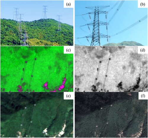
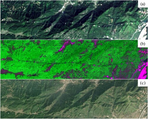
Figure 8. TLL in a subarea: (a) RGB composite of the Sentinel-2, (b) RSB composite of the Sentinel-2, and (c) RGB composite of the Google Earth image.

4.4. Spatial analysis

The extracted EHVTLC is distributed in an elevation range from 11 m to 967 m with a mean of 470 m, a slope from 0° to 66.6° with a mean of 18.5°, and a graded SEVI from 0.029 to 0.992 with a mean of 0.416 (Figure 9(a–c) and Table 3). The distribution characteristics of the buffer zone are similar to those of the EHVTLC (Figure 9(d–f) and Table 3). However, the SEVI mean difference between the EHVTLC and the buffer zone reaches approximately 10%, which discriminates them. In addition, the buffer zone area is approximately 73.67 km², where the soil erosion area occupies approximately 2.66 km², that is, a soil erosion rate of 3.61% (Figure 10). The soil erosion area is located mainly in the south and northwest segments of the buffer zone (Figure 10) and shows different distribution characteristics of a much lower elevation mean of 293 m and a higher slope mean of 20.3° (Figure 9(g,h) and Table 3). The SEVI distribution characteristics of soil erosion area were not evaluated because of the temporal mismatch between the Sentinel-2 image and the soil erosion data. As for the geologic hazard, only three landslides reside in the buffer zone, located at elevations of 238, 525, and 513 m on slopes of 9.5°, 10.2°, and 10.4°, respectively (Figure 10).

Figure 9. Histogram of the elevation, slope, and SEVI for the extracted EHVTLC, buffer zone, and soil erosion area: (a–c) EHVTLC, (d–f) buffer zone, and (g–h) soil erosion area in the buffer zone.

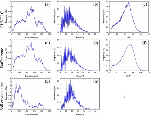
Figure 10. Soil erosion and geologic hazards in the buffer zone.

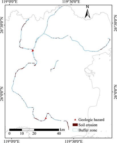
Table 3. Minimum, maximum and mean of the elevation, slope, and SEVI for the extracted EHVTLC, buffer zone, and soil erosion area.

Object	Indicator	Minimum	Maximum	Mean
EHVTLC	Elevation (m)	11	967	470
	Slope (°)	0	66.6	18.5
	SEVI	0.029	0.992	0.416
Buffer zone	Elevation (m)	9	1017	447
	Slope (°)	0	67.2	19.0
	SEVI	0.027	1.000	0.456
Soil erosion area	Elevation (m)	10	898	293
	Slope (°)	0	66.7	20.3
	SEVI	/	/	/

5. Discussions

5.1. Advantages and limitations of the RSB-enhancement method

Remote sensing monitoring level of transmission line corridor is important for the sustainable development of smart grids. However, it is a significant challenge to recognize the corridor from a large mountainous area because the transmission lines are a weak target. Specifically, it is difficult to detect the corridor using the Sentinel-2 multispectral image, let alone the ACSR of diameter approximately 30 mm. As a mixed pixel of a set of the ACSR and underlying land covers, the TLL shows a merged reflectance that depends on the amount of ACSR and type of underlying land cover. Theoretically, the reflectance characteristic of the ACSR is similar to that of non-vegetation underlying land covers, such as water, soil, roads, and concrete; thus, it is difficult to distinguish the ACSR from the underlying background of non-vegetation using optical satellite images. The characteristic reflectance difference between the ACSR and the underlying vegetation is remarkable in theory; however, the area percentage of the ACSR in a pixel is so small that the mixed pixel shows a slightly increased reflectance in the blue, red, and green bands compared to the pure pixels of vegetation. Therefore, we proposed the RSB-enhancement method to enhance the TLL using the Sentinel-2 images. The RSB information combination is an image fusion method (Xiao et al. 2020) that considers the reflectance gap between the ACSR and green vegetation in the red and blue bands and the high performance of the SEVI in enhancing the TLL and in removing topographic effect in rugged mountains (Jiang et al. 2022b). Enhancement of the TLL is a new feature of the SEVI, as it is composed of the RVI and SVI, which use the red band as the denominator. Therefore, the SEVI is suitable for enhancing the EHVTLC distributed on rugged mountains. Finally, the false-color synthesis of the RSB composite integrates the advantages of the SEVI, blue band, and red band; thus, it is a method of high performance in enhancing the EHVTLC on green mountains. The other advantages of the RSB-enhancement method include simple operation of band calculation and composition, and low cost in acquiring images covering a large area. For example, a free Sentinel-2 image covers 10,000 km² (Table 4).

Table 4. Advantages and limitations of the RSB-enhancement method.

	Advantages	Limitations
(1)	High performance in enhancement of the EHVTLC in green mountains.	Enhancement performance is decreased for the one-lane corridor.
(2)	Simple operation of band calculation and composition.	Enhancement performance is decreased with aging of the power lines.
(3)	Low cost for image data, e.g. a Sentinel-2 image is free.	Enhancement performance is influenced by underlying non-vegetation covers.
(4)	Large cover area, e.g. a Sentinel-2 image covers 10,000 km^2.	Cloud-free optical images are difficult to acquire in regions with more clouds and rain.
(5)	Mountainous vegetation information can be obtained while eliminating the topographic effect.	/

However, the enhanced lane of transmission lines using the RSB composite of the Sentinel-2 is still a weak target, displaying some interrupted line segments, especially one-lane transmission lines. Therefore, we mainly studied the EHVTLC of two- or three-parallel lanes in this study. This is the reason why an isolated segment of a two-parallel-lane is located in the middle of the study area. In reality, there are several one-lane transmission lines between the isolated segment and the main lines. Remarkably, with the facility aging of the transmission lines, the reflectance of the ACSR declines; for example, the measured reflectance of the used and discarded ACSR is approximately 0.144. This phenomenon increases the challenge of detecting the TLL, in which power lines have been used for a long time. Another limitation of the RSB-enhancement method, which includes the enhancement performance, is the influence from the underlying non-vegetation covers, such as water, terraced fields, roads, and construction land. That is, the best extracted EHVTLC is identified from the area underlying flourish green vegetation. In addition, the application of the RSB-enhancement method is limited by the acquisition of cloud-free optical images in regions with more clouds and rain. For example, many Sentinel-2 images in our study area are covered by clouds (Table 4).

In the next step, we consider applying our methods to higher spatial resolution images, for example, GF-2, IKONOS, and QuickBird, to recognize the HVTLC in green mountains, and develop an improved enhancement method for recognizing the HVTLC from the Sentinel-2 image, e.g. one-lane transmission lines. In addition, our developed techniques can be integrated with traditional methods to optimally obtain maximum benefits from various techniques and images.

5.2. EHVTLC extraction

Automatic extraction of the EHVTLC is our goal. However, the RSB-enhanced EHVTLC in a Sentinel-2 image remains a weak target that hinders the application of the proposed automatic extraction methods. We attempted using the Canny algorithm, Radon Transform, Standard Hough Transform, and Random Forest Classifier to automatically extract the EHVTLC; however, the extraction accuracy was so low that we were forced to use manual extraction. Precision and speed are the two main indicators used to evaluate the performance of detection tasks (Yang et al. 2020). In this study, the accurate acquisition of the EHVTLC distribution in mountainous regions is our top concern, followed by extraction automation. Our work is helpful in making the EHVTLC visible in medium-high resolution optical satellite images. In the next step, we will attempt to develop a new approach for the automatic extraction of the EHVTLC. In addition, the Sentinel-2 image can probably be integrated with super-high resolution UAV images to achieve a better result.

5.3. Regional EHVTLC and hazard risk

A transmission line corridor is essential for the safe and sustainable distribution of electricity. With the development of the electricity industry, the power lines quantity and structure of the TLL were changed from a two-bundle structure of 110 kV in each phase to a triangular bundle structure of 380 kV (Matikainen et al. 2016), a quadrangular bundle structure of 500 kV, and an octangle-bundle structure of 1000 kV. The length of the transmission line corridor is continually extended; for example, the length of the extracted EHVTLC in this study is 342.45 km, whereas the length in some sections reaches 500–1000 km (Khasawneh et al. 2021). The corridor also varies from the one-lane to two-parallel-lane and three-parallel-lane. In addition, a complex corridor is used to transmit electricity in the forms of two sets of two-parallel-lane and two sets of three-parallel-lane, extracted in this study. Correspondingly, the natural hazard risk level of the EHVTLC increases. Therefore, regular monitoring of a large area of the EHVTLC is becoming increasingly important for the safe operation of smart grids. The monitored length was extended from the short-distance transmission lines of approximately 10 km using traditional methods (Kim and Sohn 2013; McLaughlin 2006; Yan et al. 2007; Zhu and Hyyppä 2014) to a long-distance EHVTLC of hundreds of kilometers. Furthermore, we used soil erosion and geologic hazard data to analyze the risk level of the EHVTLC. In the buffer zone, there are three landslides, and the soil erosion rate is approximately 3.61%, which is lower than that of Fuzhou City, that is, 6.64% (Fujian Provincial Department of Water Resources 2022). In general, the natural hazard risk level along the extracted EHVTLC is not high; however, these soil erosion areas, especially geologic hazard sites, should be closely and regularly monitored. In the next step, it is important to predict the EHVTLC hazard risk using big data from a time series of multi-source satellite images and other monitored data, such as soil erosion, geologic hazards, and forest fires.

6. Conclusion

We developed a new RSB-enhancement method using the red band–SEVI–blue band composite image to enhance the EHVTLC in green mountains. This method integrates the advantages of the red band and the blue band in the reflectance gap between the aluminum cable steel reinforcement and green vegetation, and the advantages of the SEVI in discriminating transmission line lane and in removing topographic effect in rugged mountains. Using this method and the Sentinel-2 image, an EHVTLC of 342.45 km in Fuzhou City, China was recognized and extracted, which includes a 46.73 km segment of 1000 kV and a 295.72 km segment of 500 kV. The RSB-enhancement method can be used in other satellite images with spatial resolutions of greater than 10 m for enhancement and recognition the transmission line corridors in rugged mountains underlying flourish green vegetation.

Acknowledgements

The authors thank the editors and three anonymous reviewers for their constructive suggestions and valuable comments. We thank Xiaoqin Wang, Han Chen, Lingwei Wei for their valuable contributions.

Disclosure statement

No potential conflict of interest was reported by the author(s).

Data availability statement

The data that support the findings of this study are available from the corresponding author upon request.

Additional information

Funding

This work was supported by the Science and Technology Plan Leading Project of Fujian Province, China [grant number 2021Y0005]; Water Conservancy Science and Technology Project of Fujian Province, China [grant number MSK202301].

References

- Abdel-Qader, I., S. Pashaie-Rad, O. Abudayyeh, and S. Yehia. 2006. “PCA-Based Algorithm for Unsupervised Bridge Crack Detection.” Advances in Engineering Software 37 (12): 771–778. doi:10.1016/j.advengsoft.2006.06.002.
- Ahmad, J., A. S. Malik, L. K. Xia, and N. Ashikin. 2013. “Vegetation Encroachment Monitoring for Transmission Lines Right-of-Ways: A Survey.” Electric Power Systems Research 95: 339–352. doi:10.1016/j.epsr.2012.07.015.
- Amer, R., T. Kusky, and A. Ghulam. 2010. “Lithological Mapping in the Central Eastern Desert of Egypt Using ASTER Data.” Journal of African Earth Sciences 56 (2-3): 75–82. doi:10.1016/j.jafrearsci.2009.06.004.
- Axelsson, P. 1999. “Processing of Laser Scanner Data-algorithms and Applications.” ISPRS Journal of Photogrammetry and Remote Sensing 54 (2–3): 138–147. doi:10.1016/S0924-2716(99)00008-8.
- Canny, J. 1986. “A Computational Approach to Edge Detection.” IEEE Transactions on Pattern Analysis and Machine Intelligence 8 (6): 679–698. doi:10.1109/TPAMI.1986.4767851.
- Chen, Y. P., Y. Li, H. X. Zhang, L. Tong, Y. X. Cao, and Z. H. Xue. 2016. “Automatic Power Line Extraction from High Resolution Remote Sensing Imagery Based on an Improved Radon Transform.” Pattern Recognition 49: 174–186. doi:10.1016/j.patcog.2015.07.004.
- Deng, S., P. Li, J. Zhang, and J. Yang. 2012. “Power Line Detection from Synthetic Aperture Radar Imagery Using Coherence of Co-Polarisation and Cross-Polarisation Estimated in the Hough Domain.” IET Radar, Sonar & Navigation 6 (9): 873–880. doi:10.1049/iet-rsn.2011.0332.
- Fernandes, R. A. 1989. Monitoring System for Power Lines and Right-of-way Using Remotely Piloted Drone. US Patent 4818990 A, filed September 11.
- Fujian Provincial Department of Water Resources. 2022. “2021 Fujian Provincial Bulletin of Soil and Water Conservation (in Chinese).” Fujian Provincial Department of Water Resources, November 24. http://slt.fujian.gov.cn/xxgk/tjxx/jbgb/.
- Gao, X. M., M. Q. Wu, C. Li, Z. Niu, F. Chen, and W. J. Huang. 2022. “Influence of China’s Overseas Power Stations on the Electricity Status of Their Host Countries.” International Journal of Digital Earth 15 (1): 416–436. doi:10.1080/17538947.2022.2038292.
- Giles, P. T. 2001. “Remote Sensing and Cast Shadows in Mountainous Terrain.” Photogrammetric Engineering and Remote Sensing 67 (7): 833–840.
- Guan, H. Y., Y. T. Yu, J. Li, Z. Ji, and Q. Zhang. 2016. “Extraction of Power-Transmission Lines from Vehicle-Borne Lidar Data.” International Journal of Remote Sensing 37 (1): 229–247. doi:10.1080/01431161.2015.1125549.
- Guo, B., X. F. Huang, F. Zhang, and G. H. Sohn. 2015. “Classification of Airborne Laser Scanning Data Using JointBoost.” ISPRS Journal of Photogrammetry and Remote Sensing 100: 71–83. doi:10.1016/j.isprsjprs.2014.04.015.
- Hui, X. L., J. Bian, X. G. Zhao, and M. Tan. 2018. “Vision-based Autonomous Navigation Approach for Unmanned Aerial Vehicle Transmission-Line Inspection.” International Journal of Advanced Robotic Systems 15 (1): 172988141775282. doi:10.1177/1729881417752821.
- Jiang, H., A. L. Chen, Y. F. Wu, C. Y. Zhang, Z. H. Chi, M. M. Li, and X. Q. Wang. 2022b. “Vegetation Monitoring for Mountainous Regions Using a New Integrated Topographic Correction (ITC) of the SCS + C Correction and the Shadow-Eliminated Vegetation Index.” Remote Sensing 14 (13): 3073. doi:10.3390/rs14133073.
- Jiang, H., S. Wang, X. J. Cao, C. H. Yang, Z. M. Zhang, and X. Q. Wang. 2019. “A Shadow-Eliminated Vegetation Index (SEVI) for Removal of Self and Cast Shadow Effects on Vegetation in Rugged Terrains.” International Journal of Digital Earth 12 (9): 1013–1029. doi:10.1080/17538947.2018.1495770.
- Jiang, H., and Y. F. Wu. 2021. “Change Trend Analysis of the Time-series Shadow-Eliminated Vegetation Index (SEVI) for the Wuyishan Nature Reserve with the Sen + Mann-Kendall Method.” IOP Conference Series: Earth and Environmental Science 658 (1): 0012016. doi:10.1088/1755-1315/658/1/012016.
- Jiang, H., M. L. Yao, J. Guo, Z. M. Zhang, W. T. Wu, and Z. Y. Mao. 2022a. “Vegetation Monitoring of Protected Areas in Rugged Mountains Using an Improved Shadow-Eliminated Vegetation Index (SEVI).” Remote Sensing 14: 882. doi:10.3390/rs14040882.
- Jiang, H., and N. Zhou. 2020. “Time Series Analysis of the Shadow-Eliminated Vegetation Index (SEVI) and Patch Density Index for the Wuyishan Nature Reserve.” IOP Conference Series: Earth and Environmental Science. doi:10.1088/1755-1315/569/1/012061.
- Jones, D. I., and G. K. Earp. 2001. “Camera Sightline Pointing Requirements for Aerial Inspection of Overhead Power Lines.” Electric Power Systems Research 57 (2): 73–82. doi:10.1016/S0378-7796(01)00100-6.
- Jordan, C. F. 1969. “Derivation of Leaf-Area Index from Quality of Light on the Forest Floor.” Ecology 50 (4): 663–666. doi:10.2307/1936256.
- Kaartinen, H., J. Hyyppa, M. Vastaranta, A. Kukko, A. Jaakkola, X. W. Yu, J. Pyorala, et al. 2015. “Accuracy of Kinematic Positioning Using Global Satellite Navigation Systems Under Forest Canopies.” Forests 6 (9): 3218–3236. doi:10.3390/f6093218.
- Khasawneh, A., M. Qawaqzeh, V. Kuchanskyy, O. Rubanenko, O. Miroshnyk, T. Shchur, and M. Drechny. 2021. “Optimal Determination Method of the Transposition Steps of an Extra-High Voltage Power Transmission Line.” Energies 14 (20): 6791. doi:10.3390/en14206791.
- Kim, H. B., and G. Sohn. 2013. “Point-based Classification of Power Line Corridor Scene Using Random Forests.” Photogrammetric Engineering & Remote Sensing 79 (9): 821–833. doi:10.14358/pers.79.9.821.
- Kobayashi, Y., G. G. Karady, G. T. Heydt, and R. G. Olsen. 2009. “The Utilization of Satellite Images to Identify Trees Endangering Transmission Lines.” IEEE Transactions on Power Delivery 24 (3): 1703–1709. doi:10.1109/tpwrd.2009.2022664.
- Li, H. S. 2020. “Research on Fault Detection Algorithm of Pantograph Based on Edge Computing Image Processing.” IEEE Access 8: 84652–84659. doi:10.1109/access.2020.2988286.
- Li, Z. R., T. S. Bruggemann, J. J. Ford, L. Mejias, and Y. Liu. 2012. “Toward Automated Power Line Corridor Monitoring Using Advanced Aircraft Control and Multisource Feature Fusion.” Journal of Field Robotics 29 (1): 4–24. doi:10.1002/rob.20424.
- Liang, X. L., J. Hyyppa, A. Kukko, H. Kaartinen, A. Jaakkola, and X. W. Yu. 2014. “The Use of a Mobile Laser Scanning System for Mapping Large Forest Plots.” IEEE Geoscience and Remote Sensing Letters 11 (9): 1504–1508. doi:10.1109/lgrs.2013.2297418.
- Ling, Z. N., D. X. Zhang, R. C. Qiu, Z. J. Jin, Y. H. Zhang, X. He, and H. C. Liu. 2019. “An Accurate and Real-time Method of Self-blast Glass Insulator Location Based on Faster R-CNN and U-net with Aerial Images.” CSEE Journal of Power and Energy Systems 5 (4): 474–482. doi:10.17775/cseejpes.2019.00460.
- Liu, H. D., W. Chen, X. H. Gao, and X. D. Lei. 2007. “Analysis of Vegetation-Related Failures on Transmission Lines from the Viewpoint of Blackouts.” Power System Technology 31: 67–69. doi:10.13335/j.1000-3673.pst.2007.s1.034.
- Liu, Z. G., K. Liu, J. P. Zhong, Z. W. Han, and W. X. Zhang. 2020. “A High-Precision Positioning Approach for Catenary Support Components with Multiscale Difference.” IEEE Transactions on Instrumentation and Measurement 69 (3): 700–711. doi:10.1109/tim.2019.2905905.
- Luo, Y. H., X. Yu, and D. S. Yang. 2021. “A New Recognition Algorithm for High-Voltage Lines Based on Improved LSD and Convolutional Neural Networks.” IET Image Processing 15 (1): 260–268. doi:10.1049/ipr2.12031.
- Lyu, Y., Z. W. Han, J. P. Zhong, C. J. Li, and Z. G. Liu. 2020. “A Generic Anomaly Detection of Catenary Support Components Based on Generative Adversarial Networks.” IEEE Transactions on Instrumentation and Measurement 69 (5): 2439–2448. doi:10.1109/tim.2019.2954757.
- Matikainen, L., M. Lehtomaki, E. Ahokas, J. Hyyppa, M. Karjalainen, A. Jaakkola, A. Kukko, and T. Heinonen. 2016. “Remote Sensing Methods for Power Line Corridor Surveys.” ISPRS Journal of Photogrammetry and Remote Sensing 119: 10–31. doi:10.1016/j.isprsjprs.2016.04.011.
- McLaughlin, R. A. 2006. “Extracting Transmission Lines from Airborne LIDAR Data.” IEEE Geoscience and Remote Sensing Letters 3 (2): 222–226. doi:10.1109/lgrs.2005.863390.
- Mills, S. J., M. Gerardo Castro, Z. Li, J. Cai, R. Hayward, L. Mejias, and R. A. Walker. 2010. “Evaluation of Aerial Remote Sensing Techniques for Vegetation Management in Power-Line Corridors.” IEEE Transactions on Geoscience and Remote Sensing 48 (9): 3379–3390. doi:10.1109/TGRS.2010.2046905.
- Mukhopadhyay, P., and B. B. Chaudhuri. 2015. “A Survey of Hough Transform.” Pattern Recognition 48 (3): 993–1010. doi:10.1016/j.patcog.2014.08.027.
- Murphy, L. M. 1986. “Linear Feature Detection and Enhancement in Noisy Images via the Radon Transform.” Pattern Recognition Letters 4 (4): 279–284. doi:10.1016/0167-8655(86)90009-7.
- Pal, S. K., T. J. Majumdar, and A. K. Bhattacharya. 2007. “ERS-2 SAR and IRS-1C LISS III Data Fusion: A PCA Approach to Improve Remote Sensing Based Geological Interpretation.” ISPRS Journal of Photogrammetry and Remote Sensing 61 (5): 281–297. doi:10.1016/j.isprsjprs.2006.10.001.
- Quackenbush, L. J. 2004. “A Review of Techniques for Extracting Linear Features from Imagery.” Photogrammetric Engineering & Remote Sensing 70 (12): 1383–1392. doi:10.14358/pers.70.12.1383.
- Radon, J. 1986. “On the Determination of Functions from Their Integral Values Along Certain Manifolds.” IEEE Transactions on Medical Imaging 5 (4): 170–176. doi:10.1109/tmi.1986.4307775.
- Reddy, M. J. B., B. K. Chandra, and D. K. Mohanta. 2013. “Condition Monitoring of 11 kV Distribution System Insulators Incorporating Complex Imagery Using Combined DOST-SVM Approach.” IEEE Transactions on Dielectrics and Electrical Insulation 20 (2): 664–674. doi:10.1109/TDEI.2013.6508770.
- Rouse, J., R. Haas, J. Schell, and D. Deering. 1974. “Monitoring Vegetation Systems in the Great Plains with ERTS.” Third Earth Resources Technology Satellite-1 Symposium 1: 309–317.
- Song, B. Q., and X. L. Li. 2014. “Power Line Detection from Optical Images.” Neurocomputing 129: 350–361. doi:10.1016/j.neucom.2013.09.023.
- Song, C. H., W. X. Xu, Z. F. Wang, S. M. Yu, P. Zeng, and Z. J. Ju. 2020. “Analysis on the Impact of Data Augmentation on Target Recognition for UAV-Based Transmission Line Inspection.” Complexity 2020: 1. doi:10.1155/2020/3107450.
- Sun, C., R. Jones, H. Talbot, X. Wu, K. Cheong, R. Beare, M. Buckley, and M. Berman. 2006. “Measuring the Distance of Vegetation from Powerlines Using Stereo Vision.” ISPRS Journal of Photogrammetry and Remote Sensing 60 (4): 269–283. doi:10.1016/j.isprsjprs.2006.03.004.
- Whitworth, C. C., A. W. G. Duller, D. I. Jones, and G. K. Earp. 2001. “Aerial Video Inspection of Overhead Power Lines.” Power Engineering Journal 15 (1): 25–32. doi:10.1049/pe:20010103.
- Wu, Q., and J. An. 2014. “An Active Contour Model Based on Texture Distribution for Extracting Inhomogeneous Insulators from Aerial Images.” IEEE Transactions on Geoscience and Remote Sensing 52 (6): 3613–3626. doi:10.1109/TGRS.2013.2274101.
- Wu, S., H. Lu, H. L. Guan, Y. Chen, D. Y. Qiao, and L. Deng. 2021. “Optimal Bands Combination Selection for Extracting Garlic Planting Area with Multi-Temporal Sentinel-2 Imagery.” Sensors 21 (16): 5556. doi:10.3390/s21165556.
- Xiao, X. H., J. G. Xie, J. P. Niu, and W. Cao. 2020. “A Novel Image Fusion Method for Water Body Extraction Based on Optimal Band Combination.” Traitement du Signal 37 (2): 195–207. doi:10.18280/ts.370205.
- Xie, L., H. Zhang, C. Wang, B. Zhang, and F. Wu. 2014. “High-Voltage Transmission Towers Detection Using Hybrid Polarimetric SAR Data.” In Proceedings of the 3rd International Workshop on Earth Observation and Remote Sensing Applications, Changsha, People’s Republic of China, June 11–14.
- Yan, G., C. Li, G. Zhou, W. Zhang, and X. Li. 2007. “Automatic Extraction of Power Lines from Aerial Images.” IEEE Geoscience and Remote Sensing Letters 4 (3): 387–391. doi:10.1109/LGRS.2007.895714.
- Yang, L., J. F. Fan, Y. H. Liu, E. Li, J. Z. Peng, and Z. Z. Liang. 2020. “A Review on State-of-the-Art Power Line Inspection Techniques.” IEEE Transactions on Instrumentation and Measurement 69 (12): 9350–9365. doi:10.1109/tim.2020.3031194.
- Ye, X. H., G. P. Wu, L. Huang, F. Fan, and Y. X. Zhang. 2018. “Image Enhancement for Inspection of Cable Images Based on Retinex Theory and Fuzzy Enhancement Method in Wavelet Domain.” Symmetry 10 (11): 570. doi:10.3390/sym10110570.
- Yetgin, O. E., and O. N. Gerek. 2018. “Automatic Recognition of Scenes with Power Line Wires in Real Life Aerial Images Using DCT-Based Features.” Digital Signal Processing 77: 102–119. doi:10.1016/j.dsp.2017.10.012.
- Zhang, Q. P., and I. Couloigner. 2007. “Accurate Centerline Detection and Line Width Estimation of Thick Lines Using the Radon Transform.” IEEE Transactions on Image Processing 16 (2): 310–316. doi:10.1109/tip.2006.887731.
- Zhang, Z. P., J. L. Ding, C. M. Zhu, J. Z. Wang, G. L. Ma, X. Y. Ge, Z. S. Li, and L. J. Han. 2021. “Strategies for the Efficient Estimation of Soil Organic Matter in Salt-Affected Soils Through Vis-NIR Spectroscopy: Optimal Band Combination Algorithm and Spectral Degradation.” Geoderma 382: 114729. doi:10.1016/j.geoderma.2020.114729.
- Zhang, R. Z., B. S. Yang, W. Xiao, F. X. Liang, Y. Liu, and Z. M. Wang. 2019. “Automatic Extraction of High-Voltage Power Transmission Objects from UAV Lidar Point Clouds.” Remote Sensing 11 (22): 2600. doi:10.3390/rs11222600.
- Zhang, P. Y., Z. Zhang, Y. P. Hao, Z. H. Zhou, B. Luo, and T. T. Wang. 2020. “Multi-Scale Feature Enhanced Domain Adaptive Object Detection for Power Transmission Line Inspection.” IEEE Access 8: 182105–182116. doi:10.1109/access.2020.3027850.
- Zhao, L., X. P. Wang, H. T. Yao, M. Tian, and Z. N. Jian. 2019. “Power Line Extraction from Aerial Images Using Object-Based Markov Random Field with Anisotropic Weighted Penalty.” IEEE Access 7: 125333–125356. doi:10.1109/access.2019.2939025.
- Zhong, J. P., Z. G. Liu, Z. W. Han, Y. Han, and W. X. Zhang. 2019. “A CNN-Based Defect Inspection Method for Catenary Split Pins in High-Speed Railway.” IEEE Transactions on Instrumentation and Measurement 68 (8): 2849–2860. doi:10.1109/tim.2018.2871353.
- Zhu, L., and J. Hyyppä. 2014. “Fully-Automated Power Line Extraction from Airborne Laser Scanning Point Clouds in Forest Areas.” Remote Sensing 6 (11): 11267–11282. doi:10.3390/rs61111267.