Ocean surface currents estimated from satellite remote sensing data based on a global hexagonal grid

ABSTRACT

Global ocean surface currents estimated from satellite derived data based on a regular global grid are affected by the grid’s shape and placement. Due to different neighbourhood relationships, the rectangular lat/lon grids lose accuracy when interpolating and fitting elevation data. Hexagonal grids have shown to be advantageous due to their isotropic, uniform neighbourhood. Considering these merits, this paper aims to estimate global ocean surface current using a global isotropic hexagonal grid from satellite remote sensing data. First, gridded satellite altimeter data and wind data with different resolutions are interpolated into the centre of the global isotropic hexagonal grid. Then, geostrophic and Ekman currents components are estimated according to the Lagerlof Ocean currents theory. Finally, the inversion results are verified. By analyzing the results, we conclude that the ocean surface currents estimated based on the global isotropic hexagonal grid have considerable accuracy, with improvement over rectangular lat/lon grids.

KEYWORDS:

• Isotropic
• hexagonal grid
• satellite remote sensing data
• geostrophic currents
• Ekman currents

1. Introduction

Ocean surface currents are the relatively stable flow of sea water. The transport of heat and freshwater by ocean currents is crucial in a wide range of ocean processes. These processes range from phytoplankton growth (Llido et al. 2005) to the animal migration (Poloczanska et al. 2016; García Molinos, Burrows, and Poloczanska 2017; Girard et al. 2006). From the ocean-surface temperature anomaly (Lagerloef et al. 2003; Picaut et al. 1996) to substance diffusion (Maes et al. 2006; Maes, Sudre, and Garçon 2010).

Indirect inversion from satellite derived data is an important method to obtain ocean currents information, especially for large ocean areas. Repeated satellite remote sensing of sea level height offers the opportunity to study geostrophic approximation of the ocean (Chelton, Schlax, and Samelson 2011). Combined with wind fields, also observed from satellite altimeter, ocean surface currents can be estimated by a steady balance between geostrophic and Ekman dynamics (Lagerloef et al. 1999).

Satellite remote sensing data are commonly organized as either trajectory data or onto rectangular lat/lon grids. The former needs to use the crossover analysis method (Tai 1988) or the collinear trajectory analysis method (Van Gysen et al. 1992) to correct satellite trajectory error. For the global ocean area, the crossover analysis method will cause a large amount of non-crossover data to not be used. Meanwhile, the collinear trajectory analysis method will cause a large amount of data redundancy.

Many researchers estimated ocean surface currents from gridded satellite remote sensing data. Some scholars used the integrated remote sensing data from multiple satellites and wind data of QuikSCAT to retrieve global ocean surface currents (Liu et al. 2012; Sudre, Maes, and Garçon 2013; Sudre and Morrow 2008; An et al. 2012). Lagerloef et al. (1999) analysed tropical pacific near-surface currents from TOPEX/Poseidon altimeter data and Special Sensor Microwave Imager (SSMI) wind data. Because the spatial-temporal resolutions of altimeter data and wind data differ, spatial-temporal interpolations are often needed prior to inversions.

Traditional rectangular grids have two different neighbourhood relations: orthogonal neighbours and diagonal neighbours. The different neighbourhood relationships lead to multiple distance calculation methods and less uniform sampling points. Whereas the distance for orthogonal neighbours will be units of length, the distance for diagonal neighbours will be $\sqrt{2}$ units of length. Tang, Zhao, and Cao (2000) also concluded that the diagonal neighbourhoods have lower accuracy in topographic data processing due to their greater distance. Huang (2018) found the distribution of control points determines the accuracy of the quadric surface elevation fitting model when given the same number of control points. Specifically, the more uniform the distribution of control points, the higher the accuracy of the fitting model. Given the greater distance and decreased uniformity, rectangular grids may not be the best regular grid for structuring satellite data.

In many fields, the hexagonal grids have several advantages over the traditional lat/lon grids due to their compact structure, isotropic neighbourhood and consistent connectivity (Middleton and Sivaswamy 2005; White and Kiester 2008; Lai et al. 2016; Yu et al. 2015; Tong et al. 2013; Mahdavi-Amiri, Harrison, and Samavati 2015; Kimerling et al. 1999; Wang et al. 2020; Liao et al. 2020). In the hexagonal structure, each cell shares an edge with six neighbour cells, which greatly simplifies the neighbour relationship. The centroids of adjacent cells are all at the same distance, meaning that the hexagon has a consistent connectivity. Thus, hexagonal grids are more suitable for neighbourhood processes, used to solve problems related to nearest neighbour domains, mobility, or connectivity (Birch, Oom, and Beecham 2007; Wang and Kwan 2018). Nevertheless, due to the complex composition and construction of a hexagonal grid, most ocean datasets are not aggregated to hexagonal structures. It is not widely used in ocean satellite remote sensing data analysis.

At global scales, lat/lon grids cause problems, such as spatial distortions (Liao et al. 2020), fracture and inconsistency of spatial relationship, and data overlap. These problems make traditional lat/lon grids unsuitable for global analyses (Baumann 2021; Kmoch et al. 2022; Rawson, Sabeur, and Brito 2022; Han et al. 2022). Discrete global grid systems are designed specifically for data integration and information retrieval (Thompson et al. 2022; Hojati et al. 2022; Wang et al. 2022). This paper applies a global surface flow extraction algorithm using a spherical hexagonal discrete global grid as the data framework.

The remaining sections of this paper are arranged as follows. In section 2, we provide an overview of our methods, including the grid characteristics and the ocean surface flow extraction algorithm. In section 3, we apply the algorithm across a global hexagonal grid based on nine years’ monthly average ocean satellite data and analyze the results. In section 4, we compare the results against results using traditional lat/lon grids. In sections 5 and 6, we discuss and summarize the findings of this study.

2. Methods

2.1. Overview

To resolve the different neighbourhood relationships issue inherent to traditional lat/lon grids, we propose an ocean currents extraction method based on a hexagonal grid system. We developed a list of traditional ocean current extraction algorithms as candidates to consider for our hexagonal grid method.

The Lagerloef et al. (1999) ocean currents theory assumes that geostrophic and Ekman components accounting for the lower-order dynamics of surface velocity could be obtained independently from surface height and wind stress data. The resulting algorithm is a statistical model where geostrophic varied smoothly from a β plane formulation at the equator to an f plane formulation in the mid-latitude and the two-parameter Ekman model. This algorithm is relatively well-considered in ocean currents theory, so this study uses the ocean currents algorithm proposed by Lagerloef to extract global ocean surface currents.

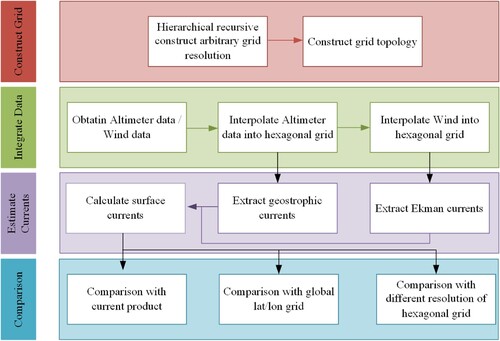
Four main steps were taken, constructing the grid, integrating data onto the grid, estimating currents using the Lagerloef ocean current algorithm, and comparison of results, as shown in Figure 1. Gridded satellite altimeter data and wind data of different resolutions were interpolated and then aggregated to the hexagonal grid based on grid cell centre. These data were used to extract both geostrophic and Ekman components for surface currents. Results were compared to three experiments.

Figure 1. Technical routine.

2.2. Construct spherical hexagonal discrete grids

The first characteristic of a grid system is what base solid it uses to represent the spheroid. Global hexagonal grids are mainly based on either an octahedron (Bai 2011) or icosahedron (Zhang et al. 2006; Bai, Zhao, and Chen 2005). We chose the icosahedron as these grids have less distortion and more uniform geometric properties.

The second characteristic of a hexagonal grid is the system used to create hierarchical recursive subdivisions. In this paper, we use Icosahedral Snyder Equal Area (ISEA) projection and pole orientation to generate a geodesic grid system (Sahr 2011). Using aperture 4 for subdivisions; that is, the area of any upper level of grid cells is four times that of the next lower level. Figure 2 shows levels 5 through 8 of our grid generated by DGGRID (Sahr 2015). Table 1 provides the number of cells and comparable coordinate based resolutions for these four levels. However, we cannot use array indices directly unless a dedicated hexagon grid index system is available (Sahr 2019). Therefore, we use half-edge structure to construct the grid geometric topology (Mcguire 2000).

Figure 2. Spherical hexagonal discrete global based on an icosahedron.

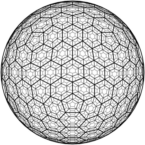
Table 1. Resolution information of the hexagonal grid.

Level	5	6	7	8
Resolution	1.96° × 1.96°	0.98° × 0.98°	0.49° × 0.49°	0.25° × 0.25°
Cells number	10242	40962	163842	655362

2.3. Integrate satellite remote sensing data on a spherical hexagonal grid

Data types from remote sensing sources included discrete points, Triangular Irregular Networks (TIN), and raster grid data. Values from TIN / rectangular grids are regarded as discrete values and are treated as discrete points at the grid centre when attributing them to the hexagonal grid. Then, the integrate method based on these sampling points can be achieved to build a hexagonal grid-based TIN/ rectangular data. The detailed procedure is as follows:

• Select the appropriate grid resolution based on the resolution of the satellite altimeter data.

• Assign terrestrial cells in the satellite altimeter data to None.

• Use nearest neighbour interpolation to aggregate data points to hexagonal grid cell centres.

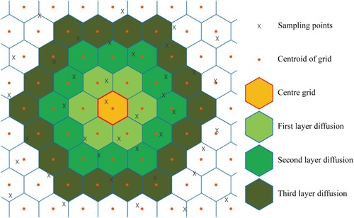
• For any hexagonal cell without an assigned value, search neighbours in recursive bands until at least four with valid values are identified (Figure 3). The cell value is estimated from the identified neighbours using the inverse distance weighted interpolation method according to the spherical distance formula (Equation 1). (1) $S=R\ast {\cos }^{-1}\left[\cos {\text{β}}_1\cos {\text{β}}_2\cos \left({\alpha }_1-{\alpha }_2\right)+\sin {\text{β}}_1\sin {\text{β}}_2\right]$(1)

The coordinates of two points on the sphere are (β₁, α₁) and (β₂, α₂), where, β is latitude and α is longitude, R is the radius of the sphere, and S is the distance.

Figure 3. Schematic diagram of diffusing query adjacent neighbour.

2.4. Extract geostrophic and Ekman components

We use spherical hexagonal grid satellite altimeter data and wind data to retrieve global ocean surface currents. According to Lagerloef et al. (1999), the ocean surface currents are the sum of the geostrophic component and Ekman component at 15 m depth, as shown in Equation (2). (2) $U=Ug+Ue$(2) where U are the surface currents, U_g ($u_g$, $v_g$) is the geostrophic component, and U_e ($u_e$, $v_e$) is the Ekman component.

2.4.1. Surface geostrophic currents

The geostrophic currents are calculated from the Absolute Dynamic Topography (ADT), which is the sum of Maps Sea Level Anomaly (MSLA) and Mean Dynamic Topographic (MDT). Therefore, ADT is the absolute dynamic topography relative to the geoid. The geostrophic balance assumes that momentum advection and frictional forces are slight. Outside the equatorial band, geostrophic velocities are given by (3a) $u_g=-{\displaystyle \frac{g}{f}\cdot {\displaystyle \frac{\mathrm{\partial }h}{\mathrm{\partial }y}}}$(3a) and (3b) $v_g=-{\displaystyle \frac{g}{f}\cdot {\displaystyle \frac{\mathrm{\partial }h}{\mathrm{\partial }x}}}$(3b) where y and x are the positions, f is the Coriolis parameter, g is the acceleration due to gravity, and h is the ADT.

Within the equatorial band, where latitude is equal to zero, the geostrophic equilibrium relationship is no longer applicable, and equatorial theory suggests using the second derivative of surface height on an equatorial β-plane. The equations for each component of the current ($u_{\text{β}},v_{\text{β}}$) on the β plane are (4a) $u_{\text{β}}=-{\displaystyle \frac{g}{\text{β}}\cdot {\displaystyle \frac{{\mathrm{\partial }}^{2}h}{\mathrm{\partial }{y}^2}}}$(4a) and (4b) $v_{\text{β}}=-{\displaystyle \frac{g}{\text{β}}\cdot {\displaystyle \frac{{\mathrm{\partial }}^{2}h}{\mathrm{\partial }x\mathrm{\partial }y}}}$(4b) where β = 2.3 * ${10}^{-11}{m}^{-1}{s}^{-1}$. Using weighting function (equation 5a and 5b) within the equatorial band to ensure the continuity of geostrophic current from the β-plane calculation in the equatorial band to the outside. Outside of this band, the estimate of the currents is still purely geostrophic. (5a) $u_g=w_f\ast u_f+w_{\text{β}}\ast u_{\text{β}}$(5a) (5b) $v_g=w_f\ast v_f+w_{\text{β}}\ast v_{\text{β}}$(5b) $w_f$ and $w_{\text{β}}$ is determined by Equation 6, where θ_S = 2.2°, C is a weighting factor. Based on the actual velocity of the currents velocity in the equatorial region, and C is set to 0.7. (6a) $w_{\text{β}}=C\ast \exp \left[-{\left({\displaystyle \frac{\theta }{{\theta }_s}}\right)}^2\right]$(6a) and (6b) $w_f=1-\exp \left[-{\left({\displaystyle \frac{\theta }{{\theta }_s}}\right)}^2\right]$(6b)

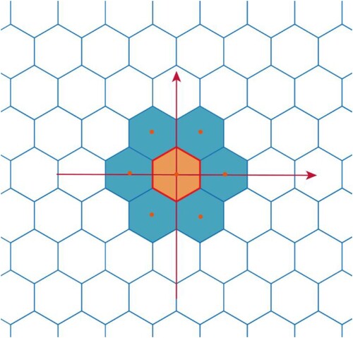
When calculating the first and second derivatives under a spherical hexagonal grid, it is necessary to orient the origin of the rectangular grid’s local plane coordinate system to the centre point of the hexagonal grid, as shown in Figure 4. The values attributed to the centre point and its surrounding six grid cells were taken as input. The first and second partial derivatives of the centre point were calculated using the bivariate quadric surface fitting, using Equation 1 to calculate the distance between centre points.

Figure 4. Orientation of local plane coordinate system for rectangular grid to the hexagonal discrete grid.

2.4.2. Surface Ekman currents

The ocean surface wind stress is the main driving force for generating Ekman currents. Thus, the ocean surface wind stress should be calculated to obtain the velocity of Ekman currents. Wind stress is a force on the ocean’s surface caused by the viscous effect of the molecules between the two layers of fluid when the wind-driven airflow moves relative to the ocean currents. The block calculation equation of the wind stress vector is: (7) $\overrightarrow{\tau }=[{\tau }_x,{\tau }_y]={\rho }_a{C}_D{V}_{10}[u_{10},u_{10}]$(7) where (τ_x, τ_y) is the wind stress field, ρ_a= 1.2 kg/${\mathrm{m}}^3$ is the air density, V₁₀ is the wind speed value at 10 m above the ocean surface, (u₁₀, v₁₀) is the wind speed value, and $C_D$ is swaying coefficient. The scheme of $C_D$ is as follows: (8) ${10}^3{C}_D=\{\begin{array}{c}0.49+0.065V_{10},V_{10}>10\mathrm{m}/\mathrm{s}\\ 1.14,3\le V_{10}\le 10\mathrm{m}/\mathrm{s}\\ 0.62+1.56V_{10}^{-1},V_{10}<3\mathrm{m}/\mathrm{s}\end{array}$(8)

For different latitudes, two sets of parameter models are used to calculate the Ekman currents:

• Within 25°S ∼ 25°N, using Equation (9). $(u_e+i{v}_e)=B{e}^{i\theta }({\tau }_x+{\tau }_y),$ (9) $\{\begin{array}{c}B={\displaystyle \frac{1}{\rho \sqrt{r^2+{\left(f{h}_{md}\right)}^2}}}\\ \theta ={\tan }^{-1}\left({\displaystyle \frac{f{h}_{md}}{r}}\right)\end{array}$(9) where ρ = 1.02 *${10}^3$kg/${\mathrm{m}}^3$is water density, r = 2.15×10⁻⁴m/s is friction coefficient, h_md = 32.5 m is mixed layer depth, f is Coriolis parameter (f = 2Ωsinφ, Ω is angular velocity of the earth’s rotation, φ is latitude), and u_e and v_e are the east and north components of the Ekman currents, respectively.

• Outside 25°S ∼ 25°N

B and θ are constants, B = 0.3ms^-1Pa^-1, θ is the turning angle relative to the wind direction, 55° to the right of the wind in the northern hemisphere and 55° to the left of the wind in the southern hemisphere.

3. Case study

The second section introduced a process to estimate ocean surface currents based on a global hexagonal grid. To evaluate the feasibility of the proposed method, we applied the process to the global ocean and analyzed the results.

3.1. Data sources

Based on the global hexagonal grid and the above method, we estimated monthly mean global ocean surface currents from satellite remote sensing data.

3.1.1. Sea surface height

The mapped Absolute Dynamic Topographic (ADT) data were processed by Data Unification and Altimeter Combination System (DUACS) and distributed by AVISO. The ADT product for the 1993-ongoing period merges altimeter measurements from five altimeter missions (Topex/Poseidon, ESR1&2, Geosat, Envisat, Jason-1). The complete DUACS process is details in (Pujol et al. 2016; Taburet et al. 2019).

3.1.2. Wind stress

The mapped monthly global wind data are averaged from daily wind fields calculated from retrievals derived from Advanced SCATterometer (ASCAT) onboard METOP-A and METOP-B satellites and distributed by Copernicus Marine Service (CMEMS). The resulting daily wind fields are estimated as equivalent neutral-stability 10 m winds. The product provides monthly mean stress-equivalent wind and stress variables as well as their standard deviation. (Copernicus 2022b).

3.1.3. Satellite currents products

We used the Global Ocean Ensemble Reanalysis data distributed by CMEMS (Copernicus 2022a) to evaluate our monthly average ocean surface currents. The ensemble comprises four reanalysis products covering the ‘altimeteric era’ period from January 1st, 1993 onward. Variables include mean temperature, salinity, currents, and ice at 1-degree horizontal resolution for 75 vertical levels.

3.1.4. Regeneration of ocean data

We used a level 6 hexagonal grid for global ocean surface currents as this level best approximates the 1° × 1° minimum resolution of source data and the lat/lon grid (Table 1). Then, we used the method introduced in section 2.3 to integrate the ocean data into the hexagonal grid and the lat/lon grid, respectively (Table 2).

Table 2. Integrated ocean data.

Data	Source resolution		Target resolution
	Temporal	Spatial	Temporal	Hexagonal Grid	Lat/Lon Grid
ADT source	Monthly mean	1/4° × 1/4°	Monthly mean	0.98 × 0.98°	1° × 1°
Wind source	Monthly mean	1/4° × 1/4°	Monthly mean	0.98 × 0.98°	1° × 1°
Currents product	Monthly mean	1° × 1°	Monthly mean	0.98 × 0.98°	1° × 1°

3.1.5. Gauge stations

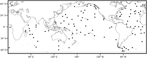
There are a total of 102 tidal gauge stations, including 22 stations in the North Atlantic, 19 stations in the South Atlantic, 18 stations in the Indian Ocean, 26 stations in the North Pacific, and 17 stations in the South Pacific. The stations are well distributed as shown in Figure 5, allowing for regional verification of our estimates. Most of these tidal gauge stations use deep-sea bottom instruments, which Shum et al. (1997) used to evaluate the accuracy of dozens of global ocean models.

Figure 5. Distribution of tidal gauge stations.

3.2. Results

3.2.1. Average ocean surface currents

Average monthly global surface currents from January 2010 to December 2019 were estimated based on satellite-derived data and the above methods. Several important global ocean circulation features can be identified in Figure 6:

1. The South (North) Equatorial Currents from east to west between 10°∼20°S (N), and the Equatorial Counter Currents flowing from west to east near the equator.

2. The Somali Currents in Indian Ocean region of the sub-plot (a).

3. The Kuroshio current flowing northward at the western border of the Pacific Ocean in the sub-plot (b).

4. The Gulf Stream flowing northward at 40°N latitude in the Atlantic Ocean in sub-plot (c).

Figure 6. The 9-year mean sea surface currents in the global oceans.

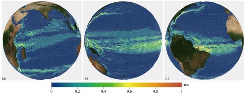
These large-scale features are consistent with both observed ocean currents and previous studies.

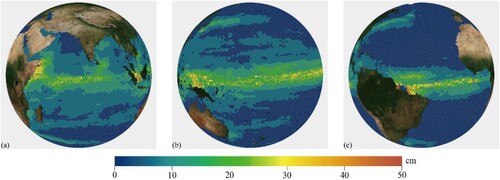
3.2.2. The standard deviation of the ocean surface currents

The standard deviation for the global ocean surface currents were computed from January 2010 to December 2019 (Figure 7). Large current variability is evident within the strong boundary currents. Throughout the equator, the standard deviation is generally above 40 cm/s, indicating that the equatorial current system is very active. In the Indian Ocean (Figure 7(a)), the most significant variation is in Somalia, where the famous Somali currents change direction with the seasons (to the south in winter and to the north in summer). This is more prominent than the Kuroshio current in the Pacific Ocean (Figure 7(b)), whose standard deviation over the 9 years is 35∼40 cm/s. In the Atlantic (Figure 7(c)), warm currents cause the Gulf of Mexico to be very active.

Figure 7. Standard deviation in global surface currents, calculated from 2010 to 2019.

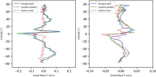
3.2.3. Zonal mean ocean surface currents

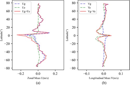
Through 9 years of inversion, the estimated zonal velocity U and meridional velocity V of the surface currents were averaged in the zonal directions, respectively, and their changes with latitude were given. In Figure 8, sub-plot (a) is the zonal profile of the zonal velocity U, where the blue dashed line represents geostrophic zonal velocity, the green dashed line represents Ekman zonal velocity, and the solid red line represents the zonal surface velocity. For the zonal velocity, the geostrophic flow caused by pressure gradient is dominant, especially in the middle and high latitudes, where the Ekman flow is much weaker than the geostrophic flow. Sub-plot (b) of Figure 8 shows the zonal profile of meridional velocity V. These figures suggest the Ekman flow caused by wind stress is dominant for meridional velocity, and the geotropic meridional flow is much weaker than the Ekman flow. Therefore, the structure of ocean flow estimated by satellite remote sensing inversion obtained in Figure 8 conforms to the basic law of earth fluid motion.

Figure 8. The zonal profile of zonal mean U and longitudinal mean V.

4. Comparisons

To verify the accuracy of ocean surface currents extracted to a global hexagonal grid, we carried out a three part experimental verification. First, we evaluated the hexagon grid-based results against the observational datasets. Second, we compared the hexagon grid-based and lat/lon grid-based results. Finally, the extraction accuracy of several different resolution grids was compared.

4.1. Comparison with current product

Several satellite near-surface current products exist and are distributed over various platforms. We selected validation data with the same resolutions as our resulting data (see section 3.1.3 for details). The U and V components of the ocean surface currents obtained by the model algorithm and those of the validated ocean currents data were averaged along the latitude for nine years. Figure 9 shows the relative U/V component error compared to the currents product. The blue line represents the calculation results under the hexagonal grid, the green line represents the currents product, and the red dashed line represents the relative error between them (unit: m/s). The U component had small overall error, with the largest error (0.1 m/s) near the equator. The V component similarly had the largest error near the equator, around 25 degrees north and south latitude.

Figure 9. U and V component error comparison.

4.2. Comparison with global lat/lon grid

This paper verifies the advantages of the hexagonal discrete grid in extracting surface currents from satellite remote sensing data by comparing the results of global surface currents with those of lat/lon grids. We use the same model and same level 6 approximate resolution (See Table 2) to extract the global surface ocean surface currents based on the global hexagonal grid and the global lat/lon grid, respectively.

Figures 10 and 11 compare the Absolute Errors (AE) in U and V components between the two types of grids to the validation data based on the mean value of 9 years’ monthly mean flow obtained by inversion. In the Figures, subplot a ∼ c and g ∼ i show AE under the global hexagonal grids, and subplot d ∼ f and j ∼ l show AE under the global lat/lon grids. The error units are m/s.

Figure 10. Absolute Error comparison of U component based of two type of grids.

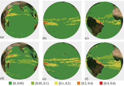
Figure 11. Absolute Error comparison of V component based of two type of grids.

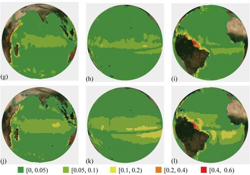
From the figures, it can be concluded that:

1. The AE of U/V components are less than 0.05 m/s for both types of grids in ocean areas with gentle velocities.

2. The error is greater in near-shore areas and where ocean currents are stronger, with a maximum of over 0.4 m/s.

3. For the U component velocity, the calculation errors based on the global lat/lon grid in the south/north equatorial current and equatorial countercurrent are larger than those under the global hexagonal grid.

4. For the V component velocity, the calculation error in the global hexagon is mainly distributed in the range of 0.05 ∼ 0.1 m/s. Although the calculation error in the lat/lon grid cells is mainly in the same range, far more cells have 0.1 ∼ 0.2 m/s error.

Table 3 compares the result accuracy of the two types of grids by quantifying the proportion of grid cell in each category from Figures 10 and 11. The proportion of hexagonal grid cells in the [0, 0.05] category is about 2% greater than that of the lat/lon grid, for both the U and V components, indicating the hexagonal grid more often calculates currents with errors under 0.05 m/s. Within the error range of [0.05∼0.2], the proportion of hexagonal grid cells in U and V components is 10.18% and 13.32%, respectively, while the proportion of lat/lon grid cells is 13.54% and 15.28%, respectively. Although the proportion of hexagonal grid cells is slightly greater than that of lat/lon grid cells in the [0.2 ∼0.6] error interval, these cells represent less than 1%, a limited proportion. Therefore, it is reasonable to conclude that the hexagonal grid has higher accuracy than the global lat/lon grid when calculating ocean currents from satellite data.

Table 3. Percent of grid cells of each category.

Category (m/s)	AE of U component (%)		AE of V component (%)
	Hexagon	Lat/Lon	Hexagon	Lat/Lon
[0, 0.05]	88.94	85.49	86.09	84.36
[0.05, 0.1]	7.34	9.77	11.07	11.87
[0.1, 0.2]	2.84	3.77	2.25	3.41
[0.2, 0.4]	0.8	0.92	0.54	0.33
[0.4, 0.6]	0.08	0.04	0.05	0.03

4.3. Comparison of different resolution of hexagonal grids

A global hexagonal grid with level 6 resolution corresponds to a spatial resolution of 1 degree. However, the influence of grid resolution on surface ocean current extraction is also an important part of the experiment. Therefore, we compare the extraction accuracy of several different resolutions of hexagonal grids.

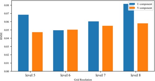
In this section, we evaluated four levels of hexagonal grid (level 5 ∼ level 8, as shown in Table 1) on their ability to estimate monthly mean ocean currents for 2019 compared to gauge stations (Figure 5). Using the hexagonal grid estimates, we interpolate the value at each tide gauge station for comparison. Error (RMSE) is calculated at 102 points where tide gauge data was available, but five of the points were omitted because they were on small islands. Figure 12 shows the level 6 grid had the smallest overall error (see Appendix 1–2 for specific data).

Figure 12. RMSE of estimates from different level grids when compared to gauge stations.

5. Discussions

5.1. The advantages of an isotropic hexagonal grid

Figures 10 and 11 show the U component flow error is larger than that of the V component flow, likely because mainly geostrophic currents control the U component flow. Calculating geostrophic currents requires interpolating elevation points and calculating first and second-order gradients by surface fitting. As a result, the U component is more error prone and less accurate than the V component.

The same figures show when grid resolution is the same, the error of estimated based on the isotropic hexagon is smaller than that of estimates based on the global lat/lon grid. Huang (2018) concluded that the uniform distribution of control points improves of the accuracy of interpolation results. Therefore, the more uniform distribution of cells in a discrete hexagonal grid improves the accuracy of geostrophic elevation plane interpolation fitting compared to a lat/lon grid.

5.2. The optimal hexagonal grid resolution

With 1°×1° monthly average ocean current product data as comparative data, we compared the extraction accuracy under different grid resolutions in section 4.3. As shown in Figure 12, the greatest extraction accuracy was achieved for both U and V components when using a level 6 grid. We find that the resolution of the grid affects the accuracy of the extraction results, and it is not that the higher the grid resolution, the higher the accuracy of the extracted currents. This conclusion is in line with the findings of Hodgson (1995) and Kenward et al. (2000) that terrain data quality and resolution significantly affect the accuracy of any extracted hydrological features. Vaze, Teng, and Spencer (2010) concluded that terrain process scale is the key driver in determining useful grid resolution cell.

There are significant differences in extraction results based on high resolution and coarse resolutions of the hexagonal grid. However, as a limitation of this study, we did not study in depth the effect of hexagonal grid cell size on ocean currents information extracted from satellite data. Meanwhile, global lat/lon grids are not true rectangular grids (poles) and grid cells are far from equal area. When comparing with the extraction results of hexagon grid with the same resolution, this will cause some errors in the analysis of the results. Therefore, we will deeply explore this question in future research.

6. Conclusions

Global lat/lon grids have inherent differences in distance measurements across eight directions due to the isotropy, thus inhibiting the extraction of global surface currents to such grids. However, in the tessellation model representing real planar space, the hexagon, as a regular grid, has superior performance due to its consistent connectivity, compact structure, and isotropic local neighbourhood. Therefore, a method of global surface ocean currents based on global hexagonal grid is proposed in this paper. The effectiveness of the proposed method is tested by applying it to 9 years of monthly average ocean satellite remote sensing data. Compared with the method based on global lat/lon grid at the same resolution, the following conclusions can be drawn:

1. The global hexagonal grid provides a framework for processing global ocean satellite remote sensing data. The extraction results for nine years’ monthly mean ocean flow are consistent with the law of ocean surface currents and compared with the validation data.

2. Results calculated based on the hexagonal grid compared favourably to those calculated based on a lat/lon grid of the same resolution. based on the greater accuracy relative to validation data it can be concluded that the isotropic grid has advantages over the lat/lon grid when processing satellite data.

3. This paper demonstrates the important influence of grid geometry on estimates of global surface ocean currents and provides a new approach for the spatial analysis of ocean data.

Data and availability statement

The data that support the findings of this study are available through the following private link: https://doi.org/10.5281/zenodo.7588392.

Disclosure statement

No potential conflict of interest was reported by the author(s).

Additional information

Funding

This work was supported by the National Nature Science Foundation of China [42076203].

Appendices

Appendix 1

Table

Numerical comparison u component
num_index	lat	lon	Valid	Level5	Level6	Level7	Level8
1	60.2	−28.8	−0.0041	−0.0039	−0.0042	−0.0165	−0.0355
2	57.2	−10.1	0.0122	0.0225	0.0246	0.0155	0.0158
3	54	−52.8	0.0279	0.0325	0.0675	0.0397	0.0411
4	53.6	−13.9	0.0206	0.0199	0.0154	0.0086	0.0087
5	53.5	−25.1	0.0250	0.0308	0.0262	0.0282	0.0494
6	44.5	−40.5	0.0690	0.0701	0.0468	−0.0388	−0.0687
7	41.4	−28	0.0340	0.0265	0.0419	0.0578	0.0714
8	40.3	−15	0.0021	0.0091	0.0108	0.0120	0.0112
9	39.5	−31.1	0.0208	0.0234	0.0245	0.0100	0.0034
10	37.8	−68	0.4101	0.1450	0.3750	0.6572	0.8472
11	37.2	−20.1	−0.0008	0.0123	0.0042	0.0079	0.0099
12	34	−29.4	0.0413	0.0181	0.0452	0.0508	0.0668
13	33.9	−41.2	0.0436	0.0199	0.0466	0.0673	0.0757
15	32.4	−64.7	−0.0209	−0.0109	−0.0289	−0.0397	−0.0497
16	28.5	−76.8	−0.0171	0.0353	−0.0227	−0.0165	−0.0083
17	28.2	−67.5	0.0218	0.0001	0.0209	0.0373	0.0420
18	26.6	−44	0.0057	−0.0069	0.0017	0.0116	0.0193
19	26.5	−69.3	−0.0016	0.0069	0.0066	−0.0012	0.0003
20	24.8	−89.6	−0.0436	0.0189	−0.0154	−0.0416	−0.0503
21	14.9	−23.5	−0.0373	0.0222	0.0248	0.0292	0.0550
22	14.7	−48.8	−0.0198	−0.0219	−0.0093	−0.0073	−0.0042
23	7	−51.5	−0.0711	0.0375	−0.0438	−0.1378	−0.2197
24	0.9	−29.3	−0.1420	−0.0694	−0.1066	−0.1274	−0.0934
25	0.2	−41.2	−0.2967	−0.0985	−0.2039	−0.1813	−0.1228
26	0	−20	−0.1197	−0.0913	−0.1204	−0.1200	−0.2178
27	0	−10	−0.1119	−0.0633	−0.1983	−0.2153	−0.2802
28	−1.4	5.6	−0.0748	0.0522	0.0351	0.0387	0.0048
29	−3.8	−32.4	−0.2010	−0.1163	−0.1448	−0.1297	−0.1291
30	−7.9	−14.4	−0.0678	0.0179	0.0365	0.0177	0.0045
31	−15.9	−5.7	−0.0589	−0.0265	−0.0354	−0.0318	−0.0250
32	−17.1	−13.7	−0.0613	−0.0379	−0.0472	−0.0498	−0.0499
33	−18	−36.1	−0.0007	−0.0235	−0.0114	−0.0220	−0.0292
34	−20.5	−29.3	−0.0146	−0.0157	−0.0215	−0.0242	−0.0252
35	−38.5	−11.1	0.0359	0.0452	0.0319	0.0133	−0.0022
36	−53.5	−57	0.0455	0.0932	0.0487	0.0020	−0.0001
38	−54.5	3.3	0.0394	0.0816	0.0714	0.0544	0.0462
39	−56.5	−63	0.0891	0.1285	0.1236	0.0539	0.0380
40	−56.7	−52.5	0.1565	0.0948	0.1470	0.1546	0.1858
41	−60	−47.1	0.0404	0.0539	0.0266	0.0290	0.0099
42	−61.5	−61.3	0.0545	0.0924	0.0390	0.0966	0.1066
43	4.2	52.9	−0.0563	−0.0277	−0.1167	−0.1316	−0.1384
44	4.2	73.5	−0.0336	−0.0207	−0.0305	−0.0211	−0.0167
45	−0.7	73.2	−0.1387	−0.0223	−0.0681	−0.0893	−0.0825
46	−4.6	55.5	0.0571	0.1004	0.1293	0.1044	0.0977
47	−9.4	46.2	−0.2630	−0.1410	−0.3375	−0.4182	−0.4390
48	−10.4	105.7	−0.2473	−0.0843	−0.1603	−0.1895	−0.1939
49	−10.4	56.7	−0.1470	−0.0663	−0.0790	−0.0692	−0.0615
50	−12.1	96.9	−0.0964	−0.0421	−0.0346	−0.0304	−0.0262
51	−12.8	45.3	−0.1578	−0.1275	−0.0086	0.0413	0.0876
52	−19.7	63.4	−0.0171	−0.0166	−0.0078	0.0036	0.0066
53	−20.2	57.5	−0.0217	−0.0142	−0.0166	−0.0040	−0.0238
54	−28.3	66.8	0.0001	0.0306	0.0101	0.0008	−0.0018
55	−37	132	0.0005	0.0041	0.0047	−0.0014	−0.0056
56	−37.9	77.6	0.0262	0.0234	0.0226	0.0194	0.0172
57	−50	132.1	0.1156	0.1213	0.1517	0.1816	0.1927
58	−53	73.4	0.0138	0.0625	0.0309	0.0299	0.0229
59	−60	132.1	0.0578	0.0627	0.0639	0.0723	0.0669
60	59.1	−175.1	−0.0162	0.0034	−0.0117	−0.0032	0.0036
61	56.1	−144.4	0.0050	−0.0090	−0.0122	−0.0200	−0.0244
62	53.4	−154.3	0.0033	−0.0090	−0.0193	−0.0217	−0.0190
63	53.3	−135.6	0.0126	0.0035	0.0065	0.0143	0.0190
65	49.6	−132.8	0.0030	0.0116	0.0093	0.0081	0.0061
66	46.8	−130.8	0.0137	0.0119	0.0191	0.0184	0.0169
67	43.3	−160.1	0.0388	0.0393	0.0369	0.0448	0.0493
68	40.7	−169.4	0.0407	0.0496	0.0464	0.0335	0.0328
69	36.5	−164	0.0383	0.0356	0.0367	0.0336	0.0298
70	33.5	−134.2	0.0092	0.0038	0.0096	0.0152	0.0097
71	32	149.8	−0.0508	0.0439	−0.0241	−0.0100	−0.0081
72	28.2	−177.4	0.0197	0.0191	0.0253	0.0379	0.0405
73	27.1	142.2	0.0187	−0.0081	0.0142	0.0109	0.0084
74	25	−133.9	0.0100	0.0160	0.0155	0.0220	0.0281
75	24.3	154	0.0461	0.0123	0.0311	0.0176	0.0221
76	23.9	−166.3	0.0045	0.0098	0.0156	0.0294	0.0362
77	21.5	−109.9	0.0145	0.0379	0.0369	0.0455	0.0487
78	19.3	166.6	−0.0010	−0.0348	−0.0140	−0.0053	−0.0071
79	18.9	−152.5	−0.0588	−0.0445	−0.0570	−0.0550	−0.0515
80	18.7	−111	0.0095	0.0402	0.0405	0.0297	0.0208
81	16.7	−169.5	−0.0692	−0.0450	−0.0379	−0.0460	−0.0493
82	15.2	145.7	−0.0883	−0.0964	−0.0840	−0.0767	−0.0705
83	9.5	138.1	−0.1359	−0.0842	−0.1407	−0.1354	−0.1287
84	7.1	171.4	0.1074	0.1134	0.1557	0.1420	0.1459
85	7	158.2	0.0792	0.0848	0.1103	0.1110	0.0540
87	1.4	172.9	−0.2042	0.0367	0.0118	0.0461	0.0960
88	−0.4	−90.3	−0.2211	−0.1966	−0.3021	−0.3232	−0.3443
89	−2	147.3	−0.1241	0.1915	0.0779	−0.0042	0.0664
90	−2.9	−95	−0.2180	−0.1171	−0.0892	−0.0995	−0.1253
91	−8.5	179.2	0.0269	−0.0293	0.0014	0.0268	0.0369
92	−8.9	−140.1	−0.0931	−0.1022	−0.0834	−0.0595	−0.0705
93	−14.3	−170.7	−0.0066	−0.0249	−0.0089	−0.0061	0.0072
95	−17.8	168.3	−0.0110	0.0170	0.0295	0.0393	0.0406
96	−21.2	−159.8	0.0171	0.0219	0.0167	0.0250	0.0430
97	−23.1	−134.9	0.0141	0.0170	0.0112	0.0196	0.0224
98	−27.2	−109.4	0.0099	0.0081	0.0024	−0.0013	−0.0023
99	−29.1	167.9	0.0055	0.0256	0.0053	0.0092	0.0149
100	−31.5	159.1	0.0117	0.0331	0.0035	0.0115	0.0138
101	−33.6	−78.8	−0.0049	0.0008	−0.0016	−0.0054	0.0000
102	−54.5	159	0.2014	0.1405	0.1659	0.1423	0.1219

Appendix 2

Table

Numerical comparison v component
num_index	lat	lon	Valid	Level5	Level6	Level7	Level8
1	60.2	−28.8	0.0422	0.0122	0.0165	0.0122	−0.0090
2	57.2	−10.1	0.0069	0.0107	0.0106	0.0192	0.0179
3	54	−52.8	−0.1125	0.0009	−0.0523	−0.1647	−0.1917
4	53.6	−13.9	0.0149	0.0101	0.0125	0.0291	0.0263
5	53.5	−25.1	−0.0027	0.0136	0.0207	0.0059	−0.0098
6	44.5	−40.5	0.0049	0.0118	0.0213	0.0476	0.0535
7	41.4	−28.0	−0.0167	0.0037	0.0002	0.0054	0.0000
8	40.3	−15.0	−0.0160	0.0026	−0.0086	−0.0182	−0.0187
9	39.5	−31.1	−0.0269	0.0023	−0.0085	−0.0221	−0.0281
10	37.8	−68.0	0.0136	0.0160	0.0344	0.1054	0.1352
11	37.2	−20.1	−0.0130	0.0028	−0.0071	−0.0159	−0.0163
12	34	−29.4	−0.0104	0.0040	−0.0047	−0.0254	−0.0370
13	33.9	−41.2	−0.0385	−0.0014	−0.0191	−0.0421	−0.0587
15	32.4	−64.7	−0.0211	0.0020	−0.0098	−0.0290	−0.0352
16	28.5	−76.8	0.0221	0.0159	0.0195	−0.0037	−0.0090
17	28.2	−67.5	−0.0009	0.0015	0.0042	0.0028	0.0006
18	26.6	−44.0	0.0125	0.0041	0.0009	0.0027	0.0051
19	26.5	−69.3	0.0114	0.0028	0.0027	0.0038	0.0023
20	24.8	−89.6	0.0344	0.0147	0.0346	0.0131	0.0022
21	14.9	−23.5	−0.0017	−0.0006	−0.0120	−0.0398	−0.0440
22	14.7	−48.8	0.0317	−0.0147	−0.0362	−0.0576	−0.0611
23	7	−51.5	0.2206	−0.0142	−0.0025	0.0487	0.0683
24	0.9	−29.3	0.0275	0.0093	−0.0075	−0.0296	−0.0452
25	0.2	−41.2	0.0177	−0.0005	0.0183	0.0577	0.0626
26	0	−20.0	−0.0176	0.0227	0.0297	0.0381	0.0334
27	0	−10.0	−0.0389	0.0177	0.0137	0.0074	−0.0137
28	−1.4	5.6	−0.0401	0.0188	0.0333	0.0163	0.0506
29	−3.8	−32.4	−0.0613	0.0388	0.0983	0.1196	0.1160
30	−7.9	−14.4	−0.0447	0.0521	0.0773	0.1241	0.1260
31	−15.9	−5.7	−0.0089	0.0233	0.0341	0.0422	0.0436
32	−17.1	−13.7	−0.0146	0.0201	0.0235	0.0271	0.0273
33	−18	−36.1	−0.0410	0.0117	−0.0068	−0.0155	−0.0092
34	−20.5	−29.3	−0.0049	0.0111	0.0072	0.0040	0.0048
35	−38.5	−11.1	0.0328	0.0143	0.0170	0.0329	0.0344
36	−53.5	−57.0	0.1014	0.0261	0.0502	0.0744	0.0566
38	−54.5	3.3	0.0281	0.0170	0.0196	0.0283	0.0183
39	−56.5	−63.0	0.0860	0.0264	0.0643	0.1060	0.1128
40	−56.7	−52.5	0.0347	0.0290	0.0543	0.0325	−0.0131
41	−60	−47.1	0.0026	0.0194	0.0145	−0.0054	−0.0103
42	−61.5	−61.3	0.0569	0.0269	0.0414	0.0734	0.0897
43	4.2	52.9	0.0280	0.0334	0.0730	0.0998	0.1174
44	4.2	73.5	−0.0167	0.0115	0.0005	0.0006	0.0025
45	−0.7	73.2	−0.0207	0.0106	0.0095	0.0224	0.0361
46	−4.6	55.5	−0.0264	0.0122	0.0194	0.0260	0.0262
47	−9.4	46.2	0.0502	0.0395	0.0791	0.1030	0.1149
48	−10.4	105.7	−0.0317	0.0329	0.0687	0.0911	0.0930
49	−10.4	56.7	−0.0801	0.0216	0.0215	0.0230	0.0232
50	−12.1	96.9	−0.0500	0.0304	0.0501	0.0639	0.0651
51	−12.8	45.3	0.0224	0.0249	0.0239	0.0361	0.0272
52	−19.7	63.4	−0.0327	0.0136	0.0133	0.0087	0.0053
53	−20.2	57.5	−0.0361	0.0123	0.0044	−0.0039	−0.0075
54	−28.3	66.8	0.0002	0.0135	0.0137	0.0165	0.0165
55	−37	132.0	0.0189	0.0077	0.0086	0.0076	0.0046
56	−37.9	77.6	0.0311	0.0154	0.0168	0.0146	0.0147
57	−50	132.1	0.0333	0.0101	0.0290	0.0504	0.0664
58	−53	73.4	0.0434	0.0190	0.0257	0.0248	0.0138
59	−60	132.1	−0.0187	0.0043	−0.0013	0.0020	−0.0009
60	59.1	−175.1	0.0180	0.0099	0.0150	0.0171	0.0173
61	56.1	−144.4	0.0151	0.0080	0.0150	0.0237	0.0220
62	53.4	−154.3	0.0012	0.0043	0.0036	0.0234	0.0289
63	53.3	−135.6	0.0063	0.0068	0.0079	0.0018	−0.0044
65	49.6	−132.8	−0.0085	0.0049	0.0021	−0.0019	−0.0038
66	46.8	−130.8	−0.0039	0.0022	0.0003	0.0000	0.0009
67	43.3	−160.1	−0.0090	0.0058	0.0022	−0.0032	−0.0046
68	40.7	−169.4	−0.0067	0.0051	0.0032	0.0001	0.0031
69	36.5	−164.0	−0.0083	0.0037	0.0023	−0.0060	−0.0114
70	33.5	−134.2	−0.0147	0.0004	−0.0073	−0.0205	−0.0240
71	32	149.8	−0.0182	−0.0024	−0.0186	−0.0503	−0.0573
72	28.2	−177.4	−0.0035	0.0057	0.0015	−0.0087	−0.0072
73	27.1	142.2	−0.0159	0.0018	−0.0103	−0.0345	−0.0417
74	25	−133.9	0.0052	0.0026	−0.0011	−0.0021	−0.0003
75	24.3	154.0	0.0066	0.0008	−0.0019	−0.0015	0.0011
76	23.9	−166.3	0.0134	0.0047	0.0005	−0.0025	−0.0032
77	21.5	−109.9	−0.0144	0.0039	0.0001	−0.0021	0.0093
78	19.3	166.6	0.0130	−0.0042	−0.0133	−0.0270	−0.0319
79	18.9	−152.5	0.0432	0.0059	0.0175	0.0213	0.0232
80	18.7	−111.0	−0.0092	0.0028	−0.0045	−0.0085	−0.0116
81	16.7	−169.5	0.0225	−0.0013	−0.0122	−0.0275	−0.0319
82	15.2	145.7	0.0359	−0.0019	−0.0138	−0.0314	−0.0370
83	9.5	138.1	0.0599	0.0062	0.0004	−0.0171	−0.0216
84	7.1	171.4	0.0492	−0.0214	−0.0583	−0.0779	−0.0775
85	7	158.2	0.0563	−0.0085	−0.0245	−0.0282	−0.0224
87	1.4	172.9	0.0392	−0.0073	−0.0215	−0.0326	−0.0385
88	−0.4	−90.3	−0.0076	0.0095	0.0096	−0.0749	−0.1083
89	−2	147.3	−0.0432	0.0028	0.0202	0.0372	0.0273
90	−2.9	−95.0	−0.1175	0.0240	0.0375	0.0234	0.0197
91	−8.5	179.2	−0.0141	0.0009	0.0064	0.0040	0.0018
92	−8.9	−140.1	−0.0300	0.0407	0.0667	0.0935	0.0969
93	−14.3	−170.7	−0.0237	0.0096	0.0206	0.0260	0.0243
95	−17.8	168.3	−0.0591	0.0020	−0.0009	0.0015	−0.0083
96	−21.2	−159.8	−0.0226	0.0054	0.0052	0.0115	0.0186
97	−23.1	−134.9	−0.0171	0.0055	0.0014	−0.0062	−0.0046
98	−27.2	−109.4	−0.0027	0.0080	0.0059	0.0007	0.0001
99	−29.1	167.9	0.0016	0.0042	0.0044	0.0077	0.0144
100	−31.5	159.1	0.0347	0.0083	0.0265	0.0324	0.0253
101	−33.6	−78.8	0.0142	0.0171	0.0241	0.0354	0.0312
102	−54.5	159.0	0.1023	−0.0024	0.0271	0.0912	0.1226

References

- An, Yuzhu, Ren Zhang, Huizan Wang, Jian Chen, and Weitao Zhang. 2012. “Ocean Surface Currents Retrieval Based on Satellite Remote Sensing Data.” Marine Science Bulletin 31 (1): 1–8. doi:10.3969/j.issn.1001-6392.2012.01.001.
- Bai, Jianjun. 2011. “Location Coding and Indexing Aperture 4 Hexagonal Discrete Global Grid Based on Octahedron.” Journal of Remote Sensing 15 (6): 1125–37. doi:10.11834/jrs.20110367.
- Bai, Jianjun, Xuesheng Zhao, and Jun Chen. 2005. “Indexing of Discrete Global Grids Using Linear Quadtree.” Geomatics and Information Science of Wuhan University 30 (9): 805–8. doi:10.3969/j.issn.1671-8860.2005.09.013.
- Baumann, Peter. 2021. “A General Conceptual Framework for Multi-Dimensional Spatio-Temporal Data Sets.” Environmental Modelling & Software 143: 105096. doi:10.1016/j.envsoft.2021.105096.
- Birch, Colin P. D., Sander P. Oom, and Jonathan A. Beecham. 2007. “Rectangular and Hexagonal Grids Used for Observation, Experiment and Simulation in Ecology.” Ecological Modelling 206 (3-4): 347–59. doi:10.1016/j.ecolmodel.2007.03.041.
- Chelton, Dudley B., Michael G. Schlax, and Roger M. Samelson. 2011. “Global Observations of Nonlinear Mesoscale Eddies.” Progress in Oceanography 91 (2): 167–216. doi:10.1016/j.pocean.2011.01.002
- Copernicus. 2022a. Global Ocean Ensemble Physics Reanalysis – Low Resolution. Copernicus Marine Service. Accessed 9 September 2022. doi:10.48670/moi-00181.
- Copernicus. 2022b. Global Ocean Monthly Mean Sea Surface Wind and Stress from Scatterometer and Model. Copernicus Marine Service. Accessed 12 September 2022. doi:10.48670/moi-00181.
- García Molinos, J., M. T. Burrows, and Elvira S. Poloczanska. 2017. “Ocean Currents Modify the Coupling Between Climate Change and Biogeographical Shifts.” Scientific Reports 7 (1): 1332. doi:10.1038/s41598-017-01309-y.
- Girard, Charlotte, Joël Sudre, Simon Benhamou, David Roos, and Paolo Luschi. 2006. “Homing in Green Turtles Chelonia Mydas: Oceanic Currents Act as a Constraint Rather Than as an Information Source.” Marine Ecology Progress Series 322: 281–9. doi:10.3354/meps322281
- Han, Bing, Tengteng Qu, Zili Huang, Qiangyu Wang, and Xinlong Pan. 2022. “Emergency Airport Site Selection Using Global Subdivision Grids.” Big Earth Data 6 (3): 276–93. doi:10.1080/20964471.2021.1996866.
- Hodgson, Michael E. 1995. “What Cell Size Does the Computed Slope/Aspect Angle Represent.” Photogrammetric Engineering and Remote Sensing 6 (5): 513–7.
- Hojati, Majid, Colin Robertson, Steven Roberts, and Chiranjib Chaudhuri. 2022. “GIScience Research Challenges for Realizing Discrete Global Grid Systems as a Digital Earth.” Big Earth Data 6 (3): 358–79. doi:10.1080/20964471.2021.2012912.
- Huang, Zhongde. 2018. “Study on the Accuracy of Gps Elevation Fitting Model for Quadric Surface.” Western Resources 5: 144–5. doi:10.16631/j.cnki.cn15-1331/p.2018.05.154.
- Kenward, Tracey, Dennis P. Lettenmaier, Eric F. Wood, and Eric Fielding. 2000. “Effects of Digital Elevation Model Accuracy on Hydrologic Predictions.” Remote Sensing of Environment 74 (3): 432–44. doi:10.1016/S0034-4257(00)00136-X.
- Kimerling, Jon A., Kevin Sahr, Denis White, and Lian Song. 1999. “Comparing Geometrical Properties of Global Grids.” Cartography and Geographic Information Science 26 (4): 271–88. doi:10.1559/152304099782294186.
- Kmoch, Alexander, Ivan Vasilyev, Holger Virro, and Evelyn Uuemaa. 2022. “Area and Shape Distortions in Open-Source Discrete Global Grid Systems.” Big Earth Data 6 (3): 256–75. doi:10.1080/20964471.2022.2094926.
- Lagerloef, Gary S. E., Roger Lukas, Fabrice Bonjean, John T. Gunn, Gary T. Mitchum, Mark Bourassa, and Antonio J. Busalacchi. 2003. “El Niño Tropical Pacific Ocean Surface Current and Temperature Evolution in 2002 and Outlook for Early 2003.” Geophysical Research Letters 30 (10): 1514. doi:10.1029/2003GL017096.
- Lagerloef, Gary Se, Gary T Mitchum, Roger B Lukas, and Pearn P Niiler. 1999. “Tropical Pacific Near-Surface Currents Estimated from Altimeter, Wind, and Drifter Data.” Journal of Geophysical Research: Oceans 104 (C10): 23313–26. doi:10.1029/1999JC900197
- Lai, Guangling, Xiaochong Tong, Yong Zhang, Lu Ding, Kai Li, and Shuaibo Fan. 2016. “Research on the Method of Urban Waterlogging Flood Routing Based on Hexagonal Grid.” Acta Geodaetica et Cartographica Sinica 45 (S1): 144–51. doi:10.11947/j.AGCS.2016.F018.
- Liao, Chang, Teklu Tesfa, Zhuoran Duan, and L. Ruby Leung. 2020. “Watershed Delineation on a Hexagonal Mesh Grid.” Environmental Modelling & Software 128: 104702. doi:10.1016/j.envsoft.2020.104702.
- Liu, Wei, Ren Zhang, Huizan Wang, Yuzhu An, and Zhisong Huang. 2012. “Sea Surface Flow Field Retrieval and Estimation Based on Satellite Remote Sensing Data.” Progress in Geophysics 27 (5): 1989–94. doi:10.6038/j.issn.1004-2903.2012.05.020.
- Llido, J., V. Garçon, J. R. E. Lutjeharms, and J. Sudre. 2005. “Event-Scale Blooms Drive Enhanced Primary Productivity at the Subtropical Convergence.” Geophysical Research Letters 32 (15): L15611. doi:10.1029/2005GL022880.
- Maes, Christophe, Kentaro Ando, Thierry Delcroix, William S. Kessler, Michael J. Mcphaden, and Dean Roemmich. 2006. “Observed Correlation of Surface Salinity, Temperature and Barrier Layer at the Eastern Edge of the Western Pacific Warm Pool.” Geophysical Research Letters 33 (6): L06601. doi:10.1029/2005GL024772.
- Maes, Christophe, Joël Sudre, and Véronique Garçon. 2010. “Detection of the Eastern Edge of the Equatorial Pacific Warm Pool Using Satellite-Based Ocean Color Observations.” Sola 6: 129–32. doi:10.2151/sola.2010-033
- Mahdavi-Amiri, Ali, Erika Harrison, and Faramarz Samavati. 2015. “Hexagonal Connectivity Maps for Digital Earth.” International Journal of Digital Earth 8 (9): 750–69. doi:10.1080/17538947.2014.927597
- Mcguire, Max. 2000. “The Half-Edge Data Structure.” Website. http://www.flipcode.com/articles/article.halfedgepf.shtml.
- Middleton, Lee, and Jayanthi Sivaswamy. 2005. Hexagonal Image Processing: A Practical Approach. London: Springer-Verlag.
- Picaut, J., M. Ioualalen, C. Menkès, T. Delcroix, and M. J. Mcphaden. 1996. “Mechanism of the Zonal Displacements of the Pacific Warm Pool: Implications for ENSO.” Science 274 (5292): 1486–9. doi:10.1126/science.274.5292.1486.
- Poloczanska, Elvira S., Michael T. Burrows, Christopher J. Brown, Jorge García Molinos, Benjamin S. Halpern, Ove Hoegh-Guldberg, Carrie V. Kappel, et al. 2016. “Responses of Marine Organisms to Climate Change Across Oceans.” Frontiers in Marine Science 3: 62. doi:10.3389/fmars.2016.00062.
- Pujol, M. I., Y. Faugère, G. Taburet, S. Dupuy, C. Pelloquin, M. Ablain, and N. Picot. 2016. “Duacs DT2014: The New Multi-Mission Altimeter Data Set Reprocessed Over 20 Years.” Ocean Science 12 (5): 1067–90. doi:10.5194/os-12-1067-2016.
- Rawson, Andrew, Zoheir Sabeur, and Mario Brito. 2022. “Intelligent Geospatial Maritime Risk Analytics Using the Discrete Global Grid System.” Big Earth Data 6 (3): 294–322. doi:10.1080/20964471.2021.1965370.
- Sahr, Kevin. 2011. “Hexagonal Discrete Global Grid Systems for Geospatial Computing.” Archiwum Fotogrametrii, Kartografii i Teledetekcji 22: 363–76.
- Sahr, Kevin. 2015. DGGRID Version 6.2 B: User Documentation for Discrete Global Grid Generation Software. Southern Oregon University, September 20. https://webpages.sou.edu/~sahrk/sqspc/pubs/dggridManualV62.pdf.
- Sahr, Kevin. 2019. “Central Place Indexing: Hierarchical Linear Indexing Systems for Mixed-Aperture Hexagonal Discrete Global Grid Systems.” Cartographica: The International Journal for Geographic Information and Geovisualization 54 (1): 16–29. doi:10.3138/cart.54.1.2018-0022.
- Shum, C. K., P. L. Woodworth, O. B. Andersen, Gary D. Egbert, O. Francis, C. King, S. M. Klosko, et al. 1997. “Accuracy Assessment of Recent Ocean Tide Models.” Journal of Geophysical Research: Oceans 102 (C11): 25173–94. doi:10.1029/97JC00445.
- Sudre, Joel, Christophe Maes, and Veronique Garçon. 2013. “On the Global Estimates of Geostrophic and Ekman Surface Currents.” Limnology and Oceanography: Fluids and Environments 3 (1): 1–20. doi:10.1215/21573689-2071927
- Sudre, Joel, and Rosemary A. Morrow. 2008. “Global Surface Currents: A High-Resolution Product for Investigating Ocean Dynamics.” Ocean Dynamics 58 (2): 101–18. doi:10.1007/s10236-008-0134-9.
- Taburet, G., A. Sanchez-Roman, M. Ballarotta, M. I. Pujol, J. F. Legeais, F. Fournier, Y. Faugere, and G. Dibarboure. 2019. “Duacs dt2018: 25 Years of Reprocessed Sea Level Altimetry Products.” Ocean Science 15 (5): 1207–24. doi:10.5194/os-15-1207-2019.
- Tai, Chang-Kou. 1988. “Geosat Crossover Analysis in the Tropical Pacific: 1. Constrained Sinusoidal Crossover Adjustment.” Journal of Geophysical Research: Oceans 93 (C9): 10621–9. doi:10.1029/JC093iC09p10621.
- Tang, Guoan, Mudan Zhao, and Han Cao. 2000. “An Investigation of the Spatial Structure of Dem Errors.” Journal of Northwest University (Natural Science Edition) 4: 349–52. doi:10.16152/j.cnki.xdxbzr.2000.04.023.
- Thompson, Jeffery A., Mary J. Brodzik, Kevin A. T. Silverstein, Mason A. Hurley, and Nathan L. Carlson. 2022. “Ease-Dggs: A Hybrid Discrete Global Grid System for Earth Sciences.” Big Earth Data 6 (3): 340–57. doi:10.1080/20964471.2021.2017539.
- Tong, Xiaochong, Jin Ben, Yuanyuan Liu, and Yongsheng Zhang. 2013. “Modeling and Expression of Vector Data in the Hexagonal Discrete Global Grid System.” The International Archives of the Photogrammetry, Remote Sensing and Spatial Information Sciences XL-4 W2: 15–25. doi:10.5194/isprsarchives-XL-4-W2-15-2013.
- Van Gysen, Herman, Richard Coleman, Rosemary Morrow, Bernd Hirsch, and Chris Rizos. 1992. “Analysis of Collinear Passes of Satellite Altimeter Data.” Journal of Geophysical Research: Oceans 97 (C2): 2265–77. doi:10.1029/91JC02451
- Vaze, Jai, Jin Teng, and Georgina Spencer. 2010. “Impact of Dem Accuracy and Resolution on Topographic Indices.” Environmental Modelling & Software 25 (10): 1086–98. doi:10.1016/j.envsoft.2010.03.014
- Wang, Lu, Tinghua Ai, Yilang Shen, and Jingzhong Li. 2020. “The Isotropic Organization of Dem Structure and Extraction of Valley Lines Using Hexagonal Grid.” Transactions in GIS 24 (2): 483–507. doi:10.1111/tgis.12611
- Wang, Jue, and Mei-Po Kwan. 2018. “Hexagon-Based Adaptive Crystal Growth Voronoi Diagrams Based on Weighted Planes for Service Area Delimitation.” ISPRS International Journal of Geo-Information 7: 257. doi:10.3390/ijgi7070257
- Wang, Shuang, Jian Wang, Qin Zhan, Lianchong Zhang, Xiaochuang Yao, and Guoqing Li. 2022. “A Unified Representation Method for Interdisciplinary Spatial Earth Data.” Big Earth Data, doi:10.1080/20964471.2022.2091310.
- White, Denis, and A. Ross Kiester. 2008. “Topology Matters: Network Topology Affects Outcomes from Community Ecology Neutral Models.” Computers, Environment and Urban Systems 32 (2): 165–71. doi:10.1016/j.compenvurbsys.2007.11.002.
- Yu, Wenshuai, Xiaochong Tong, Jin Ben, and Jinhua Xie. 2015. “The Accuracy Control in the Process of Vector Line Data Drawing in the Hexagon Discrete Global Grid System.” Journal of Geo-Information Science 17 (7): 804–9. doi:10.3724/SP.J.1047.2015.00804.
- Zhang, Yongsheng, Jin Ben, Xiaochong Tong, and Chenguang Dai. 2006. “Geospatial Information Processing Method Based on Spherical Hexagon Grid System.” Journal of Zhengzhou Institute of Surveying and Mapping 23 (2): 110–4. 10.3969/j.issn.1673-6338.2006.02.007.