A novel fine-resolution snow depth retrieval model to reveal detailed spatiotemporal patterns of snow cover in Northeast China

ABSTRACT

Seasonal snow cover is a key component of the global climate and hydrological system, it has drawn considerable attention under global warming conditions. Although several passive microwave (PMW) snow depth (SD) products have been developed since the 1970s, they inherit noticeable errors and uncertainties when representing spatial distributions and temporal changes of SD, especially in complex mountainous regions. In this paper, we developed a fine-resolution SD retrieval model (FSDM) using machine learning to improve SD estimation quality for Northeast China and produced a long-term, fine-resolution, daily SD dataset. The accuracies of the FSDM dataset were evaluated against in-situ SD data along with existing SD products. The results showed the FSDM dataset provided satisfactory inversion accuracy in spatiotemporal evaluation, with the root-mean-square error (RMSE), bias, and correlation coefficient (R) of 7.10 cm, −0.13 cm, and 0.60. Additionally, we analyzed the spatiotemporal variations of SD in Northeast China and found that snow cover was mainly distributed in the Greater Khingan Range, Lesser Khingan Mountains, and Changbai Mountain regions. The SD exhibited high-low distribution patterns with the increased latitude. The annual mean SD slightly increased at the rate of 0.029 cm/year during 1987-2018.

KEYWORDS:

• Passive microwave remote sensing
• snow depth inversion
• machine learning
• fine resolution
• Northeast China

1. Introduction

Seasonal snow cover, a meteorological component of the cryosphere, has important implications for surface energy balance because of its high reflectivity and low heat conduction (Bhatti, Koike, and Shrestha 2016; Estilow, Young, and Robinson 2015). Many previous studies indicated that seasonal snow cover has many impacts on hydrology, agriculture, ecology, and human activities (Iwata et al. 2010; Qin et al. 2020; Zhang and Ma 2018). Additionally, snowmelt is a valuable freshwater resource feeding river and lake and has a significant influence on soil moisture, soil drought, and flooding in spring (Pulliainen et al. 2020; Yang et al. 2020b). Being one of the main snow-covered areas in China, Northeast China is strongly sensitive to climate change and is an important region for agricultural production (Li et al. 2014; Li et al. 2022b; Qi et al. 2020). Therefore, it is essential to understand the temporal variations and spatial distribution patterns of the snow cover in Northeast China. The snow depth (SD) indicates the amount of snow cover for a given region. A high-quality and long-term SD dataset is a key requirement for the monitoring of climate change and the analysis of snow dynamics (Hori et al. 2017; Luojus et al. 2021).

Various long-term SD datasets have been developed for climate change monitoring, hydrologic research, and flood monitoring, including ground weather station observations, land surface modeling, and remote sensing inversion (Matiu et al. 2021). However, ground weather observations impede the understanding of SD spatial changes in continuous areas because the required number of stations is lacking (Dai and Che 2014; Estilow, Young, and Robinson 2015). Although land surface modeling can provide long-term SD datasets on a regional scale, the coarse spatial resolution of the datasets and extensive input parameters of the models cause significant errors in SD assessments (Zhang et al. 2022). In the preparation of snow cover estimates employing satellite remote sensing, optical remote sensing satellites can be used to extract snow cover under clear weather conditions (Hao et al. 2021; Huang et al. 2016); however, SD retrieval is difficult using visible and infrared remote sensing (Dai et al. 2017; Derksen et al. 2010). Because passive microwaves (PMW) can penetrate cloud cover and interact with snow particles, PMW remote sensing has been widely used to estimate SD since the 1970s (Chang, Foster, and Hall 1987; Foster, Chang, and Hall 1997; Kelly et al. 2003). Chang et al. (Chang, Foster, and Hall 1987) were the first to propose an SD inversion algorithm by taking advantage of the difference between the horizontally polarized TB of the 19 and 37 GHz channels. Foster et al. (Foster, Chang, and Hall 1997) improved Chang’s algorithm and applied the novel algorithm in North America and Eurasia. Kelly et al. (Kelly 2009) developed a dynamic SD retrieval algorithm based on the difference between the vertical and horizontal polarization information. An advanced assimilation method has been proposed to assimilate ground SD observations with PMW TBs and produce daily snow-water equivalent datasets in the Northern Hemisphere (Pulliainen et al. 2020). A more accurate SD dataset has been also developed by Che et al. (Che et al. 2008) in China, and the SD product is widely used for the evaluation and analysis of SDs in China (Barnett, Adam, and Lettenmaier 2005; Che et al. 2016; Dai and Che 2014; Wei et al. 2021a; Wei et al. 2021b).

Although several SD inversion algorithms based on PMWs have been developed since the 1970s, and many available PMW SD products have been produced, they are affected by multiple factors, such as coarse spatial resolutions, snowpack metamorphism, and vegetation cover. These interference factors cause notable biases and impede the explicit characterization of the spatiotemporal variations of the snow cover, especially in complex mountainous regions (Gu, Ren, and Li 2016; Li, Durand, and Margulis 2012; Slater et al. 2013; Wang et al. 2019). Many previous studies made considerable efforts to improve the existing PMW SD data. For example, Yan et al. (Yan, Ma, and Zhang 2021) developed a fine-resolution SD product for use in Tibetan Plateau by combining the existing PMW SD data with a snow cover probability product of a high spatial resolution, the accuracy of the fine-resolution SD product obtained depending on the original PMW SD data, which ignored the influence of snowpack metamorphism and surface environment on the data. To reduce the influence of complex environmental factors on SD inversion, Wei et al. (Wei et al. 2022b) redistributed the PMW SD dataset (AMSR2) and built a multifactor SD downscaling model by introducing several factors (e.g. geolocations, land cover fractions, and topographical features). However, this method can calculate only historical SD data and it cannot process real-time SD data. Dai et al. (Dai et al. 2018) proposed a dynamic, high spatial resolution SD inversion model to overcome the impact of coarse spatial resolution and snowpack metamorphism on SD assessments in the Tibetan Plateau. However, the application of the model in high vegetation coverage areas, such as Northeast China, is difficult. Machine learning models also have been used to retrieve SD in the past decade. Yang et al. (Yang et al. 2020a) investigated the potential capability of the machine learning method in SD estimation and reconstructed a new SD dataset over China. Xu et al. (Xu et al. 2022) present a spatiotemporally dynamic SD retrieval algorithm based on the BP-ANN model to account for the heterogeneity of snow cover in the global region. Hu et al. (Hu et al. 2022) developed a data fusion method based on machine learning models by combining multiple PMW SD datasets, but the coarse spatial resolution of the SD datasets has failed to improve.

The abovementioned studies have shown that seasonal snow cover has become an interesting research topic for many scholars. However, a few studies have focused on the spatiotemporal patterns of fine-resolution SD, and most studies have focused only on algorithm improvement. Affected by global warming recently, spring drought has occurred frequently in Northeast China (Li et al. 2022a; Li et al. 2022b), previous SD datasets lack practical significance to guide the development of crop growth, agricultural production, and water resource management because of the continuity of data and the low resolution. It is necessary to develop a high-quality SD dataset for monitoring and modeling hydrological processes. Therefore, the objective of this study was to develop an accurate SD retrieval model and produce a high-quality, long-term, fine-resolution, daily SD dataset. Compared with previous studies that focused on improving existing PMW SD products, our study was novel because it adopted a zoning modeling strategy to overcome the snow cover heterogeneity in different land types and produce a fine-resolution SD dataset. The spatial and temporal changes of the SD in Northeast China were also subsequently investigated during 1987-2018. We anticipate that the novel SD dataset will contribute to climate change monitoring and hydrological research in Northeast China.

2. Study area and materials

2.1. Study area

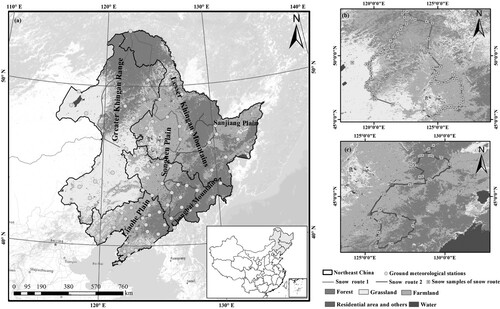
The location of Northeast China (115°30′ E–135°02′ E and 38°43′ N–53°36′N) is shown in Figure 1. Northeast China is the main snow cover region in China (Qi et al. 2020), the climate is controlled by the high-latitude East Asian monsoon, which includes warm temperate and cold temperate zones latitudinally, as well as semi-arid, semi-humid and humid zones from west to east. Winter is long and cold, with an annual average temperature range of 3–7°C. Besides, rainfall is generally concentrated from June to August (400–800 mm/year) (Li et al. 2022a). The terrain of Northeast China is complex and diverse, surrounded by mountains on three sides and high in elevation, with the Changbai Mountains in the east and the Lesser Khingan Mountains and Great Khingan Mountains in the north and west, respectively. The Sanjiang Plain, Songnen Plain and Liaohe Plain with flat terrain have fertile black soil and are important commodity grain bases in China. Furthermore, various types of land cover, such as farmland, grassland, and forests, are found in Northeast China. According to statistics, the forest cover in Northeast China exceeds 40% of its total area (Figure 1), which poses a serious challenge to SD inversion (Gu, Ren, and Li 2016; Guangrui et al. 2021).

Figure 1. Study area (a) Base map showing the land cover types, the spatial distribution of ground meteorological stations, and the field snow routes. (b) and (c) represent the distribution of SD observations along two snow routes.

2.2. Ground observation data

1. Meteorological station observations (Dataset 1)

The National Meteorological Information Centre, China Meteorology Administration (CMA, http://data.cma.cn/en) operates 91 ground meteorological stations in Northeast China. The spatial distribution of the stations is shown in Figure 1(a). The variables of the stations, including the name, geolocation (latitude and longitude), daily near-surface temperature (°C), daily SD (cm), and observation date, were collected. The SDs observed at daily near-surface temperatures below 0°C (273 K) were selected during the period 1987–2018. Accordingly, a total of 97,200 independent SD observations were collected during the study period during 2010–2018 and used to train the developed SD model. Moreover, a total of 201,696 independent SD observations made during the period 1987–2009 were used as ‘true’ data to estimate the accuracy of the developed model.

(2)	Snow route observation data (Dataset 2)

Dataset 2 relates to the SD samples used in the field snow survey experiment. Two snow survey routes (Figure 1(a)) were conducted between December 2017 and March 2018 in Northeast China under the Chinese snow survey project. A total of 102 snow samples were obtained from snow route 1 (Figure 1(b)), which were mainly distributed in farmland, grassland, and forest areas. Snow route 2 (Figure 1(c)), which included 60 snow samples, was located in the Lesser Khingan Mountains and Changbai Mountains. Dataset 2 was also used as the ‘ground-truth’ data for verification of the performance of the proposed model.

2.3. Enhanced resolution PMW data

The Calibrated Enhanced Resolution Brightness Temperature (CETB) data are available at https://nsidc.org/data/NSIDC-0630/versions/1 from 2018. They have been provided by the NASA Making Earth System Data Records for Use in Research Environments program (Brodzik, Long, and Hardman 2018). The original coarse-resolution TB data were gridded to obtain fine-resolution TB data using the scatterometer image reconstruction algorithm. The 19 and 22 GHz channels were reconstructed at a 6.25 km × 6.25 km spatial resolution, while the 37, 89, and 91 GHz channels were reconstructed at a 3.125 km × 3.125 km spatial resolution. The continuous CETB data from SSM/S and SSMIS radiometers could be downloaded from 1987. The CETB data at 19 and 37 GHz during the period from 1987 to 2018 were used in the study.

2.4. Other auxiliary data

It is important to understand spatiotemporal variations of snow cover characteristics (including snow density and snow grain size) in SD retrieving (Xu et al. 2022; Yang et al. 2021). In this study, the ERA5-land data with 10 km spatial resolution were employed to obtain the dynamic snow density. The air and soil temperatures obtained from ERA5-land data were used to indirectly characterize spatiotemporal variations of the snow grain size (see Section 3). The hourly ERA5-land data can be obtained at https://cds.climate.copernicus.eu. In addition, the land cover data with 500 m spatial resolution were required at https://search.earthdata.nasa.gov. The digital elevation model (DEM) data with 90 m spatial resolution were used in this paper, which could be obtained at http://srtm.csi.cgiar.org.

3. Method

3.1. Main variables’ preparation

The variables used in the study included ground in situ SD, CETB, snow cover characteristics, and environmental factors. We have listed these variables and their sources and contributions in Table 1.

Table 1. Summary of the datasets used in the study.

Named	Data source	Variables	Contributions
Meteorological station observations (Dataset 1)	The National Meteorological Information Centre, China Meteorology Administration	In-situ SD	Response variable; Model training (2010–2018)
			Model validation (1987–2009)
Snow route observation data (Dataset 2)	National Cryosphere Desert Data Center	In-situ SD	Model validation (2017–2018)
The enhanced resolution PMW data	National Snow and Ice Data Center	TB19H, TB37H	Prediction variables; Radiation information of snowpack in high resolution (1987–2018)
ERA5 – land data	The European Centre for Medium-range Weather Forecasts	Snow density, air temperature, soil temperature (0–7 cm)	Prediction variables; The information on snowpack metamorphism (1987–2018)
Land cover-type data	MODIS land cover data	Forest fraction (FF)	Prediction variables; The information on forest fraction (2001–2016)
Digital Elevation Model (DEM) data	The SRTM digital elevation data	Elevation, Slope, Aspect, Roughness	Prediction variables; The information on topographical features (2000)

Compared with the original PMW TB data at a 25 km resolution, the CETB data provide snowpack scattering information at a high spatial resolution (6.25 km × 6.25 km). Xiao et al. (Xiao et al. 2021) proved that the CETB data could provide a reliable data source for snow cover fraction assessment at a fine scale. We attempted to use these data to retrieve SD, improve the uncertainty caused by the coarse resolution, and restructure a fine-resolution SD dataset. Considering the influence of wet snow and the sensitivity of snow cover, only descending CETB data with horizontal (H) polarization (F08, F11, F13, and F17) were used in the study. Furthermore, to correspond to the spatial resolution at 19 GHz, the CETB at 37 GHz was aggregated to 6.25 km by averaging the surrounding four pixels.

The accuracy of SD assessment using PMW remote sensing is strongly related to snow characteristics, especially to snow grain size and density (Dai et al. 2022; Gao et al. 2022). However, temporally continuous and spatially distributed snow characteristics are usually unavailable at large spatial scales. According to ERA5-land data, daily snow density data can be employed as an input for the developed SD model. Besides, the temperature gradient (TG), expressed using Equation (1), can be used to indirectly characterize the spatiotemporal variations of the snow grain size. Previous studies have also shown that the TG is helpful a priori information for understanding the spatiotemporal distribution of snow grain size on continental scales (Xu et al. 2022). (1) $T{G}_d=Tsoi{l}_d-Tai{r}_d$(1) where $T{G}_d$, $Tsoi{l}_d$, and $Tai{r}_d$ represent the daily temperature gradient in snow cover, soil temperature in the upper layer, and air temperature, respectively, they could be extracted from hourly ERA5-land data. The snow density and TG were resampled to the 6.25 km spatial resolution using the nearest-neighbor interpolation method.

Vegetation-covered regions, especially in mountainous regions with complex terrain, are the main cause of errors found in SD retrieval (Che et al. 2016; Li and Kelly 2017). To overcome vegetation-related uncertainties, in our study, we calculated the forest fraction (FF) within each pixel of the CETB according to land cover type data. The FF maps from 2001 to 2016 were averaged into a single map to denote the average FF. In addition, the original DEM data were mosaicked and resampled to 6.25 km using nearest-neighbour interpolation. Subsequently, topographic factors, including elevation, slope, aspect, and roughness, were extracted using ArcGIS 10.4 to reduce the uncertainties of the complex terrain.

3.2. Random forest regression model

In our previous studies, we discussed the performance of different machine learning models, including support vector regression, XGboost, and RF regression, used in SD retrieval, and the results indicated that the RF regression model considerably outperformed the other machine learning regression models (Wei et al. 2022a; Wei et al. 2022b). The RF is an ensemble model based on decision trees. It can untangle the complex nonlinear relationship between the response variable and the prediction variables and was developed by Breiman (Breiman 2001). Before employing the RF regression model, the number of decision trees in the RF had to be typically defined. As stated by Yang et al. (Yang et al. 2020a), the number of decision trees was set to 1000 in this study. The other system parameters in the model were set to their default values. The RF regression model was obtained using the R package.

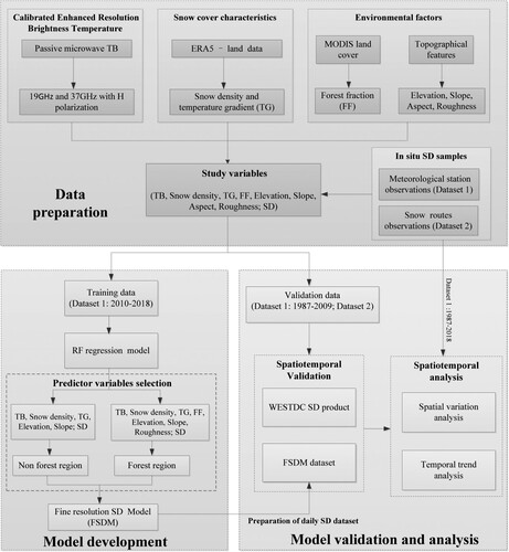
3.3. Development of the fine-resolution SD model

Because SD inversion is complex and affected by many factors, such as coarse spatial resolution, snow metamorphism, and environmental factors, we directly used the RF regression model to establish the nonlinear relationship between SD and relevant variables, including CETB, snow density, TG, FF, and topographical features (elevation, slope, aspect, and roughness). Previous studies have shown that the single SD retrieval model did not perform satisfactorily in Northeast China, especially in forest regions (Gu, Ren, and Li 2016; Wei et al. 2021b; Yang et al. 2020b). In this study, the developed SD retrieval model (called fine-resolution SD model, FSDM), was designed to be calibrated individually in forest regions to account for the spatiotemporal heterogeneity of the prediction variables. As shown in Equation (2) that the FSDM is divided into two parts based on the RF regression model: the non-forest region (FF ≤ 0.10) and the forest region (FF > 0.10). Dataset 1 of the period 2010–2018 was regarded as the response variable in the RF model for the training model, and the abovementioned variables were considered the input variables. The selection of the input variables will be explained in section 5. The main structure of the study is illustrated in Figure 2. (2) $FSDM=\{\begin{array}{c}RF(T{B}_{19H},T{B}_{19H},Snowdensity,TG,Elevation,Slope)FF\le 0.01\\ RF(T{B}_{19H},T{B}_{19H},Snowdensity,TG,FF,Elevation,Slope,Roughness)FF>0.01\end{array}$(2)

Figure 2. Schematic of the fine resolution SD retrieval model.

3.4. Evaluation indicators

The daily observed SD at 91 ground meteorological stations (Figure 1(a)) was used to evaluate the performances of the FSDM during the period 1987–2009. Additionally, Dataset 2, including 162 observations from the field snow survey experiment during 2017–2018, was also used as the truth SD observations to verify the stability of the FSDM in space. The RMSE, bias, and R were selected as the evaluation indicators to illustrate the inversion accuracy of the FSDM. The evaluation indicators were calculated using the following equations: (3) $RMSE=\sqrt{\sum _{\mathrm{i}=1}^N{(S{D}_0-S{D}_X)}^2/N}$(3) (4) $B\mathrm{i}\mathrm{a}\mathrm{s}=\sum _{\mathrm{i}=1}^N(S{D}_0-S{D}_X)/N$(4) (5) $R={\displaystyle \frac{\sum _{i=1}^N(S{D}_0-\overline{S{D}_0})(S{D}_X-\overline{S{D}_X})}{\sqrt{\sum _{i=1}^N{(S{D}_0-\overline{S{D}_0})}^2\sum _{i=1}^N{(S{D}_X-\overline{S{D}_X})}^2}}}$(5) where $S{D}_0$ and $S{D}_x$ represent the observed SD and retrieved SD, respectively, $\mathrm{N}$ is the number of SD samples. To show the spatiotemporal patterns of SD variation in Northeast China between 1987 and 2018, Sen’s slope estimator and the Mann-Kendall test (Gocic and Trajkovic 2013) were employed to analyze the SD variation trend.

4. Results

4.1. Validation and comparison of the FSDM dataset

A long-term, fine-resolution (with a spatial resolution of 6.25 km × 6.25 km), daily SD dataset was produced based on FSDM and evaluated using ground-truth SD observations from meteorological stations during the period 1987–2009. To avoid the influence of the wet snow cover, the FSDM dataset of the main snowy winter season (October–April) was selected. The SDs observed at daily near-surface temperatures below 0°C (273 K) were used for validation. The SDs retrieved at air temperatures below 0°C (273 K) were used for dataset preparation. Furthermore, the FSDM dataset was also compared with the traditional empirical algorithm developed by Che et al. (Che et al. 2008) in China. The existing SD dataset at a 25 km spatial resolution could be acquired from the Environmental and Ecological Science Data Center for West China (http://westdc.westgis.ac.cn), hereinafter referred to as WESTDC. Because the WESTDC SD product has been widely used for SD evaluation and analysis (Che et al. 2016; Dai and Che 2014; Ma et al. 2020; Yang et al. 2020a), it was better to demonstrate the performance of the FSDM dataset by comparing with WESTDC product.

Figure 3 shows density scatterplots of the retrieved SD and the observed SD during the snow season from 1987 to 2009. As seen, the FSDM dataset had better consistency with observed SD (Figure 3(a)), and the accuracy was superior to the WESTDC product, with RMSE, bias, and R of 7.10 cm, −0.13 cm, and 0.60, respectively. The RMSE, bias, and R of the WESTDC SD product were 8.08 cm, −0.62 cm, and 0.43, respectively (Figure 3(b)). Furthermore, the error bar in Figure 3 indicates that two SD products underestimated observed SD under deep snowpacks. To explore the performance of two SD products under deep snowpack conditions, we selected 25 cm as the threshold to assess the performances in shallow (≤25 cm) and deep (>25 cm) snowpacks. Table 2 displays the comparison between FSDM data and the WESTDC product in deep and shallow snow covers. In a shallow snowpack, the overall accuracy of the FSDM dataset was higher than that of the WESTDC product, the RMSE, bias, and R were 6.36, 0.51 cm, and 0.62, respectively. In the deep snowpack, the FSDM dataset and WESTDC product demonstrated significant underestimation with a bias of −12.42 cm and −13.60 cm, respectively. However, when we checked the SD observation samples, we found that shallow snowpack conditions account for approximately 95% of total SD samples, and deep snow conditions account for approximately only 5% of all samples in Northeast China.

Figure 3. Density scatterplots of the retrieved SD and the observed SD during the period 1987–2009. (a) FSDM dataset and (b) WESTDC product.

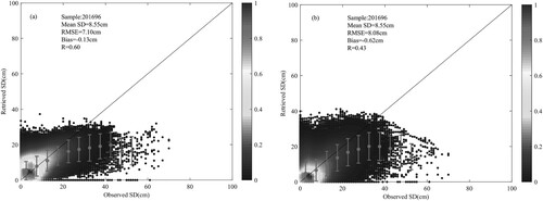
Table 2. Comparison between the FSDM dataset and WESTDC SD product for shallow (≤25 cm) and deep (>25 cm) snow covers.

Name	FSDM		WESTDC
SD (cm)	≤25	>25	≤25	>25
RMSE (cm)	6.36	15.74	7.33	16.11
Bias (cm)	0.51	−12.42	−0.52	−13.60
R	0.62	0.14	0.46	0.12
Samples	SD ≤ 25 cm: 192461 (95%)		SD > 25 cm: 9235 (5%)

Figure 4 shows the spatial distribution of RMSEs of the FSDM dataset and WESTDC product from the validations against the observed SD data at 91 meteorological stations in Northeast China. The results suggested that the RMSEs of the FSDM dataset were lower than those of the WESTDC SD product in most stations, the FSDM dataset effectively improved the accuracy of SD inversion in mountainous areas (Figure 4(a)). However, we found that the FSDM dataset and WESTDC product still had higher RMSE in forest areas, and the RMSE of WESTDC products was higher than that of the FSDM dataset. We compared the SD retrieval accuracy of the FSDM dataset and WESTDC product in forest and non-forest areas, as shown in Table 3. The results have shown that the overall accuracy of the FSDM dataset and WESTDC product was lower in forest regions than in non-forest regions. However, the overall accuracy of the FSDM dataset was higher than that of the WESTDC product, with the RMSE, bias, and R of 6.56 cm, −0.41 cm and 0.69 in non-forest regions, with the RMSE, bias, and R of 7.78, 0.24 cm, and 0.47 in forest regions.

Figure 4. Spatial patterns of the RMSE of the (a) FSDM dataset and (b) WESTDC product from the validations against the observed SD data from 91 meteorological stations in Northeast China.

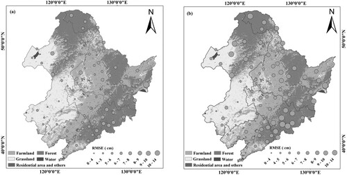
Table 3. RMSE, bias, and R of the FSDM dataset and WESTDC product in non-forest and forest regions.

Name	FSDM		WESTDC
	Non-forest	Forest	Non-forest	Forest
RMSE (cm)	6.56	7.78	7.36	8.96
Bias (cm)	−0.41	0.24	−0.42	−0.88
R	0.69	0.47	0.53	0.36
Mean SD (cm)	Non-Forest: 7.54 cm		Forest: 10.90 cm

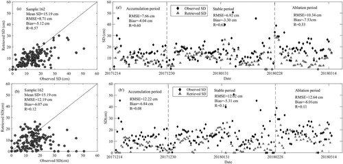
To investigate the stability of the FSDM dataset, we analyzed the agreement between the retrieved SD and observed SD based on snow survey routes. Figure 5 shows the results of the validation of the two SD products against Dataset 2, the results from Figure 5(a) and (b) show that the FSDM dataset had better stability compared with the WESTDC product because of considering the spatiotemporal variation of snowpack characteristics, with RMSE, bias, and R were 8.71 cm, −5.12 cm, and 0.57, respectively. The WESTDC product had large uncertainties, with RMSE, bias, and R of 12.19 cm, −6.07 cm, and 0.12, respectively. Furthermore, we analyzed the performance of the FSDM dataset and WESTDC product in time series. Figure 5(a’) and (b’) represent the scatter diagrams of the FSDM dataset and WESTDC product from the validations against snow routes in time series, the results indicated that the two products had better consistency with the observed SD during snow stable period than accumulation and ablation periods. This is mainly because the snowpack was dry in the stable period, the snow characteristics were relatively stable, and the surface radiation signal was less disturbed by the snowpack characteristics.

Figure 5. Scatter plots of retrieved SD and observed SD based on Dataset 2. (a) and (b) represent the FSDM and WESTDC, respectively; (a’) and (b’) represent the comparison result along the observation time.

4.2. Spatial patterns of the SD from the FSDM datasets

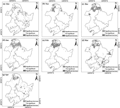
The abovementioned results suggested that the FSDM dataset had satisfactory accuracy and stability. In this section, we analyze the spatial patterns of the FSDM dataset during the period 1987–2018. Figure 6 presents the spatial distributions of the monthly SDs in Northeast China. The results show that the snow cover is mainly distributed in the Greater Khingan Range, Lesser Khingan Mountains, and Changbai Mountain regions, and the SD exhibited high-low distribution patterns with latitude. The snow cover appeared in the Greater Khingan Range in October and disappeared in April in most regions. The maximum SD value occurred in the Greater Khingan Range in February. In the whole snow season, the SD in Liaohe Plain was the smallest, because the air temperature was high in Liaohe Plain, resulting in late snowing and early melting. Figure 7 shows the spatial distribution of the multiyear (1987–2018) mean monthly SD change trends from October to April. From a visual perspective, the spatial distribution of the SD change trends had obvious heterogeneity in Northeast China, and the changing trend of SD in different months also had significant differences. For example, in October, January, February, and April, the changing trends of SD decreased in most parts of the Changbai Mountains, whereas the changing trends of SD increased in November, December, and March. Except for October, the changing trends of the mean monthly SD decreased in the north of Northeast China. However, Figure 8 shows that the change trends of the monthly SD were not significant in most parts of Northeast China.

Figure 6. Spatial variations of the multiyear (1987–2018) mean monthly SD from October to April in Northeast China based on the FSDM dataset.

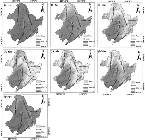
Figure 7. Spatial distribution of the multiyear (1987–2018) mean monthly SD change trends from October to April in Northeast China based on the FSDM dataset.

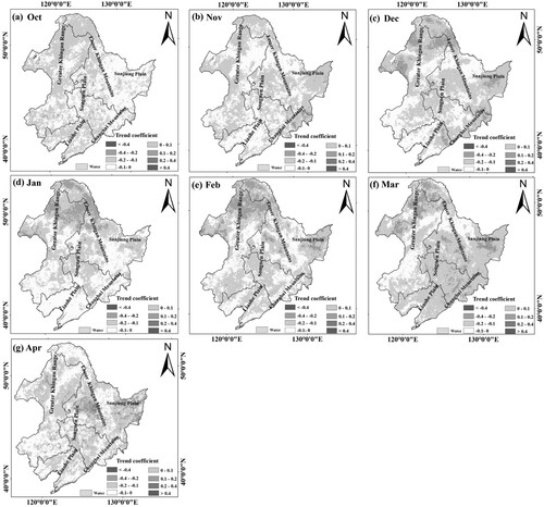
Figure 8. Spatial distribution of the multiyear (1987–2018) mean monthly SD significance test from October to April in Northeast China based on the FSDM dataset. The variation trend is regarded as statistically significant when p < 0.05.

4.3. Temporal variation of SD from the FSDM dataset

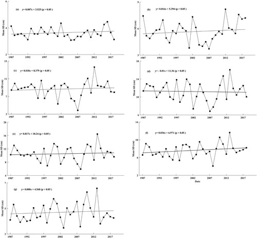
Figure 9 shows the interannual variations and linear trends of the monthly SDs during 1987–2018. In the case of interannual variations, the fluctuation range of annual average SD tends to be stable, for example, the interannual mean SD fluctuated between 3 and 5 cm in October (Figure 9(a)), and fluctuated between 3 and 7 cm in April (Figure 9(g)). But the fluctuation range of the annual average SD was significant in January (6–18 cm) and February (4–17 cm). In the case of change trends, except for February, the interannual mean SD in other months showed an increase trend, and the increase trend was highest in March with a rate of 0.036 cm/year (p > 0.05). The annual mean SD increased slightly with a rate of 0.007 in October. In February, the annual mean SD decreased slightly with a rate of −0.01 cm/year (p > 0.05). However, the variation trends of the mean monthly SD were not significant during 1987–2018.

Figure 9. The interannual variations and the linear trends of the mean monthly SD from October to April during 1987–2018.

5. Discussion

5.1. The selection of the input variables in FSDM

In the FSDM, nine types of input variables, namely, TB at 37H and 19H, FF, TG, snow density, elevation, slope, aspect, and roughness are selected as the input variables for SD retrieval. Each type of input variable can provide a priori knowledge from specific perspectives, as shown in Table 2. Figure 10(a) and (b) demonstrate the importance of the input variables to FSDM performance in non-forest and forest regions, respectively. The results indicate that all input variables contribute to the improvement of the SD accuracy of the FSDM at varying degrees. However, to determine the optimal input features and make the training procedure simple without sacrificing prediction accuracy, the redundant predictor variables have to be filtered out.

Figure 10. Importance of the input variables for FSDM performance in (a) non-forest regions and (b) forest regions.

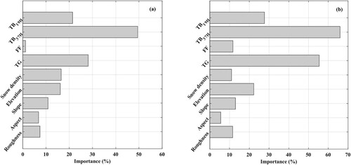
Accordingly, we applied the 10-fold CV strategies to the training dataset to demonstrate FSDM performance. First, only TB at 19 and 37 H without auxiliary data were used as the input variables to test the effectiveness of the FSDM. Thereafter, we added different types of variables to the FSDM and tested its performance. If during this process, the RMSE decreased and R increased, then the selected input variables are considered to be effective for SD assessment. Tables 4 and 5 show the performance of the FSDM based on different feature combinations in non-forest and forest regions, respectively. The RMSEs of the M1 are 6.30 and 8.21 cm in non-forest and forest regions, respectively, and R was less than 0.60. When the FF factor was included, the FSDM demonstrated better performance in forest regions than when the FF factor was excluded, as shown in Table 5 for M2. However, the FF factor does not effectively improve the FSDM performance in non-forest regions and may even play a negative role (M2 in Table 4). When we included the variables TG, FF, snow density, elevation, and slope in the FSDM individually, as shown for M6 in Tables 4 and 5, the SD estimation accuracy based on FSDM showed a significant improvement, with the RMSE decreasing by ∼ 2 cm in the non-forest and forest regions, respectively. The inclusion of the two variables, aspect and roughness, does not improve FSDM performance in non-forest regions (M7 and M8 in Table 4), but the inclusion of roughness contributed to improving the SD estimates in forest regions (M8 in Table 5). Accordingly, as the input variables of FSDM, we selected TB, TG, snow density, elevation, and slope for the non-forest regions and TB, FF, TG, snow density, elevation, slope, and roughness for the forest regions, as shown in Equation (2).

Table 4. Detailed error statistics of the FSDM in non-forest regions based on different feature combinations.

Models	Input variables	Non-forest regions (10-fold CV in training dataset)
		RMSE (cm)	Bias (cm)	R
M 1	TB at 19H and 37H	6.30	−0.62	0.58
M 2	TB + FF	6.32	−0.64	0.58
M 3	TB + TG	5.80	−0.50	0.67
M 4	TB + TG + snow density	5.63	−0.45	0.71
M 5	TB + TG + snow density + Elevation	4.55	−0.60	0.82
M 6	TB + TG + snow density + Elevation + Slope	4.38	−0.38	0.84
M 7	TB + TG + snow density + Elevation + Slope + Aspect	4.38	−0.34	0.84
M 8	TB + TG + snow density + Elevation + Slope + Roughness	4.39	−0.31	0.84

Table 5. Detailed error statistics of the FSDM in forest regions based on different feature combinations.

Models	Input Variables	Forest regions (10-fold CV in training dataset)
		RMSE (cm)	Bias (cm)	R
M 1	TB at 19H and 37H	8.21	−2.02	0.54
M 2	TB + FF	7.62	−2.10	0.63
M 3	TB + FF + TG	7.00	−1.95	0.67
M 4	TB + FF + TG + snow density	6.85	−1.49	0.70
M 5	TB + FF + TG + snow density + Elevation	6.22	−1.31	0.74
M 6	TB + FF + TG + snow density + Elevation + Slope	6.17	−1.22	0.74
M 7	TB + FF + TG + snow density + Elevation + Slope + Aspect	6.19	−1.25	0.74
M 8	TB + FF + TG + snow density + Elevation + Slope + Roughness	6.12	−1.01	0.75

5.2. Detailed advantages of the FSDM

In the studies mentioned, the accuracy and stability of the FSDM dataset were verified and the spatiotemporal changes in Northeast China were analyzed using the FSDM dataset. In this section, we compared the temporal and spatial changes of SD using FSDM and WESTDC datasets in Northeast China and discussed the differences between FSDM and WESTDC datasets for further illustrating the potential capability of FSDM in revealing spatiotemporal variations of snow cover at a fine scale. Figure 11(a) and (b) show the variation trends of the FSDM dataset and WESTDC product during the period 1987–2018. Generally, the two SD datasets exhibited similar variation trends. The annual SD increased slightly at a rate of 0.029 cm/year (p > 0.05) in the FSDM dataset and at a rate of 0.027 cm/year (p > 0.05) in the WESTDC product. The maximum SD values (exceeding 10 cm) were recorded in 2017, while the minimum SD values (below 5 cm) were recorded in 2007 for two datasets. We also show the spatial pattern of the annual SD variation. Figure 12(a) and (b) represent the variations of the SD spatial pattern of the FSDM dataset and WESTDC product during 1987-2018, respectively. The results show that the variations of the annual SD were not significant in most parts of Northeast China. However, compared with the WESTDC product, the FSDM dataset exhibited a fine spatial pattern.

Figure 11. Mean annual SD variation of the (a) FSDM dataset and (b) WESTDC product during 1987–2018 in Northeast China.

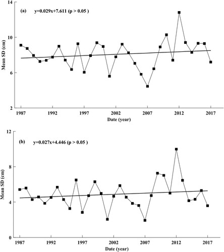
Figure 12. Variation trends of the SD from 1987 to 2018. (a) and (b) represent the variations of the SD spatial pattern of the FSDM dataset and WESTDC product, respectively. (a) and (b) represent the spatial patterns of the trend changes from the FSDM dataset and the WESTDC product, respectively. (c) shows the similarity and differences between the FSDM dataset and the WESTDC product, and the pie chart at the bottom right represents the proportion of the similarity/difference areas in the total area.

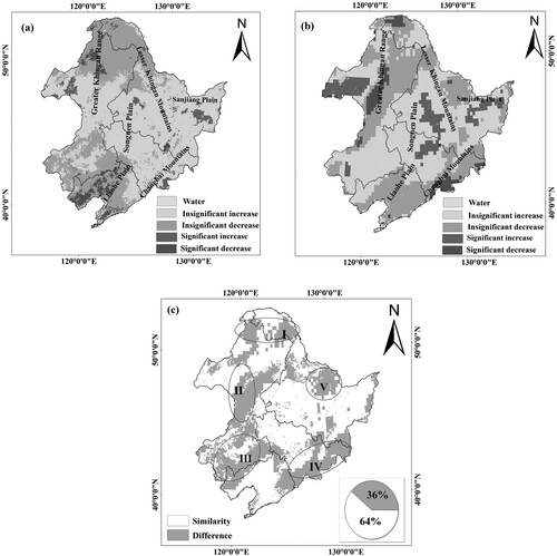
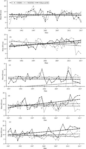
Meanwhile, Figure 12(c) shows the similarity and difference in variation trends between the FSDM dataset and the WESTDC product. Generally, the variation trends of SD were the same in most areas (more than 60% of the total region) between the FSDM dataset and the WESTDC product. However, we could see from Figure 12(c) that there were significant differences in SD variation trends between FSDM and WESTDC products. For example, in the northern part of the Lesser Khingan Mountains, the FSDM product recorded a decreasing trend in the SD (Figure 12 (a)), whereas the WESTDC product recorded an increasing trend in the SD (Figure 12 (b)). In the southern Changbai Mountains, an increasing trend of the SD was shown by the FSDM product, whereas a decreasing trend of the SD was shown by the WESTDC product. Based on the comparison of trends in Figure 12 and ground meteorological station observations in Figure 1, we selected 5 specific regions (the black circle in Figure 12 (c)) to check the variation trend of SD. Figure 13 shows the variation trends of SD based on the ground meteorological station observations (black line), FSDM dataset (orange line), and WESTDC product (blue line). The results show that the changing trends of the SD had good consistency between FSDM datasets and ground observation stations. However, the variation trends of the SD were different between the WESTDC product and station observations.

Figure 13. Variation trend analysis of the SD in five regions based on station observations, FSDM dataset, and WESTDC product.

5.3. Potential errors in the FSDM dataset

The FSDM dataset has satisfactory accuracy and stability, and it can accurately reveal the spatiotemporal variations of SD at fine resolution, which will contribute to hydrological and climatological studies conducted in continuous watersheds. However, the FSDM dataset has several limitations. Figure 3 and Table 2 show that the FSDM does not effectively solve the problem of underestimation in deep snowpack conditions (SD > 25 cm), the value of the bias was −12.42 cm for deep snowpack, which may be due to the TB reaching a saturation threshold and does not tend to monotonically decrease with an increase in the SD when SD in deep condition. However, because deep snow samples constitute only 5% of all the samples (Table 2), the FSDM still has extensive applications in Northeast China.

Figure 6 shows that the snow cover is mainly distributed in mountainous areas with a dense forest cover and complex terrain environments, including the Greater Khingan Range, the Lesser Khingan Mountains, and the Changbai Mountain regions. Although the FF and topographical features were included to reduce the impact of the forest attenuation and complex terrains and they achieved lower RMSEs in FSDM. Figure 4 and Table 3 indicate that the FSDM did not perform as well in complex mountainous areas as in the other regions (such as farmland), which may be due to the following reasons. First, forest cover attenuation with a high degree of complexity is related to not only the FF but also forest types, forest biomass, and tree canopy size (Gu, Ren, and Li 2016; Guangrui et al. 2021). Secondly, because the physical explanation that how the complex terrain in mountainous regions alters the radiative transfer of microwave emission is still unclear for machine learning models, it is still challenging to model the spatial variation and temporal evolution of SD in mountainous regions (Li, Durand, and Margulis 2012). Thirdly, an uncertain factor in SD inversion is the presence of liquid water. Yang et al. (Yang et al. 2020a) showed that large errors in SD assessment always occur in the late snow season. When the snow begins to melt, the snowpack tends to undergo frequent freeze–thaw cycles which leads to the evolution of the snow characteristics. Therefore, it is impossible to retrieve SD based on PMW under wet snow conditions (Che et al. 2014).

6. Conclusion

An accurate, reliable, high-resolution, and long-term SD dataset is essential for hydrological process monitoring and climate modeling applications. To overcome the uncertainties derived from coarse spatial resolution, snowpack metamorphism, complex terrain, and vegetation cover in SD inversion, this study developed an FSDM by combining the CETB data and other auxiliary information (e.g. snow cover characteristics and environmental factors), and produced a long-term, fine-resolution daily SD dataset for the period 1987–2018. Instead of complex physical models, the RF regression model was used to untangle the nonlinear complex relationship between SD and other auxiliary information, and a zoning modeling strategy was employed in the FSDM to reduce the bias caused by snow heterogeneity in forest regions. The validation against 91 ground meteorological stations and 162 SD observations in snow routes shows that the FSDM dataset achieves satisfactory accuracy and stability and that it significantly improves both spatial resolution and retrieval accuracy compared with traditional empirical algorithms.

Using the FSDM dataset, we found that the snow cover was mainly distributed in the Greater Khingan Range, Lesser Khingan Mountains, and Changbai Mountain regions and the SD showed a high-low distribution pattern with latitude. The snow cover appeared in the Greater Khingan Range in October and disappeared in April in most regions. The maximum SD value occurred in the Greater Khingan Range in February. In the whole snow season, the SD in Liaohe Plain was the smallest. The spatial distribution of the SD change trends had obvious heterogeneity, and the changing trends in different months also had significant differences. In October, January, February, and April, the SD decreased in most parts of the Changbai Mountains, whereas it increased in November, December, and March. Except for October, the changing trends of the mean monthly SD decreased in the north of Northeast China. Furthermore, the annual mean SD showed a slightly increasing trend (p > 0.05) at a rate of 0.029 cm/year during 1987–2018. However, the variation trends of SD are not significant in most parts of Northeast China.

Like the existing SD products, the FSDM dataset also has limitations, i.e. underestimation of deep snowpack. The FSDM did not perform as well in complex mountainous areas as in the other regions (such as non-forest regions) because of the high complexity of microwave radiation in forest regions. Future studies may incorporate the physical model to separate the contributions of complex terrains to TB. In this way, we can not only achieve accurate SD assessment but also gather the physical details of the radiative transfer of microwave emissions in mountainous regions. In addition, the presence of liquid water in the snowpack can cause more errors in SD assessment. Therefore, an accurate snow cover detection method should be developed to filter out the wet snow cover in future studies.

Disclosure statement

No potential conflict of interest was reported by the author(s).

Additional information

Funding

This work was supported by Strategic Priority Research Program of the Chinese Academy of Sciences [grant number XDA28110502]; National Natural Science Foundation of China [grant number 41871248]; Changchun Science and Technology Development Plan Project [grant number 21ZY12]; Innovation and Entrepreneurship Talent Project of Jilin Province [grant number 2023QN15].

References

- Barnett, T. P., J. C. Adam, and D. P. Lettenmaier. 2005. “Potential Impacts of a Warming Climate on Water Availability in Snow-Dominated Regions.” Nature 438 (7066): 303–309. doi:10.1038/nature04141.
- Bhatti, Asif M., Toshio Koike, and Maheswor Shrestha. 2016. “Climate Change Impact Assessment on Mountain Snow Hydrology by Water and Energy Budget-Based Distributed Hydrological Model.” Journal of Hydrology 543: 523–541. doi:10.1016/j.jhydrol.2016.10.025.
- Breiman. 2001. “Random Forests.” Machine Learning 45 (1): 5–32. doi:10.1023/A:1010933404324.
- Brodzik, Mary J., David G. Long, and Molly A. Hardman. 2018. “Best Practices in Crafting the Calibrated, Enhanced-Resolution Passive-Microwave EASE-Grid 2.0 Brightness Temperature Earth System Data Record.” Remote Sensing 10 (11): 1793. doi:10.3390/rs10111793
- Chang, A. T. C., J. L. Foster, and D. K. Hall. 1987. “Nimbus-7 SMMR Derived Global Snow Cover Parameters.” Annals of Glaciology 9: 39–44. doi:10.1017/S0260305500200736
- Che, Tao, Liyun Dai, Xingming Zheng, Xiaofeng Li, and Kai Zhao. 2016. “Estimation of Snow Depth from Passive Microwave Brightness Temperature Data in Forest Regions of Northeast China.” Remote Sensing of Environment 183: 334–349. doi:10.1016/j.rse.2016.06.005.
- Che, Tao, Xin Li, Rui Jin, and Chunlin Huang. 2014. “Assimilating Passive Microwave Remote Sensing Data Into a Land Surface Model to Improve the Estimation of Snow Depth.” Remote Sensing of Environment 143: 54–63. doi:10.1016/j.rse.2013.12.009.
- Che, Tao, Li Xin, Jin Rui, Richard Armstrong, and Tingjun Zhang. 2008. “Snow Depth Derived from Passive Microwave Remote-Sensing Data in China.” Annals of Glaciology 49 (1): 145–154. doi:10.3189/172756408787814690.
- Dai, L., and T. Che. 2014. “Spatiotemporal Variability in Snow Cover from 1987 to 2011 in Northern China.” Journal of Applied Remote Sensing 8 (1): 084693. doi:10.1117/1.JRS.8.084693.
- Dai, Liyun, Tao Che, Yongjian Ding, and Xiaohua Hao. 2017. “Evaluation of Snow Cover and Snow Depth on the Qinghai-Tibetan Plateau Derived from Passive Microwave Remote Sensing.” The Cryosphere 11 (4): 1933–1948. doi:10.5194/tc-11-1933-2017.
- Dai, L., T. Che, L. Xiao, M. Akynbekkyzy, K. Zhao, and L. Leppänen. 2022. “Improving the Snow Volume Scattering Algorithm in a Microwave Forward Model by Using Ground-Based Remote Sensing Snow Observations.” IEEE Transactions on Geoscience and Remote Sensing 60: 1–17. doi:10.1109/TGRS.2021.3064309.
- Dai, Liyun, Tao Che, Hongjie Xie, and Xuejiao Wu. 2018. “Estimation of Snow Depth Over the Qinghai-Tibetan Plateau Based on AMSR-E and MODIS Data.” Remote Sensing 10 (12): 1989. doi:10.3390/rs10121989.
- Derksen, C., P. Toose, A. Rees, L. Wang, M. English, A. Walker, and M. Sturm. 2010. “Development of a Tundra-Specific Snow Water Equivalent Retrieval Algorithm for Satellite Passive Microwave Data.” Remote Sensing of Environment 114 (8): 1699–1709. doi:10.1016/j.rse.2010.02.019.
- Estilow, T. W., A. H. Young, and D. A. Robinson. 2015. “A Long-Term Northern Hemisphere Snow Cover Extent Data Record for Climate Studies and Monitoring.” Earth System Science Data 7 (1): 137–142. doi:10.5194/essd-7-137-2015.
- Foster, J. L., A. T. C. Chang, and D. K. Hall. 1997. “Comparison of Snow Mass Estimates from a Prototype Passive Microwave Snow Algorithm, a Revised Algorithm and a Snow Depth Climatology.” Remote Sensing of Environment 62 (2): 132–142. doi:10.1016/S0034-4257(97)00085-0.
- Gao, S., Z. Li, P. Zhang, Q. Chen, J. Zeng, C. Zhao, C. Liu, and Z. Zheng. 2022. “Global Sensitivity Analysis of the MEMLS Model for Retrieving Snow Water Equivalent.” IEEE Transactions on Geoscience and Remote Sensing 60: 1–15. doi:10.1109/TGRS.2021.3134695.
- Gocic, M., and S. Trajkovic. 2013. “Analysis of Changes in Meteorological Variables Using Mann-Kendall and Sen’s Slope Estimator Statistical Tests in Serbia.” Global & Planetary Change 100 (JAN.): 172–182. doi:10.1016/j.gloplacha.2012.10.014.
- Gu, Lingjia, Ruizhi Ren, and Xiaofeng Li. 2016. “Snow Depth Retrieval Based on a Multifrequency Dual-Polarized Passive Microwave Unmixing Method from Mixed Forest Observations.” IEEE Transactions on Geoscience and Remote Sensing 54 (12): 7279–7291. doi:10.1109/TGRS.2016.2599013.
- Guangrui, Wang, Li Xiaofeng, Chen Xiuxue, Jiang Tao, Zheng Xingming, Wei Yanlin, Wan Xiangkun, and Wang Jian. 2021. “An Investigation on Microwave Transmissivity at Frequencies of 18.7 and 36.5 GHz for Diverse Forest Types During Snow Season.” International Journal of Digital Earth 14 (10): 1354–1379. doi:10.1080/17538947.2021.1955985.
- Hao, Xiaohua, Guanghui Huang, Tao Che, Wenzheng Ji, Xingliang Sun, Qin Zhao, Hongyu Zhao, Jian Wang, Hongyi Li, and Qian Yang. 2021. “The NIEER AVHRR Snow Cover Extent Product Over China – A Long-Term Daily Snow Record for Regional Climate Research.” Earth System Science Data 13 (10): 4711–4726. doi:10.5194/essd-13-4711-2021.
- Hori, M., K. Sugiura, K. Kobayashi, T. Aoki, T. Tanikawa, K. Kuchiki, M. Niwano, and H. Enomoto. 2017. “A 38-Year (1978–2015) Northern Hemisphere Daily Snow Cover Extent Product Derived Using Consistent Objective Criteria from Satellite-Borne Optical Sensors.” Remote Sensing of Environment 191: 402–418. doi:10.1016/j.rse.2017.01.023.
- Hu, Y., T. Che, L. Dai, Y. Zhu, L. Xiao, J. Deng, and X. Li. 2022. “A Long-Term Daily Gridded Snow Depth Dataset for the Northern Hemisphere from 1980 to 2019 Based on Machine Learning.” Earth System Science Data Discuss 2022: 1–33. doi:10.5194/essd-2022-63.
- Huang, Xiaodong, Jie Deng, Xiaofang Ma, Yunlong Wang, Qisheng Feng, Xiaohua Hao, and Tiangang Liang. 2016. “Spatiotemporal Dynamics of Snow Cover Based on Multi-Source Remote Sensing Data in China.” The Cryosphere 10 (5): 2453–2463. doi:10.5194/tc-10-2453-2016.
- Iwata, Y., M. Hayashi, S. Suzuki, T. Hirota, and S. Hasegawa. 2010. “Effects of Snow Cover on Soil Freezing, Water Movement, and Snowmelt Infiltration: A Paired Plot Experiment.” Water Resources Research 46 (9). doi:10.1029/2009WR008070.
- Kelly, Richard. 2009. “The AMSR-E Snow Depth Algorithm: Description and Initial Results.” Journal of the Remote Sensing Society of Japan 29 (1): 307–317. doi:10.11440/rssj.29.307.
- Kelly, R. E., A. T. Chang, Leung Tsang, and J. L. Foster. 2003. “A Prototype AMSR-E Global Snow Area and Snow Depth Algorithm.” IEEE Transactions on Geoscience and Remote Sensing 41 (2): 230–242. doi:10.1109/TGRS.2003.809118.
- Li, Dongyue, Michael Durand, and Steven A. Margulis. 2012. “Potential for Hydrologic Characterization of Deep Mountain Snowpack via Passive Microwave Remote Sensing in the Kern River Basin, Sierra Nevada, USA.” Remote Sensing of Environment 125: 34–48. doi:10.1016/j.rse.2012.06.027.
- Li, Qinghuan, and Richard E. J. Kelly. 2017. “Correcting Satellite Passive Microwave Brightness Temperatures in Forested Landscapes Using Satellite Visible Reflectance Estimates of Forest Transmissivity.” IEEE Journal of Selected Topics in Applied Earth Observations and Remote Sensing 10 (9): 3874–3883. doi:10.1109/JSTARS.2017.2707545.
- Li, Lei, Xiaofeng Li, Xingming Zheng, Xiaojie Li, Tao Jiang, Hanyu Ju, and Xiangkun Wan. 2022a. “The Effects of Declining Soil Moisture Levels on Suitable Maize Cultivation Areas in Northeast China.” Journal of Hydrology 608: 127636. doi:10.1016/j.jhydrol.2022.127636.
- Li, Yanxin, Deping Liu, Tianxiao Li, Qiang Fu, Dong Liu, Renjie Hou, Fanxiang Meng, Mo Li, and Qinglin Li. 2022b. “Responses of Spring Soil Moisture of Different Land Use Types to Snow Cover in Northeast China Under Climate Change Background.” Journal of Hydrology 608: 127610. doi:10.1016/j.jhydrol.2022.127610.
- Li, Xiaofeng, Kai Zhao, Lili Wu, Xingming Zheng, and Tao Jiang. 2014. “Spatiotemporal Analysis of Snow Depth Inversion Based on the FengYun-3B MicroWave Radiation Imager: A Case Study in Heilongjiang Province, China.” Journal of Applied Remote Sensing 8 (1). doi:10.1117/1.JRS.8.084692.
- Luojus, Kari, Jouni Pulliainen, Matias Takala, Juha Lemmetyinen, Colleen Mortimer, Chris Derksen, Lawrence Mudryk, et al. 2021. “GlobSnow v3.0 Northern Hemisphere Snow Water Equivalent Dataset.” Scientific Data 8 (1): 163. doi:10.1038/s41597-021-00939-2.
- Ma, Ning, Kunlun Yu, Yinsheng Zhang, Jianqing Zhai, Yongqiang Zhang, and Hongbo Zhang. 2020. “Ground Observed Climatology and Trend in Snow Cover Phenology Across China with Consideration of Snow-Free Breaks.” Climate Dynamics 55 (9): 2867–2887. doi:10.1007/s00382-020-05422-z.
- Matiu, M., A. Crespi, G. Bertoldi, C. M. Carmagnola, C. Marty, S. Morin, W. Schöner, et al. 2021. “Observed Snow Depth Trends in the European Alps: 1971 to 2019.” The Cryosphere 15 (3): 1343–1382. doi:10.5194/tc-15-1343-2021.
- Pulliainen, Jouni, Kari Luojus, Chris Derksen, Lawrence Mudryk, Juha Lemmetyinen, Miia Salminen, Jaakko Ikonen, et al. 2020. “Patterns and Trends of Northern Hemisphere Snow Mass from 1980 to 2018.” Nature 581 (7808): 294–298. doi:10.1038/s41586-020-2258-0.
- Qi, Wei, Lian Feng, Junguo Liu, and Hong Yang. 2020. “Snow as an Important Natural Reservoir for Runoff and Soil Moisture in Northeast China.” Journal of Geophysical Research: Atmospheres 125 (22): e2020JD033086. doi:10.1029/2020JD033086.
- Qin, Yue, John T. Abatzoglou, Stefan Siebert, Laurie S. Huning, Amir AghaKouchak, Justin S. Mankin, Chaopeng Hong, Dan Tong, Steven J. Davis, and Nathaniel D. Mueller. 2020. “Agricultural Risks from Changing Snowmelt.” Nature Climate Change 10 (5): 459–465. doi:10.1038/s41558-020-0746-8
- Slater, A. G., A. P. Barrett, M. P. Clark, J. D. Lundquist, and M. S. Raleigh. 2013. “Uncertainty in Seasonal Snow Reconstruction: Relative Impacts of Model Forcing and Image Availability.” Advances in Water Resources 55: 165–177. doi:10.1016/j.advwatres.2012.07.006.
- Wang, Yunlong, Xiaodong Huang, Jianshun Wang, Minqiang Zhou, and Tiangang Liang. 2019. “AMSR2 Snow Depth Downscaling Algorithm Based on a Multifactor Approach Over the Tibetan Plateau, China.” Remote Sensing of Environment 231: 111268. doi:10.1016/j.rse.2019.111268.
- Wei, Yanlin, Xiaofeng Li, Lingjia Gu, Ming xing Zheng, Tao Jiang, Xiaojie Li, and Xiangkun Wan. 2021a. “A Dynamic Snow Depth Inversion Algorithm Derived from AMSR2 Passive Microwave Brightness Temperature Data and Snow Characteristics in Northeast China.” IEEE Journal of Selected Topics in Applied Earth Observations and Remote Sensing 14: 1–2. doi:10.1109/JSTARS.2021.3050573.
- Wei, Y., X. Li, L. Gu, X. Zheng, T. Jiang, and Z. Zheng. 2022a. “A Fine-Resolution Snow Depth Retrieval Algorithm from Enhanced-Resolution Passive Microwave Brightness Temperature Using Machine Learning in Northeast China.” IEEE Geoscience and Remote Sensing Letters 19: 1–5. doi:10.1109/LGRS.2022.3196135.
- Wei, Yanlin, Xiaofeng Li, Li Li, Lingjia Gu, Xingming Zheng, Tao Jiang, and Xiaojie Li. 2022b. “An Approach to Improve the Spatial Resolution and Accuracy of AMSR2 Passive Microwave Snow Depth Product Using Machine Learning in Northeast China.” Remote Sensing 14 (6): 1480. doi:10.3390/rs14061480.
- Wei, Pengtao, Tingbin Zhang, Xiaobing Zhou, Guihua Yi, Jingji Li, Na Wang, and Bo Wen. 2021b. “Reconstruction of Snow Depth Data at Moderate Spatial Resolution (1 km) from Remotely Sensed Snow Data and Multiple Optimized Environmental Factors: A Case Study Over the Qinghai-Tibetan Plateau.” Remote Sensing 13 (4): 1–21. doi:10.3390/rs13040657.
- Xiao, X., S. Liang, T. He, D. Wu, and J. Gong. 2021. “Estimating Fractional Snow Cover from Passive Microwave Brightness Temperature Data Using MODIS Snow Cover Product Over North America.” The Cryosphere 15 (2): 835–861. doi:10.5194/tc-15-835-2021.
- Xu, X., X. Liu, X. Li, Q. Shi, Y. Chen, and B. Ai. 2022. “Global Snow Depth Retrieval from Passive Microwave Brightness Temperature With Machine Learning Approach.” IEEE Transactions on Geoscience and Remote Sensing 60: 1–17. doi:10.1109/TGRS.2021.3127202.
- Yan, Dajiang, Ning Ma, and Yinsheng Zhang. 2021. “Development of a Fine-Resolution Snow Depth Product Based on the Snow Cover Probability for the Tibetan Plateau: Validation and Spatial–Temporal Analyses.” Journal of Hydrology 604: 127027. doi:10.1016/j.jhydrol.2021.127027.
- Yang, J. W., L. M. Jiang, J. Kari Luojus, Jinmei Pan, Juha Lemmetyinen, Matias Takala, and Shengli Wu. 2020a. “Snow Depth Estimation and Historical Data Reconstruction Over China Based on a Random Forest Machine Learning Approach.” The Cryosphere 14 (6): 1763–1778. doi:10.5194/tc-14-1763-2020.
- Yang, J. W., L. M. Jiang, J. Lemmetyinen, K. Luojus, M. Takala, S. L. Wu, and J. M. Pan. 2020b. “Validation of Remotely Sensed Estimates of Snow Water Equivalent Using Multiple Reference Datasets from the Middle and High Latitudes of China.” Journal of Hydrology 590: 125499. doi:10.1016/j.jhydrol.2020.125499.
- Yang, J. W., L. M. Jiang, J. Lemmetyinen, J. M. Pan, K. Luojus, and M. Takala. 2021. “Improving Snow Depth Estimation by Coupling HUT-Optimized Effective Snow Grain Size Parameters with the Random Forest Approach.” Remote Sensing of Environment 264: 112630. doi:10.1016/j.rse.2021.112630.
- Zhang, Y., and Ning Ma. 2018. “Spatiotemporal Variability of Snow Cover and Snow Water Equivalent in the Last Three Decades Over Eurasia.” Journal of Hydrology 559. doi:10.1016/j.jhydrol.2018.02.031.
- Zhang, Hongbo, Fan Zhang, Guoqing Zhang, and Wei Yan. 2022. “Why Do CMIP6 Models Fail to Simulate Snow Depth in Terms of Temporal Change and High Mountain Snow of China Skillfully?” Geophysical Research Letters 49 (15): e2022GL098888. doi:10.1029/2022GL098888.