GeoGlue: feature matching with self-supervised geometric priors for high-resolution UAV images

ABSTRACT

We present GeoGlue, a novel method using high-resolution UAV imagery for accurate feature matching, which is normally challenging due to the complicated scenes. Current feature detection methods are performed without guidance of geometric priors (e.g., geometric lines), lacking enough attention given to salient geometric features which are indispensable for accurate matching due to their stable existence across views. In this work, geometric lines are firstly detected by a CNN-based geometry detector (GD) which is pre-trained in a self-supervised manner through automatically generated images. Then, geometric lines are naturally vectorized based on GD and thus non-significant features can be disregarded as judged by their disordered geometric morphology. A graph attention network (GAT) is utilized for final feature matching, spanning across the image pair with geometric priors informed by GD. Comprehensive experiments show that GeoGlue outperforms other state-of-the-art methods in feature-matching accuracy and performance stability, achieving pose estimation with maximum rotation and translation errors under 1% in challenging scenes from benchmark datasets, Tanks & Temples and ETH3D. This study also proposes the first self-supervised deep-learning model for curved line detection, generating geometric priors for matching so that more attention is put on prominent features and improving the visual effect of 3D reconstruction.

KEYWORDS:

• Feature matching
• geometric priors
• self-supervised learning
• graph attention network
• 3D reconstruction
• digital earth

1. Introduction

Stereovision-based 3D reconstruction aims to rebuild a virtual 3D scene containing entities that are consistent with input images (Schönberger and Frahm 2016; Wei et al. 2020; Huang et al. 2018a). Accurate feature matching from different views is the cornerstone for excavating 3D information, by which the precise reconstruction of substructures and surfaces of 3D objects can be realized under the epipolar geometry model (Zhang 1998). Current methods, i.e. both conventional or learning-based feature matching methods, obey a multi-step process for feature matching (He et al. 2018; Sarlin et al. 2020). First, a feature detector finds distinctive keypoints within adjacent areas. Second, local descriptors for corresponding keypoints are computed based on their locations, local image features, and even their spatial distribution features, and matches are generated through algorithms such as nearest-neighbor search (Cover and Hart 1967). However, these methods are prone to performing poorly when working with complex scenes due to ambiguities lying in regions displaying repetitive patterns (e.g. floor tiles with regular arrangement) or low texture regions (e.g. bare land) without common visual features that can be easily located (e.g. segments, junctions, corners, etc.). These factors result in mismatching that leads to a final 3D reconstruction product that is far from satisfactory. In general, these limitations are caused by the lack of a mechanism for intelligent discrimination for feature-matching performed on the above-mentioned challenging areas. We propose a novel feature-matching method named GeoGlue that leverages salient geometric elements using self-supervised techniques.

1.1. Literature review

1.1.1. Feature matching methods

As discussed above, a robust feature detection module is a key component in the feature-matching pipeline, building distinctive representations for each found feature (e.g. keypoints). Before the emergence of learning-based methods, hand-crafted detectors such as SIFT (Lowe 2004) and SURF (Bay et al. 2008) were widely used and proved to be successful for feature registration tasks. They contain complex operations for dealing with viewpoint changes. Methods such as Brief (Calonder et al. 2010), Brisk (Leutenegger, Chli, and Siegwart 2011), and ORB (Rublee et al. 2011) improve computational efficiency by providing binary descriptors that retain a competitive performance against floating-point descriptors. These methods have been employed in many scene applications such as image retrieval, simultaneous localization and mapping (Mur-Artal and Tardós 2017), and real-time aerial image mosaicing (Li et al. 2014; Wang et al. 2017; de de Lima and Martinez-Carranza 2017; de Lima, Cabrera-Ponce, and Martinez-Carranza 2021).

Learning-based feature-matching methods such as LIFT (Yi et al. 2016), DGC-Net (Melekhov et al. 2019), and MatchNet (Han et al. 2015) have emerged with the remarkable progress of deep learning. These methods approach feature detection and matching for images with viewpoint changes in a supervised manner, getting rid of hand-engineered representations and traditional methods such as SIFT, SURF, and ORB. SuperPoint (DeTone, Malisiewicz, and Rabinovich 2018), which is employed in our method, builds a two-branch convolutional neural network (CNN) composed of one encoder and two decoders to detect interest points and provide descriptors in a single model. Specifically, SuperPoint proposes a self-supervised pipeline for model training to achieve effective feature detection and matching without manual annotation. This inspired us to develop a self-supervised model named geometry detector (GD) to provide geometric priors for robust feature matching. However, CNN-based methods (e.g. SuperPoint, DeepDesc (Simo-Serra et al. 2015), and Quad-networks (Savinov et al. 2017)) are prone to failure in the presence of large areas that have low texture or display repetitive patterns due to CNN’s finite receptive field, which causes an inability to apply spatial context awareness for matching in difficult regions. Fortunately, SuperGlue (Sarlin et al. 2020), a method based on the graph neural network (GNN) technique, establishes global context perception by spanning the attention of keypoint locations and features across the image pair. Moreover, the method generates high-quality descriptors that fuse extensive adjacent area information. In contrast with other learning-based methods, SuperGlue significantly enhances feature matching accuracy and robustness (Luo et al. 2019; Ono et al. 2018; Dusmanu et al. 2019; Revaud et al. 2019). However, an obvious defect still exists in its geometry extraction efficiency and feature-matching results, especially for unmanned aerial vehicle (UAV) imagery. The interest points generated by SuperPoint are not capable of fully excavating geometric elements, especially curved lines in UAV images, resulting in scattered keypoint proposals. A recently proposed method known as LoFTR (Sun et al. 2021) based on Transformer (Vaswani et al. 2017) partly approaches the above-mentioned problem. It generates evenly distributed keypoints within the image pair under a coarse-to-fine strategy and thus derives matches with relatively high density. However, it is considered inflexible due to the constraints resulting from the advanced image partition which causes the loss of geometric detail.

1.1.2. Line detection methods

The 3D objects in high-resolution UAV images are commonly complex in terms of type and size since artificial objects (e.g. cars and buildings) and natural objects (e.g. trees and lakes) often randomly or jointly appear. In particular, corner points, which are the focus of SuperPoint, are salient features that are used to determine object structures, while lines can hold more importance in structural descriptions in the presence of blur and occlusion. Traditional methods such as Prewitt (Prewitt 1970), Sobel (Kittler 1983), and Canny (Canny 1986) focus on pixel-level gradients and employ thresholding to achieve line detection. There is also numerous research offering practical solutions for straight-line segment detection. With respect to early algorithms, Hough transform (Ballard 1981) was proposed to search for straight lines in a discretized Hough space where the selected edge points are projected. Many subsequent works such as LSD (Grompone von Gioi et al. 2010), EDLines (Akinlar and Topal 2011), FLD (Lee et al. 2014), and CannyLines (Lu et al. 2015) have been proposed to enhance line detection performance and computation efficiency. Notably, LSD is one of the most popular line segment detectors. It uses region-growing and gradient-based thresholding strategies to reduce computational complexity and detection errors. In addition, CNNs have been recently introduced for line segment detection and have shown striking success (Huang et al. 2018b; Xue et al. 2019; Zhou, Qi, and Ma 2019; Xue et al. 2020). ULSD (Li et al. 2021) even unifies line segment detection across diverse sensor platforms by integrating a novel equipartition point-based Bezier curve representation and learning-based point regression to tackle challenges from distorted line segments. However, in the case of UAV platforms, detection methods, which have the detection ability for ubiquitous edges that include curved or straight lines, are more suitable. This is because part of the application scenes, for example, some nature scenes (e.g. a bird’s eye view of forests, mountains, etc.) do not contain artifacts with distinct straight lines. A large effort has been made to research edge detection with learning-based methods, e.g. DeepEdge (Bertasius, Shi, and Torresani 2015), CASENet (Yu et al. 2017), BDCN (He et al. 2022), and EDTER (Pu et al. 2022). These methods have become mainstream and outperform classical methods such as Prewitt, Sobel, and Canny, which use hand-designed heuristics. Nevertheless, learning-based methods are limited by training data and tend to extract outer contours, leading to uncompleted line recognition on the main bodies of objects. Furthermore, these methods have not yet conducted keypoint sampling for extracted edges, and thus they cannot be directly implemented for feature matching.

1.2. Contributions

The main contributions of this study are as follows. (i) We propose the first self-supervised deep-learning model (GD) for realizing edge detection of straight lines and curved lines. The GD model aims to fully excavate geometric features displayed in images to guide subsequent feature matching. (ii) We propose a self-supervised training scheme to endow the deep-learning model with an edge detection ability and resistance to noise. (iii) We develop a GPU parallel algorithm for vectoring exploited lines from raster imagery. This enables fast redundant-line filtering to offer quality geometric priors from which keypoints are sampled for accurate feature matching. Incidentally, adjacent relationships are also constructed among interest points, which can be valuable priors for surface mesh reconstruction after feature matching. (iv) In general, we propose an integration strategy between quality self-supervised geometric priors and the neural network framework with spatial context awareness (i.e. SuperGlue), namely GeoGlue in this paper, which is demonstrated to be effective through comprehensive experiments compared with state-of-the-art methods.

The remainder of this paper is structured as follows. Section 2 illustrates the self-supervised line detection method used for generating quality geometric priors that guide feature matching in the next step. Section 3 articulates the principles of the proposed GeoGlue which operates feature matching under guidance from geometric priors. Extensive experiments are presented in Section 4 and include a discussion on the remaining issues. Finally, Section 5 summarizes the research and presents future directions for improvement.

2. Self-supervised geometric prior generation

In the procedure for GeoGlue, the input image pair is first handled by the GD model, which attempts to exploit all quality lines, including straight or curved lines, to guide the subsequent feature-matching process (Section 3).

Similar to SuperPoint (DeTone, Malisiewicz, and Rabinovich 2018) and SOLD² (Pautrat et al. 2021), the GD model has a self-supervised training pipeline (Section 2.1) that produces pseudo images containing geometry objects and labels for training. The difference is that GD obtains the ability to detect curved lines based on supervision from the geometry data comprised of curved lines and sampled keypoints. However, SuperPoint can only detect interest points while SOLD² can detect straight-line segments but not curved lines. After training, the process within GD is then transferred to real UAV imagery, and keypoints are sampled from detected lines. Specifically, a GPU parallel algorithm provides the sampled keypoints that depict the shapes of the detected lines along with adjacent relationships (Section 2.2) and act as geometric priors for feature matching (Section 3).

2.1. Self-supervised line detection

As shown in Figure 1, the architecture for self-supervised line detection is composed of two stages, namely (1) self-supervised training and (2) line detection in real scenes. Once GD can stably detect the lines in computer-simulated images with randomly generated geometries (see Figure 2), it can be naturally adapted to real-scene imagery since visual features in the real scene tend to be covered by numerous pseudo images within the datasets. The essential steps include (i) pseudo image generation, (ii) image pre-processing, and (iii) model training, and are articulated by the following subchapters.

Figure 1. Architecture of self-supervised line detection.

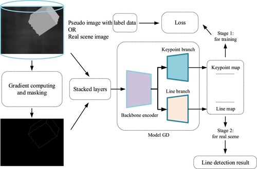
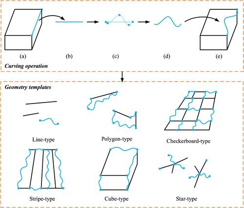
Figure 2. Geometry templates for automatic generation of the curved-line detection dataset.

2.1.1. Pseudo image generation

First, several types of geometry templates were designed in advance for random pseudo-image generation to simulate the different patterns, distributions, and aggregation levels of geometric elements within real-scene images. For example, as Figure 2 shows, line-type, and stripe-type templates represent lines with prominent lengths. Star-type and checkerboard-type templates cover cases where lines are relatively concentrated with more junctions than the former. In addition, random affine transformation was performed over the geometries so that their sizes and densities were randomized in pseudo images to ensure the robustness of the GD model for real scenes. The ability of GD to detect curved lines was trained by randomly selecting straight lines from a geometry template that was then replaced by curved lines. Figure 2 shows the curving operation procedure performed on a straight line based on Lagrange interpolation. The keypoints determining the shape of the curved line are placed at random. Note that the points sampled along the curved line are chosen as the keypoint labels (Figure 3), and there are gaps with a length of 4 pixels in the straight-line state (Figure 2(b)). Notably, the supervision of junctions (i.e. endpoints of lines) and sampled points are weighted, i.e. all pixels in a $3\times 3$ matrix which belongs to a junction, are labeled as 1, while the sampled points are marked based on their pixel coordinates (see Figure 3 and Appendix A).

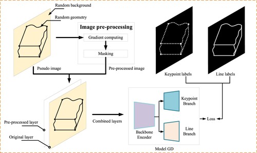
Figure 3. Image pre-processing for model training of GD.

Lastly, the strategy in SuperPoint (DeTone, Malisiewicz, and Rabinovich 2018) was adopted to generate random backgrounds for pseudo images (Figure 3). Gaussian blurring was also applied to the generated images to enhance the ability of GD to detect lines. Randomly generated images only containing Gaussian noise were evenly inserted into the created dataset so that GD could achieve maximal resistance to noise within real images.

2.1.2. Image pre-processing

For better training and faster convergence, image pre-processing was performed on the generated pseudo images described in Section 2.1.1 before the training step shown in Figure 1. Figure 3 shows the two-step procedure of image pre-processing for model training, which includes gradient computing and masking. Specifically, gradient computing provides coarse edge priors for the initial stage of model training, which can be considered tips that accelerate the training process. Masking is an operation that displaces parts of the pixels with zero values after gradient computing. The details of the image pre-processing algorithm are as follows.

First, the Sobel (Cristina and Holban 2013) and Laplacian operators are jointly adopted for image gradient computing. The two employed Sobel masks are: (1) $s_v=\left[\begin{array}{ccc}-1& 0& 1\\ -2& 0& 2\\ -1& 0& 1\end{array}\right]and{s}_h=\left[\begin{array}{ccc}-1& -2& -1\\ 0& 0& 0\\ 1& 2& 1\end{array}\right]$(1) where $s_v$ and $s_h$ respectively correspond to the image gradient in the vertical and horizontal directions, and the two Laplacian masks are denoted by: (2) $l_1=\left[\begin{array}{ccc}0& 1& 0\\ 1& -4& 1\\ 0& 1& 0\end{array}\right]and{l}_2=\left[\begin{array}{ccc}2& 0& 2\\ 0& -8& 0\\ 2& 0& 2\end{array}\right]$(2) The receptive field for each image coordinate $\left(x,y\right)$ is defined in advance as a $3\times 3$ pixel mask denoted by: (3) $f\left(x,y\right)=\left[\begin{array}{ccc}{I}_{x-1,y-1}& I_{x,y-1}& I_{x+1,y-1}\\ I_{x-1,y}& I_{x,y}& I_{x+1,y}\\ I_{x-1,y+1}& I_{x,y+1}& I_{x+1,y+1}\end{array}\right],$(3) where $I_{x,y}\in \left[0,255\right]$ refers to the pixel value of coordinate $\left(x,y\right)$ of image $I$.

To accomplish multi-operator gradient computing, the first operation on the image with respect to the Sobel operator is given as: (4) $G_s\left(x,y\right)=0.5\times \left|f\left(x,y\right)\times s_v\right|+0.5\times \left|f\left(x,y\right)\times s_h\right|.$(4) The second operation is processed using the Laplacian operator and is given by: (5) $G_l\left(x,y\right)=\left|f\left(x,y\right)\times l_1+f\left(x,y\right)\times l_2\right|.$(5) Lastly, the result of image gradient computing is derived by: (6) $G_{s+l}\left(x,y\right)=0.5\times G_s\left(x,y\right)+0.5\times G_l\left(x,y\right).$(6) Second, in the masking step, the regularity of the pixels selected to be displaced by zero values is defined by Equation (7), where $m_{x,y}$ represents whether the image coordinate $\left(x,y\right)$ needs to be masked or not. (7) $m_{x,y}=\{\begin{array}{c}0,y\text{\%}3=0andx\text{\%}3=0\\ 1,y\text{\%}3\ne 0orx\text{\%}3\ne 0\end{array}$(7)

Finally, the pre-processed layer shown in Figure 3 is derived using the following equation: (8) $I_{s+l+m}\left(x,y\right)=m_{x,y}\times G_{s+l}\left(x,y\right).$(8) The input data $X$ for GD training (Figure 3) is constructed by: (9) $X=\left[I\left|\right|I_{s+l+m}\right],$(9) where $\left[\left|\right|\right]$ denotes the layer concatenation operation.

Referring to Equation (6), gradient computing activates the image areas occupied by the edges of geometries and outputs the feature map $G_{s+l}$. The masking operation based on Equations (7) and (8) therefore enriches the textures of the activated areas in $G_{s+l}$, while the inactivated areas without edge gradients tend to remain unchanged. This further enlarges the difference between areas with and without geometric features and benefits model training.

2.1.3. Model inference and training

In the GD training process, the pre-processed two-layer image $X$ (Section 2.1.2) with spatial resolution $h\times w$ is taken as input of the backbone encoder, which is connected with a keypoint and line decoder that outputs the predicted keypoint map $H{P}^c$ and line map $HL$, respectively (Figure 3). Note that $H{P}^c$ is a ${\displaystyle \frac{h}{8}\times {\displaystyle \frac{w}{8}\times 65}}$ feature map where the 1st to 64th channels of a coordinate correspond to the relevant $8\times 8$ patch. The last channel indicates the non-existence of keypoints, obeying a similar strategy to SOLD² (Pautrat et al. 2021) for the keypoint branch. The resolution of the output line map $HL$ is $h\times w$, or the same as $X$.

The network structure of the backbone encoder, keypoint branch, and line branch (see Figure 3) were directly borrowed from SOLD² (Pautrat et al. 2021) to validate the practicability of the proposed self-supervised training scheme for line detection including straight or curved lines. Specifically, the backbone encoder is the same stacked hourglass network proposed in (Newell, Yang, and Deng 2016), outputting a ${\displaystyle \frac{h}{4}\times {\displaystyle \frac{w}{4}\times 256}}$ feature map. The keypoint branch, referring to the junction branch in SOLD², consists of a $3\times 3$ convolution layer followed by a $1\times 1$ convolution layer with 65 channels that outputs $H{P}^c$ with a size of ${\displaystyle \frac{h}{8}\times {\displaystyle \frac{w}{8}\times 65}}$. Finally, the line branch is composed of two consecutive blocks with both containing a $3\times 3$ convolution layer followed by the batch normalization computation, ReLU, and a $\times 2$ subpixel shuffle (Shi et al. 2016). The final operation of the line branch is performed by a $1\times 1$ convolution layer with 1 channel followed by sigmoid activation to derive the line map $HL$ with size $h\times w$.

As illustrated in Figure 3, GD is trained with supervision from keypoint and line labels using the loss functions defined by Equations (10) and (11), respectively: (10) ${\mathcal{L}}_p={\displaystyle \frac{1}{{\displaystyle \frac{h}{8}\times {\displaystyle \frac{w}{8}}}}\sum _{i,j=1}^{{\displaystyle \frac{h}{8},{\displaystyle \frac{w}{8}}}}-\log \left({\displaystyle \frac{\exp \left(H{P}_{i,j,y_{i,j}}^c\right)}{{\sum }_{k=1}^{65}\exp \left(H{P}_{i,j,k}^c\right)}}\right),y_{i,j}\in \left\{1,\dots ,65\right\},}$(10) (11) ${\mathcal{L}}_{line}={\displaystyle \frac{1}{h\times w}\sum _{i,j=1}^{h,w}-H{L}_{i,j}^{GT}\log \left(H{L}_{i,j}\right).}$(11) Note that $y\in \{1,\dots ,65{\}}^{\frac{h}{8}\times \frac{w}{8}}$ (Equation (10)) denotes the ground truth indices for the keypoint position in each patch and $H{P}_{i,j,y_{i,j}}^c\in \{0,1{\}}^{\frac{h}{8}\times \frac{w}{8}\times 65}$ is the related label data for the keypoint map. $H{L}^{GT}\in \{0,1{\}}^{h\times w}$ in Equation (11) represents the ground truth line map.

Finally, a multi-task learning approach proposed by Cipolla, Gal, and Kendall (2018) was adopted for jointly training the two branches, within which dynamic parameters $w_p$ and $w_l$ were optimized during the training process to adaptively weigh the losses ${\mathcal{L}}_p$ and ${\mathcal{L}}_{line}$. The overall objective thus becomes: (12) $\mathcal{L}=e^{-w_p}{\mathcal{L}}_p+e^{-w_l}{\mathcal{L}}_{line}+w_p+w_l$(12)

2.2. GPU-based line vectoring and filtering

As discussed in Section 2.1.3, the straight or curved lines detected from a source image using the trained GD are output as a keypoint and line map (Figure 3), which respectively provide the positions and adjacent relationships of keypoints. In this work, it is necessary to retain stable geometric features (e.g. building contours) and exclude trivial lines (e.g. ripples in lakes) to generate quality geometric priors and accomplish accurate feature matching for high-resolution UAV imagery. Hence, the line detection results need to be converted from raster to vector format so that efficient morphology analysis such as line-length computation can be easily conducted to filter out trivial lines when the GPU memory is limited.

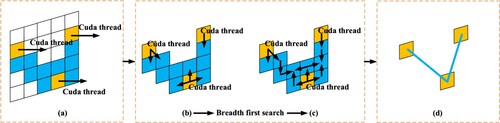
A novel GPU parallel algorithm was developed based on CUDA to achieve high-performance vectorization from UAV imagery with dense predicted keypoints. Figure 4 illustrates the procedure for the vectoring algorithm. First, each predicted keypoint is allocated to an individual CUDA thread for further processing. Second, during CUDA runtime, each CUDA thread simultaneously performs a breadth first search along the paths provided by the predicted line map until it meets another CUDA thread. The thread index is recorded by the traversed coordinate in each step. Finally, the adjacent relationship between a keypoint pair can be easily constructed if the two indices recorded in the neighboring coordinates are different.

Figure 4. GPU parallel algorithm for vectoring: (a) initial stage; (b) – (c) breadth first search stage; and (d) linking stage. The yellow grids represent the keypoints extracted from the output keypoint map, and the blue grids represent the paths derived from the output line map for the breadth first search.

As important as these are, the output keypoint map $H{P}^c$ is first translated to $HP\in {\mathbb{R}}^{h\times w}$ to establish prerequisites for the vectoring algorithm. Keypoint candidates are filtered from $HP$ using an activation threshold ${\xi }_p$, and the final keypoints are derived through the non-maximum suppression of $HP$ using a specific distance constraint of $ϵ=8$ pixels. Finally, paths for the breadth first search (Figure 4(b) and (c)) are extracted from the output line map by a specific activation threshold ${\xi }_l$.

3. Feature matching with geometric priors

The feature matching problem for a UAV image pair can be viewed as the process of matching a pair of graphs since there is a flexible spatial distribution of keypoints and the final matched keypoint pairs satisfy a certain projection relationship. Hence, the GNN technique is adapted for such problems and the data structure considers keypoints as nodes and models keypoint relations as edges.

Motivation. A novel feature-matching method named GeoGlue is proposed in this paper to achieve precise feature matching for UAV imagery. The method combines both SuperGlue (Sarlin et al. 2020) and self-supervised geometric priors (Section 2). In the first part, SuperGlue realizes feature matching in a human fashion that distinguishes salient keypoints for matching based on spatial contextual cues that are integrated from the visual and distributional patterns of co-visible keypoints. Additionally, a GNN structure with stacked self – and cross-attention layers is utilized for processing iterative node aggregation to encode contextual clues into the node descriptors for enhancing keypoint discrimination. Second, geometric priors provided by the self-supervised model GD (Section 2) are employed to perform keypoint proposal, which is more meticulous and comprehensive than the original SuperGlue method built on SuperPoint (DeTone, Malisiewicz, and Rabinovich 2018). Moreover, adequate adjacent candidates can be used for fine-tuning since the keypoints extracted from geometric priors are uniformly distributed on whole bodies of detected lines, which is instrumental in optimal feature matching. Furthermore, keypoint candidates with prominent geometric properties are also advantageous for building spatial context awareness to encode distinctive descriptors for matching.

Feature reasoning. The architecture for feature reasoning with GD and SuperGlue, including keypoint generation and description, can be seen in Figure 5. For feature matching, a specific case is that the two images to be matched (i.e. image $Q$ and image $S$) are processed as inputs into GD and SuperPoint. The two output keypoint groups from the two models are combined as one set for each image. The former focuses on meticulous geometry extraction while the latter provides balanced attention to the whole image. The image coordinates of the keypoints are represented by $p=\{\left(x_i,y_i\right)\in h\times w{\}}_{i=1}^n$ where $n$ denotes the total number of keypoints from images $Q$ or $S$. In the further computation of keypoint descriptors based on GAT, the confidence values $c=\{c_i\in \mathbb{R}{\}}_{i=1}^n$ and initial visual descriptors $d=\{d_i\in {\mathbb{R}}^D{\}}_{i=1}^n$ of keypoints are sampled from the feature maps produced by SuperPoint (DeTone, Malisiewicz, and Rabinovich 2018) in accordance with positions $p$. Then, to obtain the initial node state ${\phi }_i^{\left(0\right)}$of keypoint $i$. 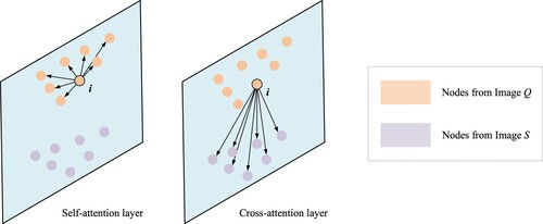This enables feature integration for the keypoint’s appearance, location, and certainty, as shown in Equation (13): (13) ${\phi }_i^{\left(0\right)}=d_i+ML{P}_{KP}\left(p_i\left|\right|c_i\right),$(13) where $\left|\right|$ denotes concatenation of two vectors. After node state initialization, these embeddings are taken as input for a stack of self – and cross-attention layers, as shown in Figure 5. Specifically, the data processed above can be considered a graph where the nodes represent the keypoints from images $Q$ and $S$ and the edges reflect their associations. As for the self-attention layer, each node ($i$) is connected with all other nodes in the same image. Conversely, each of the nodes in the cross-attention layer is connected with all of the nodes within the other image (Figure 6). The graph reasoning aspect of GAT is composed of stacked self – and cross-attention layers that are repeated $L$ times (Figure 5), which iteratively performs information aggregation (Equation 14) among the linked nodes to encode contextual clues (e.g. the pattern of local distribution and visual information from neighbors) into the node descriptors. The mathematical principle for graph reasoning is as follows.

Figure 5. The architecture of feature reasoning, including the generation and description of keypoints with GD and SuperGlue, which is composed of SuperPoint and a graph attention network (GAT). Note that the symbols (Op I) and (Op II) denote the operation $\left|\right|$ and the sum operation in Equation (13), respectively.

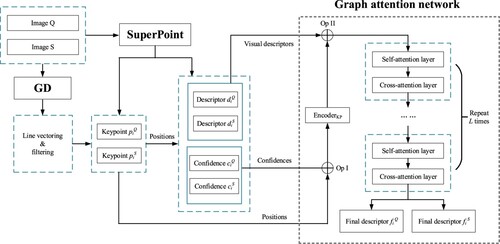
Figure 6. Connection patterns of node $i$ in the self-attention and cross-attention layers.

To update the node embeddings, another MLP named $\mathrm{M}\mathrm{L}{\mathrm{P}}_{\mathrm{M}\mathrm{s}\mathrm{g}}$ is utilized for fusing the immediate embeddings ${\phi }^{\left(l-1\right)}$ and messages $\{m_{A\to i}{\}}_{i=1}^n$ into new encodings through vector concatenation, where $A=\left\{\left(i,j\right)\in \left\{1,\dots ,n\right\}\times \left\{1,\dots ,n\right\}\right\}$ represents the edges among nodes. The graph reasoning process of the self – or cross-attention layer $l$ is summarized by Equation (14): (14) ${\phi }_i^{\left(l\right)}={\phi }_i^{\left(l-1\right)}+\mathrm{M}\mathrm{L}{\mathrm{P}}_{\mathrm{M}\mathrm{s}\mathrm{g}}\left(\left[{\phi }_i^{\left(l-1\right)}\left|\right|m_{A\to i}^{\left(l-1\right)}\right]\right).$(14) Messages $\{m_{A\to i}{\}}_{i=1}^n$ are high-dimensional vectors for each node that are aggregated from the neighbors of each node. For neighbor information retrieval, the embeddings of node $i$ and its neighbor node $j$ are first transformed into vectors $q_i$, $k_j$, and $v_j$ through linear projection (Sarlin et al. 2020), as shown by Equations (15) and (16): (15) $q_i^{\left(l\right)}=W_1^{\left(l\right)}{\phi }_i^{\left(l-1\right)}+b_1^{\left(l\right)},$(15) (16) $\left[\begin{array}{c}{k}_j^{\left(l\right)}\\ v_j^{\left(l\right)}\end{array}\right]=\left[\begin{array}{c}{W}_2^{\left(l\right)}\\ W_3^{\left(l\right)}\end{array}\right]{\phi }_j^{\left(l-1\right)}+\left[\begin{array}{c}{b}_2^{\left(l\right)}\\ b_3^{\left(l\right)}\end{array}\right].$(16) Then, messages $\{m_{A\to i}{\}}_{i=1}^n$ are therefore derived with a weighted sum method illustrated by Equation (17): (17) $m_{A\to i}=\sum _{j:\left(i,j\right)\in A}{\alpha }_{ij}{v}_j,$(17) where $\{{\alpha }_{ij}{\}}_{j:\left(i,j\right)\in A}$ denotes the attention weights allocated by the softmax function based on similarities among node $i$ and its neighbors (Equation (18)). (18) ${\alpha }_{ij}=\mathrm{S}\mathrm{o}\mathrm{f}\mathrm{t}\mathrm{m}\mathrm{a}{\mathrm{x}}_{\mathrm{j}}\left(q_i^T{k}_j\right)$(18) Lastly, the reasoning results ${\phi }^{\left(L\right)}$ are output by the $L^{th}$ layer after $L$ iterations of information diffusion across the self – and cross-attention graphs, and the ultimate node descriptors $\{f_i{\}}_{i=1}^n$ are obtained by linear projection: (19) $f_i=W_4^{\left(L\right)}{\phi }_i^{\left(L\right)}+b_4^{\left(L\right)}$(19)

Keypoint matching. Under the condition that the final descriptors of keypoints are given within images $Q$ and $S$, the Sinkhorn algorithm is then employed to solve the keypoint matching problem as an optimal transport problem (Sinkhorn and Knopp 1967). The algorithm is differentiable and enables end-to-end training as described in SuperGlue (Sarlin et al. 2020) in order to derive an optimized feature matching ability. The algorithm is articulated as follows.

Supposing that the keypoint numbers of images $Q$ and $S$ are $n_Q$ and $n_S$, respectively, a matrix $M\in {\mathbb{R}}^{n_Q\times n_S}$, which stores the similarity score of each candidate pair $\left(i,j\right)\in n_Q\times n_S$, is first computed by: (20) $M_{i,j}=〈f_i^Q,f_j^S〉,\mathrm{\forall }\left(i,j\right)\in n_Q\times n_S,$(20) where $〈\cdot ,\cdot 〉$ denotes the inner product. If there are unmatched keypoints, an augmented score matrix $\overline{M}\in {\mathbb{R}}^{\left(n_Q+1\right)\times \left(n_S+1\right)}$ is set up from $M$ by adding a new row and column filled with a learnable parameter (Sarlin et al. 2020). Then, a probability matrix $P\in [0,1{]}^{\left(n_Q+1\right)\times \left(n_S+1\right)}$ is defined to be the objective indicating the final matching results, and the primary matrix $P$ is considered an assignment matrix that is optimized for maximizing the transmission value (i.e. $\sum _{i,j}{\overline{M}}_{i,j}{P}_{i,j}$) under the two constraints with respect to the marginal probabilities: (21) $P\ast 1_{n_S+1}=[1_{n_Q}^T,n_S{]}^{T}and{P}^T\ast 1_{n_Q+1}=[1_{n_S}^T,n_Q{]}^T.$(21) Finally, the optimized $P$ can be derived by the fixed-point method for $T$ iterations based on Equations (21) and (22): (22) $p_{ij}={\alpha }_i{e}^{-\lambda {\overline{M}}_{i,j}}{\text{β}}_j,\left(i,j\right)\in n_Q\times n_S,$(22) where $\alpha$ and $\text{β}$ denote the unsolved parameters, and $\lambda$ is set as $-1$ in this study. The parameter $T=20$ was also set in our experiments.

4. Experiments and results

In this study, comprehensive experiments were conducted to verify the effectiveness of self-supervised geometric priors and show the superiority of GeoGlue compared with recent learning-based approaches and traditional mainstream methods such as SIFT (Lowe 2004) and ORB (Rublee et al. 2011) that use nearest-neighbor matching. Four specialized datasets were introduced in Section 4.1. The experiment results are presented in Sections 4.2, 4.2.1, and 4.2.2.

Implementation details. The GD model (Section 2.1) was trained by the auto-generated dataset, or the pseudo image dataset, illustrated in Section 4.1.1. The training process used Adam with a learning rate of 5e-4 and batch size of 2. As described in Section 3, GeoGlue is built upon SuperGlue and the pretrained network provided by Sarlin et al. (2020) was used in the following experiments. All experiments were implemented in PyTorch and OpenCV with an RTX 4000 GPU (8 GB).

4.1. Datasets

4.1.1. Pseudo image dataset

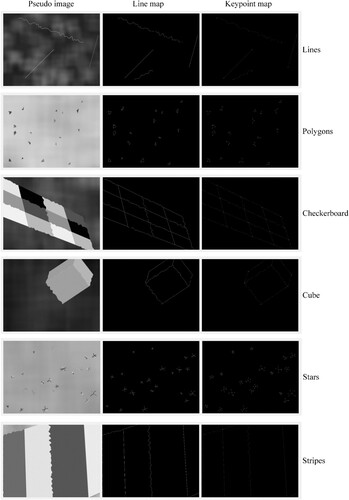
In accordance with Sections 2.1.1 and 2.1.2, a pseudo image dataset consisting of rendered images and labels was first created to train the GD model. Table 1 presents the statistical numbers for the training data generated using the six types of geometry templates (i.e. line, polygon, checkerboard, cube, star, and stripe). Notably, as described in Section 2.1.1, the shapes, sizes, and locations of the generated geometry objects were random. Some samples are provided in Appendix A. Finally, 10,000 pseudo images only containing Gaussian noise were evenly inserted into the created dataset to improve noise resistance.

Table 1. Statistical results of various types of geometry templates in the pseudo image dataset.

Geometry template	Line	Polygon	Checkerboard	Cube	Star	Stripe
Number	10000	30000	20000	10000	20000	20000

4.1.2. Benchmark datasets

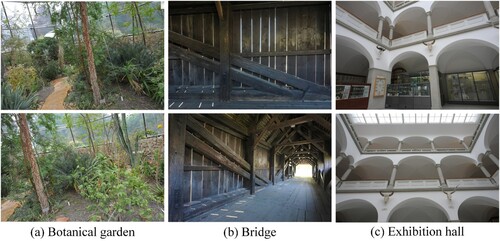
Two benchmark datasets named Tanks & Temples (Knapitsch et al. 2017) and ETH3D (Schöps et al. 2017) were utilized for pose estimation experiments. These two datasets both consist of images captured under strong viewpoint variations. In the Tanks & Temples dataset, four challenging scenes (auditorium, ballroom, lighthouse, and temple) containing rich regions with repetitive patterns were selected to evaluate robustness. Additionally, ETH3D featured stronger light changes and sparser views in comparison to Tank & Temples, and three difficult scenes (botanical garden, bridge, and exhibition hall) were chosen for experiments. Some examples of the image pairs provided by Tank & Temples and ETH3D are displayed in Figures 7 and 8. The two types of datasets used in the experiments are available at https://figshare.com/ndownloader/files/38945210.

Figure 7. Examples of image pairs from Tanks & Temples.

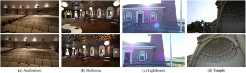
Figure 8. Examples of image pairs from ETH3D.

4.1.3. High-resolution UAV image dataset

High-resolution UAV imagery covering diverse scenes were collected and used to fully test the feature matching and generalization of GeoGlue. The high-resolution UAV image dataset contains four types of aerial images, including: (a) city scenes with large features (e.g. tall buildings) (City A), (b) city scenes with small-sized features (e.g. sculptures) (City B), (c) village scenes, and (d) nature scenes (e.g. forests and lakes). Images in the dataset were organized as image pairs in view of their overlap rates, and a resolution of $H_I=4000$ (height) and $W_I=6000$ (width). The counts of different scenes are listed in Table 2. Some specific samples are shown in Figure 9, and the whole dataset can be directly downloaded at https://figshare.com/ndownloader/files/38095920.

Figure 9. High-resolution UAV image dataset used for feature matching experiments (Section 4.1.2).

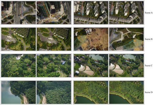
Table 2. Statistics of the four types of scenes in the high-resolution UAV dataset.

Scene	City A	City B	Village	Nature
Image pair number	185	123	45	22

4.2. Validation of self-supervised geometric priors

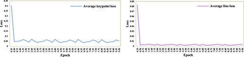
The GD model was first trained using the pseudo image dataset (Section 4.1.1). Figure 10 presents the training curves for the average losses in the keypoint and line maps (Section 2.1.3) across every 0.25 epoch. The losses stabilized at around 0.04 and 0.01 after 2 epochs, which demonstrates the learning ability of the geometric prior extraction task. In this paper, we chose a model that was trained after 8 epochs, consuming 52 h, as the GD for the following experiments. The activation thresholds were set as ${\xi }_p={\displaystyle \frac{6}{255}}$ and ${\xi }_l={\displaystyle \frac{40}{255}}$ for the line vectoring and filtering processes described in Section 2.2.

Figure 10. Training curves for the GD model.

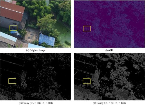
Figure 11 shows the comparative results from line detection with GD and Canny (Canny 1986), where parameters $T_1$ and $T_2$ denote the gradient thresholds used for the Canny algorithm. Although Canny proved to be effective in line detection, some defects, e.g. missing lines (see the yellow boxes in Figure 11), were found to still exist due to the complexity of textures and shading displayed in high-resolution UAV imagery. In comparison, GD can achieve more acceptable results, while trivial lines can be disregarded using the line-length filtering process described in Section 2.2.

Figure 11. Comparison of line detection results produced by GD and Canny.

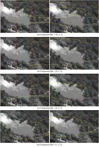
As described in Section 3 and displayed in Figure 11, the keypoints detected by GD were primarily distributed along lines, providing quality candidates for feature matching. We visualized the keypoint descriptor produced by GeoGlue using PCA (Section 3). This was carried out to illustrate the feasibility of performing feature matching given the condition that adjacent keypoints were inclined to be homogeneous in terms of location and visual features. As shown in Figure 12, adjacent keypoints were distinguishable by their RGB colors derived from the first three components after PCA using a linear transformation. In this sample, it was apparent that more than 6 components were significant in the discrimination of keypoint descriptors according to the resulting eigenvalues (Figure 12). The eigenvalues of the first four components are listed in Table 3. In addition, Appendix B (Figure 21) displays the results of descriptor visualization for a sample image pair under different component combinations while only using the first four components. This result shows the relevance between two specific regions for different images that reflect the same spatial location. Therefore, the feature representation provided by GeoGlue is position-dependent based on the quality keypoint proposed by GD, which helps form rich spatial context information during model inference.

Figure 12. A sample of the eigenvalues of all descriptor components following PCA. The components are sorted by their value size, and the descriptors for the first three components are visualized.

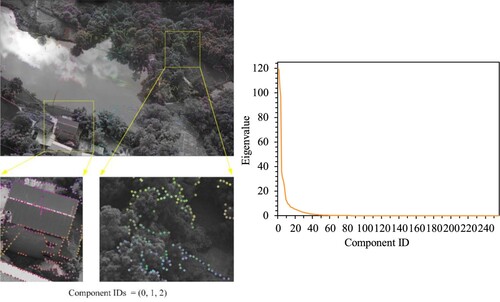
Table 3. Eigenvalues for the first four descriptor components based on PCA.

Component ID	0	1	2	3
Eigenvalue	119.813	118.801	104.513	97.087

4.2.1. Pose estimation evaluated by the benchmark datasets

We conducted pose estimation experiments using the two benchmark datasets described in Section 4.1.2 to quantitatively verify the effectiveness of GeoGlue. GeoGlue was compared with recent learning-based approaches, namely SuperGlue (Sarlin et al. 2020) and LoFTR (Sun et al. 2021), and the traditional mainstream methods of SIFT (Lowe 2004) and ORB (Rublee et al. 2011) with nearest-neighbor matching. Pose estimation includes solving the relative rotation $R$ and translation $T$ between a pair of adjacent frames based on essential matrix decomposition (Hartley 1995) and applying random sample consensus (RANSAC) to exclude outliers. For a fair comparison, all poses derived from diverse methods were aligned to the same scale as the ground truth data by scaling the estimated translation $T$.

The approach to evaluating pose accuracy is described as follows. First, for each frame pair, the percentages of the relative rotation error (using degrees) and translation error (using L2 distance) are calculated from the total rotations and translations of the whole frame pairs of a scene. The number of frame pairs is counted and the computed percentages are placed within a certain threshold. Two thresholds {0.2%, 0.5%} are chosen, and the statistical number of frame pairs are also presented as percentages (i.e. AUC) to intuitively show the stability of diverse methods across the whole trajectory of a scene. In Tables 4 and 5, the ‘max error’ is used to denote the maximum relative pose error among all frame pairs, and the ‘final error’ represents the relative pose error of the last frame against the pose of the first frame.

Table 4. Baseline comparison of pose estimation results for the first fifty frames in Tanks & Temples. The numbers presented in brackets in the ‘rotation error AUC’ and ‘translation error AUC’ columns refer to the specific frame pair number.

Method	Scene	$R$ error AUC [%]$\uparrow$		$T$ error AUC [%]$\uparrow$		Max error [%]$\downarrow$		Final error [%]$\downarrow$
		@0.2%	@0.5%	@0.2%	@0.5%	$R$	$T$	$R$	$T$
SIFT + NN	Auditorium	100 (50)	100 (50)	96.0 (48)	100 (50)	0.142	0.23	0.28	0.41
	Ballroom	82.0 (41)	94.0 (47)	58.0 (29)	76.0 (38)	177.83	2.49	177.29	70.07
	Lighthouse	82.0 (41)	100 (50)	80.0 (40)	96.0 (48)	0.46	0.91	1.32	3.39
	Temple	98.0 (49)	100 (50)	68.0 (34)	88.0 (44)	0.21	1.16	0.40	3.62
ORB + NN	Auditorium	80.0 (40)	92.0 (46)	38.0 (19)	68.0 (34)	2.56	4.34	3.14	5.55
	Ballroom	60.0 (30)	84.0 (42)	14.0 (7)	32.0 (16)	177.86	3.71	128.87	56.95
	Lighthouse	40.0 (20)	68.0 (34)	32.0 (16)	44.0 (22)	3.02	4.59	3.42	16.46
	Temple	62.0 (31)	78.0 (39)	20.0 (10)	48.0 (24)	27.39	7.67	15.81	63.71
SuperGlue	Auditorium	100 (50)	100 (50)	80.0 (40)	98.0 (49)	0.19	0.59	0.48	0.57
	Ballroom	76.0 (38)	94.0 (47)	38.0 (19)	76.0 (38)	177.87	2.71	177.60	43.72
	Lighthouse	62.0 (31)	96.0 (48)	60.0 (30)	92.0 (46)	0.98	1.34	1.41	2.32
	Temple	100 (50)	100 (50)	74.0 (37)	92.0 (46)	0.13	0.88	.0.247	3.52
LoFTR	Auditorium	100 (50)	100 (50)	94.0 (47)	100 (50)	0.138	0.34	0.24	0.73
	Ballroom	90.0 (45)	98.0 (49)	36.0 (18)	80.0 (40)	0.82	2.26	1.85	4.50
	Lighthouse	84.0 (42)	100 (50)	86.0 (43)	98.0 (49)	0.42	0.65	0.47	1.49
	Temple	100 (50)	74.0 (37)	100 (50)	90.0 (45)	0.16	1.11	0.245	2.45
GeoGlue	Auditorium	100 (50)	100 (50)	96.0 (48)	100 (50)	0.11	0.22	0.36	0.56
	Ballroom	82.0 (41)	98.0 (49)	60.0 (30)	90.0 (45)	0.69	0.93	0.93	1.02
	Lighthouse	78.0 (39)	96.0 (48)	66.0 (33)	96.0 (48)	0.65	0.54	0.72	1.14
	Temple	100 (50)	100 (50)	78.0 (39)	100 (50)	0.11	0.49	0.41	1.06

Table 5. Baseline comparison of pose estimation results for the first fifty frames in ETH3D. The numbers presented in brackets in the ‘rotation error AUC’ and ‘translation error AUC’ columns refer to the specific frame pair number.

Method	Scene	$R$ error AUC [%]$\uparrow$		$T$ error AUC [%]$\uparrow$		Max error [%]$\downarrow$		Final error [%]$\downarrow$
		@0.2%	@0.5%	@0.2%	@0.5%	$R$	$T$	$R$	$T$
SIFT + NN	Botanical garden	64.3 (9)	71.4 (10)	42.9 (6)	64.3 (9)	27.17	17.28	19.90	49.29
	Bridge	96.2 (101)	97.1 (102)	96.2 (101)	97.1 (102)	13.79	6.33	20.11	7.81
	Exhibition hall	100 (54)	100 (54)	98.1 (53)	100 (54)	0.12	0.46	0.21	0.57
ORB + NN	Botanical garden	0.0 (0)	0.0 (0)	0.0 (0)	0.0 (0)	74.58	15.17	19.03	89.87
	Bridge	71.4 (75)	79.0 (83)	78.1 (82)	81.9 (86)	26.00	2.98	20.77	5.97
	Exhibition hall	53.7 (29)	81.5 (44)	31.5 (17)	37.0 (20)	16.30	9.57	15.33	20.55
SuperGlue	Botanical garden	71.4 (10)	100 (14)	71.4 (10)	92.9 (13)	0.36	0.68	0.67	2.37
	Bridge	100 (105)	100 (105)	100 (105)	100 (105)	0.19	0.05	0.33	0.24
	Exhibition hall	100 (54)	100 (54)	100 (54)	100 (54)	0.03	0.10	0.144	0.22
LoFTR	Botanical garden	100 (14)	100 (14)	100 (14)	100 (14)	0.08	0.09	0.07	0.18
	Bridge	100 (105)	100 (105)	100 (105)	100 (105)	0.11	0.19	0.10	0.22
	Exhibition hall	100 (54)	100 (54)	100 (54)	100 (54)	0.04	0.15	0.136	0.41
GeoGlue	Botanical garden	100 (14)	100 (14)	100 (14)	100 (14)	0.17	0.19	0.34	0.45
	Bridge	100 (105)	100 (105)	100 (105)	100 (105)	0.07	0.04	0.19	0.06
	Exhibition hall	100 (54)	100 (54)	98.1 (53)	100 (54)	0.07	0.49	0.135	0.63

The quantitative results are shown in Tables 4 and 5. As described in Section 4.1.2, four challenging scenes from Tanks & Temples (Knapitsch et al. 2017) and three difficult scenes from ETH3D (Schöps et al. 2017) were chosen for comparing GeoGlue and other state-of-the-art methods. In comparison with SuperGlue, GeoGlue was found to achieve a prominent improvement in pose estimation robustness and accuracy for almost all scenes in Tanks & Temples and ETH3D. Additionally, GeoGlue showed a more competitive performance for scenes in Tanks & Temples and ETH3D compared with LoFTR.

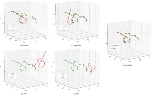
In addition to the tables, Figures 13 and 14 display the qualitative results of the estimated trajectories obtained from diverse methods. The bridge scene in ETH3D was chosen for its great perspective transforms among adjacent frames. The ballroom scene in Tanks & Temples was selected due to the presence of large areas of repetitive patterns, which are even quite difficult for manual registration, as shown in Section 4.1.2. Despite all this, GeoGlue achieved satisfactory stability for pose estimation and showed the best performance compared to baseline methods.

Figure 13. Qualitative results for bridge scene in ETH3D.

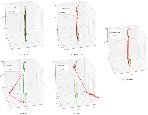
Figure 14. Qualitative results for the ballroom scene in Tanks & Temples.

4.2.2. Feature matching evaluation using the UAV dataset

The reprojection error (RE), computed by Equation (23), was employed to evaluate the feature matching performance in experiments carried out on the high-resolution UAV image dataset: (23) $RE=\left\{\left(R{E}_x,R{E}_y\right)|R{E}_x={\displaystyle \frac{\left|x_{rp}-x_o\right|}{W_I}\times 100\text{\%},R{E}_y={\displaystyle \frac{\left|y_{rp}-y_o\right|}{H_I}\times 100\text{\%}}}\right\}.$(23) Note that, $\left(x_{rp},y_{rp}\right)$ is computed using Equation (24) and represents the reprojection coordinate of a matched keypoint $\left(x_o,y_o\right)$ from a frame. As described in Section 4.1.3, $H_I$ and $W_I$ represent the height and width of a UAV image. In Equation (24), $[X,Y,Z{]}^T$ denotes the normalized 3D coordinate of the keypoint $\left(x_o,y_o\right)$ derived by triangulation under the epipolar geometry model (Zhang 1998) for a pair of adjacent frames. $K$ is the camera intrinsic matrix and $s$ denotes the scale factor. $R$ and $T$ are derived from essential matrix decomposition (Hartley 1995) with RANSAC and represent the relative pose between the frame pair. The estimated pose receives no influence from matches that are viewed as outliers by the RANSAC algorithm. Thus, large reprojection deviations can be produced from the outliers using Equation (23), and RE can reflect the feature-matching performance during evaluation. (24) $s\left[\begin{array}{c}{x}_{rp}\\ y_{rp}\\ 1\end{array}\right]=K\left(R\left[\begin{array}{c}X\\ Y\\ Z\end{array}\right]+T\right)$(24) Since the GPU memory is limited, the input UAV image is inevitably resized before model inference. Coincidentally, image partitioning and sub-image matching are preparatory steps for dense matching, which is instrumental for 3D reconstruction with high-resolution UAV images and dependent on the results of global matching. Therefore, it is important to conduct the following feature matching (i.e. global matching) experiments using RE (Equation (23)), which can simultaneously reflect the deviations of matches in the horizontal and vertical directions. The results are tightly correlated with the model performance for feature-matching.

As discussed above, the height and width of the input UAV image was resized to $2000\times 3000$ (a quarter of the original size $H_I\times W_I$) for the extraction of self-supervised geometric priors using GD. Additionally, it was easy to calculate the line lengths since the adjacent relationships among the extracted keypoints were already derived by line vectoring (Figure 5). The line lengths can then be used to filter out trivial lines. In this study, the line-length threshold was dynamically adjusted to satisfy an upper limit keypoint number (${\xi }_u=10000$) due to GPU memory limitation.

Table 6 presents the comparative outcomes between SuperGlue and GeoGlue for various scenes in the high-resolution UAV image dataset. For GeoGlue, we particularly compare the matching results from the keypoints derived by SuperPoint (see Figure 5). The number of matched keypoints was observed to increase with the aid of geometric priors from GD because more high-quality candidates were offered for matching. In addition, the results for the mean, standard deviation, and maximum values simultaneously declined compared to those of SuperGlue, demonstrating the power of the keypoints proposed by GD.

Table 6. RE for the four types of scenes in the high-resolution UAV dataset. GeoGlue (S) only refers to the keypoint matches from SuperPoint (i.e. the same keypoint proposal results as SuperGlue).

Object	Scene	Number	MEAN RE$\downarrow$	STD RE$\downarrow$	MAX RE$\downarrow$
SuperGlue	City A	532	(0.029%, 0.221%)	(0.038, 0.278)	(0.218%, 1.418%)
	City B	562	(0.037%, 0.176%)	(0.053, 0.249)	(0.298%, 1.391%)
	Village	525	(0.029%, 0.206%)	(0.042, 0.281)	(0.284%, 1.567%)
	Nature	481	(0.002%, 0.195%)	(0.003, 0.306)	(0.017%, 2.124%)
GeoGlue (S)	City A	548	(0.019%, 0.155%)	(0.027, 0.228)	(0.161%, 1.259%)
	City B	585	(0.021%, 0.097%)	(0.033, 0.160)	(0.241%, 1.243%)
	Village	557	(0.017%, 0.127%)	(0.031, 0.225)	(0.224%, 1.383%)
	Nature	555	(0.004%, 0.134%)	(0.007, 0.206)	(0.055%, 1.437%)
GeoGlue	City A	4404	(0.012%, 0.100%)	(0.019, 0.159)	(0.188%, 1.445%)
	City B	4485	(0.023%, 0.106%)	(0.033, 0.154)	(0.445%, 1.899%)
	Village	3595	(0.019%, 0.141%)	(0.031, 0.216)	(0.299%, 1.951%)
	Nature	4373	(0.005%, 0.173%)	(0.007, 0.235)	(0.073%, 1.915%)

Moreover, in terms of the results for all keypoints in GeoGlue, the mean value and standard deviation of RE were both better than those of SuperGlue. This result validates the rationality and feasibility of self-supervised geometric priors since the keypoints from GD were the primary candidates used for matching. The extreme cases of max RE shown in the last column in Table 6 indicate that the maximum reprojection deviations (Equation (23)) resulting from GeoGlue were reasonable and close to those of SuperGlue.

Comparative experiments were performed using recent learning-based approaches such as SuperGlue (Sarlin et al. 2020) and LoFTR (Sun et al. 2021) as well as traditional mainstream methods such as SIFT (Lowe 2004) with nearest-neighbor matching. LoFTR, which infers based on Transformer (Vaswani et al. 2017), has been demonstrated as an excellent approach for producing abundant high-quality matches. Image pairs with small overlapping regions were employed in experiments to test the performance of the above methods.

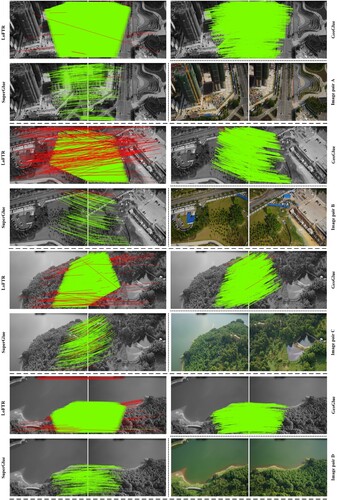
Figure 15 shows the matching quality of LoFTR, SuperGlue, and GeoGlue for various scenes, using image pairs with small overlapping regions. In the case of LoFTR, the matching candidates were evenly distributed across image pairs and produce more matches but $R{E}^{\mathrm{\prime }}s\ge 2\text{\%}$ occurred frequently with large deviations. In comparison, GeoGlue offered more matches than SuperGlue while retaining matching quality and provided more satisfactory results for less extreme deviation cases than LoFTR.

Figure 15. Qualitative results of feature matching from diverse methods using the image pairs of various scenes with small overlapping regions, where the red lines represent the matches with $RE\ge 2\text{\%}$ in the horizontal or vertical directions.

Table 7 presents the quantitative results for feature matching using the above methods. GeoGlue generally outperformed the other methods and featured better performance stability with small maximum REs and less extreme cases of large RE values (i.e. $RE\ge 2\text{\%}$) for diverse scenes. This result verifies the robustness and practicality of GeoGlue for feature matching using high-resolution UAV imagery. Moreover, as observed in Table 7, the number of matches provided by GeoGlue was reasonable and the statistical results for RE were acceptable, demonstrating the suitability of GeoGlue for global matching tasks. Lastly, the robustness of GeoGlue was evaluated using the entire UAV image dataset. The statistical results listed in Table 8 show that GeoGlue achieved stable performance in various scenes.

Table 7. Reprojection error results for the four types of scenes using image pairs with small overlapping regions. The last four columns provide the percentage of matches, and the REs are in the relevant numerical intervals. Note that the symbol ‘·’ is a placeholder for the data row with a matching failure.

Method	Scene	Number	MAX RE$\downarrow$	$RE\in \left[0,1\text{\%}\right)\uparrow$	$RE\in \left[1\text{\%},2\text{\%}\right)$	$RE\ge 2\text{\%}\downarrow$
SIFT + NN	City A	8606	(22.35%, 63.89%)	(76.17%, 52.68%)	(7.77%, 1.63%)	(16.06%, 45.69%)
	City B	8886	(8.43%, 61.03%)	(96.04%, 89.23%)	(1.76%, 0.48%)	(2.21%, 10.29%)
	Village	17778	(15.76%, 59.99%)	(72.70%, 50.75%)	(13.04%, 2.06%)	(14.25%, 47.19%)
	Nature	8928	(>100%, > 100%)	(81.97%, 82.15%)	(0.13%, 0.44%)	(17.90%, 17.42%)
SuperGlue	City A	110	(5.04%, 1.20%)	(80.0%, 98.18%)	(15.45%, 1.82%)	(4.55%, 0%)
	City B	160	(2.79%, 0.60%)	(90.62%, 100%)	(8.75%, 0%)	(0.63%, 0%)
	Village	0	(·%, ·%)	(·%,·%)	(·%,·%)	(·%,·%)
	Nature	211	(0.27%, 2.15%)	(100.0%, 93.36%)	(0%, 6.16%)	(0%, 0.47%)
LoFTR	City A	3209	(>100%, > 100%)	(95.23%, 95.48%)	(0.03%, 0.22%)	(4.74%, 4.30%)
	City B	3248	(>100%, > 100%)	(95.04%, 95.32%)	(0.06%, 0.06%)	(4.90%, 4.62%)
	Village	5792	(2.98%, 27.69%)	(99.12%, 97.81%)	(0.71%, 0.16%)	(0.17%, 2.04%)
	Nature	1438	(>100%, > 100%)	(84.21%, 85.95%)	(0.35%, 1.39%)	(15.44%, 12.66%)
GeoGlue	City A	551	(1.74%, 0.41%)	(97.64%, 100%)	(2.36%, 0%)	(0%, 0%)
	City B	1274	(3.27%, 0.66%)	(96.86%, 100%)	(2.59%, 0%)	(0.55%, 0%)
	Village	420	(0.67%, 5.89%)	(100%, 88.10%)	(0%, 5.24%)	(0%, 6.67%)
	Nature	851	(10.23%, 4.13%)	(86.25%, 95.53%)	(6.93%, 3.29%)	(6.82%, 1.18%)

Table 8. Statistical results for feature matching produced by GeoGlue with respect to the whole UAV image dataset. The columns ranging from the second onward present the numbers and percentages of image pairs. And the title bar shows the numerical intervals for the percentage of matches whose $RE\ge 2\text{\%}$ from an image pair, denoted by $ECs$.

Scene	$ECs\in \left[0,1\text{\%}\right)$	$ECs\in \left[1\text{\%},3\text{\%}\right)$	$ECs\in \left[3\text{\%},7\text{\%}\right)$	$ECs\ge 7\text{\%}$
City A	185 (100.0%)	0 (0.0%)	0 (0.0%)	0 (0.0%)
City B	123 (100.0%)	0 (0.0%)	0 (0.0%)	0 (0.0%)
Village	44 (97.78%)	0 (0.0%)	1 (2.22%)	0 (0.0%)
Nature	21 (95.45%)	0 (0.0%)	1 (4.55%)	0 (0.0%)

4.2.3. Time performance and GPU memory cost

Tables 9, 10, and 11 respectively display the time performance and maximum GPU memory consumption in the feature matching step by GeoGlue for the Tanks & Temples, ETH3D, and the high-resolution UAV datasets. The table includes the average time for line detection ($A{T}_{LD}$) on a frame pair, the average time for the whole matching step including line detection and feature matching ($A{T}_{Wh}$), and the total time ($T{T}_{Wh}$).

Table 9. Time performance and maximum GPU memory cost in the feature matching step produced by GeoGlue and Tanks & Temples.

Scene	Frame pairs	Image size (H*W)	$A{T}_{LD}$ (s)	$A{T}_{Wh}$ (s)	$T{T}_{Wh}$ (s)	Max GPU memory (GB)
Auditorium	50	648*1152	0.78	2.13	106.36	4.3GB
Ballroom	50	648*1152	1.20	3.80	190.09	5.1GB
Lighthouse	50	648*1152	0.63	1.77	88.34	5.1GB
Temple	50	648*1152	0.88	2.77	138.57	5.1GB

Table 10. Time performance and maximum GPU memory cost in the feature matching step produced by GeoGlue and ETH3D.

Scene	Frame pairs	Image size (H*W)	$A{T}_{LD}$ (s)	$A{T}_{Wh}$ (s)	$T{T}_{Wh}$ (s)	Max GPU memory (GB)
Botanical garden	14	1032*1552	1.96	5.78	80.98	5.5GB
Bridge	105	1032*1552	1.80	5.56	584.32	5.9GB
Exhibition hall	54	1032*1552	1.80	5.57	300.74	5.9GB

Table 11. Time performance and maximum GPU memory cost of feature matching produced by GeoGlue and the high-resolution UAV dataset.

Scene	Frame pairs	Image size (H*W)	$A{T}_{LD}$ (s)	$A{T}_{Wh}$ (s)	$T{T}_{Wh}$ (s)	Max GPU memory (GB)
City A	185	2000*3000	3.10	6.20	1146.15	7.5GB
City B	123	2000*3000	2.95	6.13	753.95	7.5GB
Village	45	2000*3000	2.89	6.03	271.21	7.5GB
Nature	22	2000*3000	2.94	6.13	134.94	7.5GB

As discussed in Sections 2 and 3, most of the computational resource requirements were from line detection and feature matching procedures. Thus, the resolution of input images and the richness of geometric features in the corresponding scene were the primary factors affecting the time performance and GPU memory cost. From the tables, it can be seen that GeoGlue cannot achieve real-time processing, and the average processing time for each frame pair is several seconds. In addition, the GPU memory cost is around 5 GB for Tanks & Temples and ETH3D, and 7.5 GB for the UAV dataset, which is caused by the expensive computation of the Sinkhorn algorithm used for keypoint matching (Section 3).

4.3. 3d reconstruction and remaining issues

As illustrated in Sections 4.2.1 and 4.2.2, GeoGlue shows superiority in feature matching since it is robust and effective to various scenes. As described in Section 4.2.2, global matching is the prerequisite for image partitioning and sub-image matching for high-resolution UAV imagery, which aims at fine-grained matching for subsequent 3D reconstruction. Therefore, the process includes the following steps. First, regularly divide the query image into $4\times 4$ sub-images (like Figure 16). Second, compute the relevant image blocks within the target image for each sub-image of the query image by averaging the deviations of matches from global matching (see Figure 16). Lastly, perform feature matching between each sub-image pair.

Figure 16. Samples of fine-grained matching with GeoGlue.

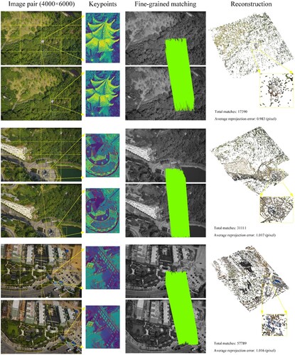
Figure 16 shows some samples of the results from fine-grained matching with GeoGlue. The current method can achieve effective results for 3D reconstruction and visualization, and the reprojection distances (Equation (23)) are close to just one pixel under a resolution of $4000\times 6000$. However, it is obvious that the structures of some small-sized objects (e.g. texture-less sculptures) are not entirely reconstructed because the keypoints depicting structural details are not completely retained. This is caused by the memory saving strategy for line-length thresholding described in Section 4.2.2.

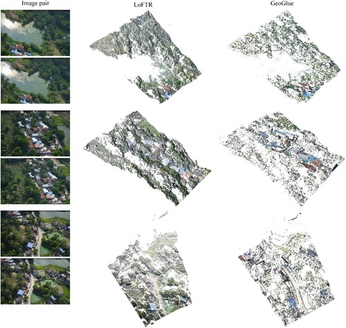
Figures 17–19 provide additional 3D reconstruction results for the fine-grained matching within diverse scenes, and includes comparisons between LoFTR (Sun et al. 2021) and GeoGlue. The results from GeoGlue were observed to feature effective reconstruction for salient geometric elements, e.g. the steps in undulating shapes, serpentine roads, roofs, etc. Since GeoGlue focuses more on geometric objects, however, the reconstruction performance was not satisfactory for natural objects (e.g. trees) and some texture-less planes. Therefore, for GeoGlue, a strategy that spares a certain attention from abundant geometric elements should be considered.

Figure 17. City scenes with large artificial features (e.g. buildings).

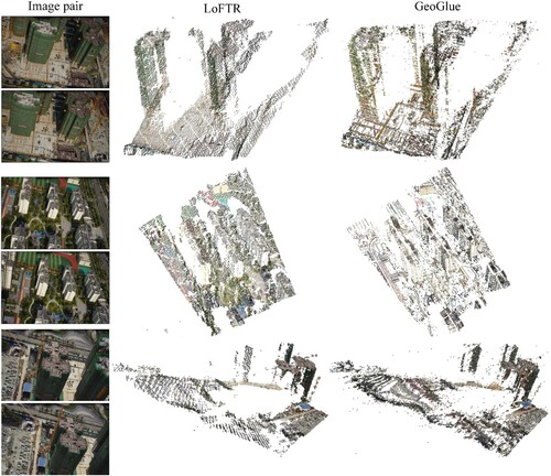
Figure 18. Scenes containing small-sized and delicate artificial features (e.g. sculptures).

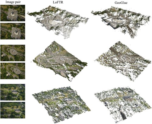
Figure 19. Village scenes.

5. Conclusions and future work

Feature matching is challenging in high-resolution UAV imagery since the visual information is complicated due to the presence of repetitive patterns (e.g. aligned windows on tall buildings), low texture surfaces, shading, and image noise. We propose GeoGlue to overcome these issues. GeoGlue is a novel feature-matching method that contains a self-supervised geometric detector (GD) and a graph attention network (GAT). The method aims to facilitate spatial context awareness during model inference and achieve accurate feature-matching results.

GD is a CNN model within GeoGlue that is trained in a self-supervised manner with synthetic images. Comprehensive experiments confirm the effectiveness and robustness of GD for extracting geometric priors (i.e. keypoints and lines) and providing quality keypoint candidates used in the matching step. In addition, the experiments also demonstrate the feasibility of employing the keypoints obtained from GD for matching based on GNN architecture. The experimental results show the superiority of GeoGlue in terms of matching accuracy and stability under various UAV scenes compared with other learning-based methods. The reliable matching capability of GeoGlue also enables global matching to perform 3D reconstruction through fine-grained matching on high-resolution UAV image pairs.

However, there are still limitations to GeoGlue. Since the GPU memory is finite, it is impractical to use all the keypoints provided by GD to perform feature matching. A strategy that filters out trivial lines must be adopted, which may abandon some quality keypoints that are meaningful for depicting the structural details of small-sized objects. In future studies, more effort will be applied to research on grading keypoints for intelligent keypoint selection in accordance with their importance in structural reconstruction.

Disclosure statement

No potential conflict of interest was reported by the author(s).

Data availability statement

The testing data, which are utilized and support the findings in this paper, are openly available in figshare at URLs: (a) https://figshare.com/ndownloader/files/38095920 and (b) https://figshare.com/ndownloader/files/38945210.

Additional information

Funding

Research presented in this paper was supported by the Strategic Priority Research Program of the Chinese Academy of Sciences [Grant No. XDA19080101], the Director Fund of the International Research Center of Big Data for Sustainable Development Goals [Grant No. CBAS2022DF015], the National Natural Science Foundation of China [Grant No. 41901328 and 41974108], and the National Key Research and Development Program of China [Grant No. 2022YFC3800700].

Appendix A

Data visualization for the pseudo image dataset

An item of training data in the pseudo image dataset is composed of a pseudo image and the corresponding labels (i.e. a line map and a keypoint map). Specific samples referring to the six types of geometry templates (Section 4.1.1) are displayed in Figure 20.

Figure 20. Training data samples of the six types of geometry templates in the pseudo image dataset.

Appendix B. Descriptor visualization

Figure 21. Descriptor visualization for a sample image pair under different component combinations through PCA.

References

- Akinlar, C., and C. Topal. 2011. “EDLines: A Real-Time Line Segment Detector with a False Detection Control.” Pattern Recognition Letters 32 (13): 1633–1642. doi:10.1016/j.patrec.2011.06.001.
- Ballard, D. 1981. “Generalizing the Hough Transform to Detect Arbitrary Shapes.” Pattern Recognition 13: 111–122. doi:10.1016/0031-3203(81)90009-1
- Bay, H., A. Ess, T. Tuytelaars, and L. Van Gool. 2008. “Speeded-Up Robust Features (SURF).” Computer Vision and Image Understanding 110: 346–359. doi:10.1016/j.cviu.2007.09.014.
- Bertasius, G., J. Shi, and L. Torresani. 2015. “DeepEdge: A Multi-Scale Bifurcated Deep Network for Top-Down Contour Detection.” 2015 IEEE Conference on Computer Vision and Pattern Recognition (CVPR), Boston, MA, USA, IEEE, 4380–4389. doi:10.1109/CVPR.2015.7299067.
- Calonder, M., V. Lepetit, C. Strecha, and P. Fua. 2010. “Brief: Binary Robust Independent Elementary Features.” The 11th European Conference on Computer Vision (ECCV), Heraklion, Crete, Greece, Springer-Verlag, 778–792. doi:10.5555/1888089.1888148.
- Canny, J. 1986. “A Computational Approach to Edge Detection.” IEEE Transactions on Pattern Analysis and Machine Intelligence, 679–698. doi:10.1109/TPAMI.1986.4767851.
- Cipolla, R., Y. Gal, and A. Kendall. 2018. “Multi-task Learning Using Uncertainty to Weigh Losses for Scene Geometry and Semantics.” 2018 IEEE/CVF Conference on Computer Vision and Pattern Recognition, Lake City, UT, USA, IEEE, 7482–7491. doi:10.1109/CVPR.2018.00781.
- Cover, T., and P. Hart. 1967. “Nearest Neighbor Pattern Classification.” IEEE Transactions on Information Theory 13: 21–27. doi:10.1109/TIT.1967.1053964.
- Cristina, S.-C., and S. Holban. 2013. “A Comparison of X-Ray Image Segmentation Techniques.” Advances in Electrical and Computer Engineering 13: 85–92. doi:10.4316/AECE.2013.03014.
- de Lima, R., A. A. Cabrera-Ponce, and J. Martinez-Carranza. 2021. “Parallel Hashing-Based Matching for Real-Time Aerial Image Mosaicing.” Journal of Real-Time Image Processing 18: 143–156. doi:10.1007/s11554-020-00959-y.
- de Lima, R., and J. Martinez-Carranza. 2017. “Real-Time Aerial Image Mosaicing Using Hashing-Based Matching.” 2017 Workshop on Research, Education and Development of Unmanned Aerial Systems (RED-UAS), Sweden, IEEE, 144–149. doi:10.1109/RED-UAS.2017.8101658.
- DeTone, D., T. Malisiewicz, and A. Rabinovich. 2018. “SuperPoint: Self-Supervised Interest Point Detection and Description.” 2018 IEEE/CVF Conference on Computer Vision and Pattern Recognition Workshops (CVPRW), Salt Lake City, UT, IEEE, 337–349. doi:10.1109/CVPRW.2018.00060.
- Dusmanu, M., I. Rocco, T. Pajdla, M. Pollefeys, J. Sivic, A. Torii, and T. Sattler. 2019. “D2-Net: A Trainable CNN for Joint Description and Detection of Local Features.” 2019 IEEE/CVF Conference on Computer Vision and Pattern Recognition (CVPR), Long Beach, CA, USA, IEEE, 8084–8093. doi:10.1109/CVPR.2019.00828.
- Grompone von Gioi, R., J. Jakubowicz, J. Morel, and G. Randall. 2010. “LSD: A Fast Line Segment Detector with a False Detection Control.” IEEE Transactions on Pattern Analysis and Machine Intelligence 32 (4): 722–732. doi:10.1109/TPAMI.2008.300.
- Han, X., T. Leung, Y. Jia, R. Sukthankar, and A. C. Berg. 2015. “MatchNet: Unifying Feature and Metric Learning for Patch-Based Matching.” 2015 IEEE Conference on Computer Vision and Pattern Recognition (CVPR), Boston, MA, USA, IEEE, 3279–3286. doi:10.1109/CVPR.2015.7298948.
- Hartley, R. I. 1995. “In Defence of the 8-Point Algorithm.” IEEE International Conference on Computer Vision (ICCV), Cambridge, MA, USA, IEEE, 1064–1070. doi:10.1109/ICCV.1995.466816.
- He, M., Q. Guo, A. Li, J. Chen, B. Chen, and X. Feng. 2018. “Automatic Fast Feature-Level Image Registration for High-Resolution Remote Sensing Images.” Journal of Remote Sensing 22 (2): 277–292. doi:10.11834/jrs.20186420.
- He, J., S. Zhang, M. Yang, Y. Shan, and T. Huang. 2022. “BDCN: Bi-Directional Cascade Network for Perceptual Edge Detection.” IEEE Transactions on Pattern Analysis and Machine Intelligence 44: 100–113. doi:10.1109/TPAMI.2020.3007074.
- Huang, P.-H., K. Matzen, J. Kopf, N. Ahuja, and J.-B Huang. 2018a. “DeepMVS: Learning Multi-View Stereopsis.” 2018 IEEE/CVF Conference on Computer Vision and Pattern Recognition (CVPR), Salt Lake City, UT, USA, IEEE, 2821–2830. doi:10.1109/CVPR.2018.00298.
- Huang, K., Y. Wang, Z. Zhou, T. Ding, S. Gao, and Y. Ma. 2018b. “Learning to Parse Wireframes in Images of Man-Made Environments.” 2018 IEEE/CVF Conference on Computer Vision and Pattern Recognition (CVPR), Salt Lake City, UT, USA, IEEE, 626–635. doi:10.1109/CVPR.2018.00072.
- Kittler, J. 1983. “On the Accuracy of the Sobel Edge Detector.” Image and Vision Computing 1 (1): 37–42. doi:10.1016/0262-8856(83)90006-9
- Knapitsch, A., J. Park, Q. Y. Zhou, and V. Koltun. 2017. “Tanks and Temples: Benchmarking Large-Scale Scene Reconstruction.” ACM Transactions on Graphics 36 (4): 1. doi:10.1145/3072959.3073599
- Lee, J. H., S. Lee, G. Zhang, J. Lim, W. K. Chung, and I. H. Suh. 2014. “Outdoor Place Recognition in Urban Environments Using Straight Lines.” 2014 IEEE International Conference on Robotics and Automation (ICRA), Hong Kong, China, IEEE, 5550–5557. doi:10.1109/ICRA.2014.6907675.
- Leutenegger, S., M. Chli, and R. Y. Siegwart. 2011. “Brisk: Binary Robust Invariant Scalable Keypoints.” 2011 International Conference on Computer Vision (ICCV), Barcelona, Spain, IEEE, 2548–2555. doi:10.1109/ICCV.2011.6126542.
- Li, J., T. Yang, J. Yu, Z. Lu, P. Lu, X. Jia, and W. Chen. 2014. “Fast Aerial Video Stitching.” International Journal of Advanced Robotic Systems 11 (10): 167. doi:10.5772/59029.
- Li, H., H. Yu, J. Wang, W. Yang, L. Yu, and S. Scherer. 2021. “ULSD: Unified Line Segment Detection Across Pinhole, Fisheye, and Spherical Cameras.” ISPRS Journal of Photogrammetry and Remote Sensing 178: 187–202. doi:10.1016/j.isprsjprs.2021.06.004.
- Lowe, D. G. 2004. “Distinctive Image Features from Scale-Invariant Keypoints.” International Journal of Computer Vision 60 (2): 91–110. doi:10.1023/B:VISI.0000029664.99615.94
- Lu, X., J. Yao, K. Li, and L. Li. 2015. “CannyLines: A Parameter-Free Line Segment Detector.” 2015 IEEE International Conference on Image Processing (ICIP), Quebec City, QC, Canada, IEEE, 507–511. doi:10.1109/ICIP.2015.7350850.
- Luo, Z., T. Shen, L. Zhou, J. Zhang, Y. Yao, S. Li, T. Fang, and L. Quan. 2019. “ContextDesc: Local Descriptor Augmentation With Cross-Modality Context.” 2019 IEEE/CVF Conference on Computer Vision and Pattern Recognition (CVPR), Long Beach, CA, USA, IEEE, 2522–2531. doi:10.1109/CVPR.2019.00263.
- Melekhov, I., A. Tiulpin, T. Sattler, M. Pollefeys, E. Rahtu, and J. Kannala. 2019. “DGC-Net: Dense Geometric Correspondence Network.” 2019 IEEE Winter Conference on Applications of Computer Vision (WACV), Waikoloa, HI, USA, IEEE, 1034–1042. doi:10.1109/WACV.2019.00115.
- Mur-Artal, R., and J. D. Tardós. 2017. “ORB-SLAM2: An Open-Source SLAM System for Monocular, Stereo, and RGB-D Cameras.” IEEE Transactions on Robotics 33 (5): 1255–1262. doi:10.1109/TRO.2017.2705103.
- Newell, A., K. Yang, and J. Deng. 2016. “Stacked Hourglass Networks for Human Pose Estimation.” European Conference on Computer Vision (ECCV), Springer, 483–499. doi:10.1007/978-3-319-46484-8_29.
- Ono, Y., E. Trulls, P. Fua, and K. M. Yi. 2018. “LF-Net: Learning Local Features from Images.” 2018 Neural Information Processing Systems (NeurIPS), NY, USA, Curran Associates Inc., 6237–6247. doi:10.5555/3327345.3327521.
- Pautrat, R., J.-T. Lin, V. Larsson, M. R. Oswald, and M. Pollefeys. 2021. “SOLD2: Self-Supervised Occlusion-Aware Line Description and Detection.” 2021 IEEE/CVF Conference on Computer Vision and Pattern Recognition (CVPR), Nashville, TN, USA, IEEE, 11363–11373. doi:10.1109/CVPR46437.2021.01121.
- Prewitt, J. M. S. 1970. “Object Enhancement and Extraction.” Picture Processing and Psychopictorics, 75–149.
- Pu, M., Y. Huang, Y. Liu, Q. Guan, and H. Ling. 2022. “EDTER: Edge Detection with Transformer.” 2022 IEEE/CVF Conference on Computer Vision and Pattern Recognition (CVPR), New Orleans, LA, USA, IEEE, 1392–1402. doi:10.1109/CVPR52688.2022.00146.
- Revaud, J., P. Weinzaepfel, C. R. de Souza, N. Pion, G. Csurka, Y. Cabon, and M. Humenberger. 2019. “R2D2: Repeatable and Reliable Detector and Descriptor.” 2019 Neural Information Processing Systems (NeurIPS), Vancouver, British Columbia, Canada, Curran Associates Inc 12414–12424. doi:10.5555/3454287.3455400.
- Rublee, E., V. Rabaud, K. Konolige, and G. Bradski. 2011. “ORB an Efficient Alternative to SIFT or SURF.” 2011 International Conference on Computer Vision (ICCV), Barcelona, SPAIN, IEEE, 2564–2571. doi:10.1109/ICCV.2011.6126544.
- Sarlin, P.-E., D. DeTone, T. Malisiewicz, and A. Rabinovich. 2020. “SuperGlue: Learning Feature Matching With Graph Neural Networks.” 2020 IEEE/CVF Conference on Computer Vision and Pattern Recognition (CVPR), Seattle, WA, USA, IEEE, 4937–4946. doi:10.1109/CVPR42600.2020.00499.
- Savinov, N., A. Seki, L. Ladický, T. Sattler, and M. Pollefeys. 2017. “Quad-Networks: Unsupervised Learning to Rank for Interest Point Detection.” 2017 IEEE Conference on Computer Vision and Pattern Recognition (CVPR), Honolulu, HI, USA, IEEE, 3929–3937. doi:10.1109/CVPR.2017.418.
- Schönberger, J. L., and J.-M. Frahm. 2016. “Structure-from-Motion Revisited.” 2016 IEEE Conference on Computer Vision and Pattern Recognition (CVPR), Las Vegas, NV, USA, IEEE, 4104–4113. doi:10.1109/CVPR.2016.445.
- Schöps, T., J. L. Schönberger, S. Galliani, T. Sattler, K. Schindler, M. Pollefeys, and A. Geiger. 2017. “A Multi-View Stereo Benchmark with High-Resolution Images and Multi-Camera Videos.” 2017 IEEE/CVF Conference on Computer Vision and Pattern Recognition, Honolulu, HI, USA, IEEE, 2538–2547. doi:10.1109/CVPR.2017.272.
- Shi, W., J. Caballero, F. Huszár, J. Totz, A. P. Aitken, R. Bishop, D. Rueckert, and Z. Wang. 2016. “Real-Time Single Image and Video Super-Resolution Using an Efficient Sub-Pixel Convolutional Neural Network.” 2016 IEEE Conference on Computer Vision and Pattern Recognition (CVPR), Las Vegas, NV, USA, IEEE, 1874–1883. doi:10.1109/CVPR.2016.207.
- Simo-Serra, E., E. Trulls, L. Ferraz, I. Kokkinos, P. Fua, and F. Moreno-Noguer. 2015. “Discriminative Learning of Deep Convolutional Feature Point Descriptors.” 2015 IEEE International Conference on Computer Vision (ICCV), Santiago, Chile, IEEE, 118–126. doi:10.1109/ICCV.2015.22.
- Sinkhorn, R., and P. Knopp. 1967. “Concerning Nonnegative Matrices and Doubly Stochastic Matrices.” Pacific Journal of Mathematics 21 (2): 343–348. doi:10.2140/pjm.1967.21.343
- Sun, J., Z. Shen, Y. Wang, H. Bao, and X. Zhou. 2021. “LoFTR: Detector-Free Local Feature Matching with Transformers.” 2021 IEEE/CVF Conference on Computer Vision and Pattern Recognition (CVPR), Nashville, TN, USA, IEEE, 8918–8927. doi:10.1109/CVPR46437.2021.00881.
- Vaswani, A., N. Shazeer, N. Parmar, J. Uszkoreit, L. Jones, A. N. Gomez, L. Kaiser, and I. Polosukhin. 2017. “Attention is all you Need.” 2017 International Conference on Neural Information Processing Systems (NeurIPS). Red Hook, NY, USA, Curran Associates Inc., 6000–6010. doi:10.5555/3295222.3295349.
- Wang, G., Z. Zhai, B. Xu, and Y. Cheng. 2017. “A Parallel Method for Aerial Image Stitching Using orb Feature Points.” 2017 IEEE/ACIS 16th International Conference on Computer and Information Science (ICIS), Wuhan, China, IEEE, 769–773. doi:10.1109/ICIS.2017.7960096.
- Wei, X., Y. Zhang, Z. Li, Y. Fu, and X. Xue. 2020. “DeepSFM: Structure from Motion via Deep Bundle Adjustment.” 2020 European Conference on Computer Vision (ECCV), Glasgow, UK, Springer, 230–247. doi:10.1007/978-3-030-58452-8_14.
- Xue, N., S. Bai, F. Wang, G. Xia, T. Wu, and L. Zhang. 2019. “Learning Attraction Field Representation for Robust Line Segment Detection.” 2019 IEEE/CVF Conference on Computer Vision and Pattern Recognition (CVPR), Long Beach, CA, USA, IEEE, 1595–1603. doi:10.1109/CVPR.2019.00169.
- Xue, N., T. Wu, S. Bai, F. Wang, G. S. Xia, L. Zhang, and P. H. S. Torr. 2020. “Holistically-Attracted Wireframe Parsing.” 2020 IEEE/CVF Conference on Computer Vision and Pattern Recognition (CVPR), Seattle, WA, USA, IEEE, 2785–2794. doi:10.1109/CVPR42600.2020.00286.
- Yi, K. M., E. Trulls, V. Lepetit, and P. Fua. 2016. “Lecture Notes in Computer Science.” 2016 European Conference on Computer Vision (ECCV), Springer, 467–483. doi:10.1007/978-3-319-46466-4_28.
- Yu, Z., C. Feng, M.-Y. Liu, and S. Ramalingam. 2017. “CASENet: Deep Category-Aware Semantic Edge Detection.” 2017 IEEE Conference on Computer Vision and Pattern Recognition (CVPR), Honolulu, HI, USA, IEEE, 1761–1770. doi:10.1109/CVPR.2017.191.
- Zhang, Z. 1998. “Determining the Epipolar Geometry and its Uncertainty: A Review.” International Journal of Computer Vision 27 (2): 161–195. doi:10.1023/A:1007941100561
- Zhou, Y., H. Qi, and Y. Ma. 2019. “End-to-End Wireframe Parsing.” 2019 IEEE/CVF International Conference on Computer Vision (ICCV), Seoul, Korea (South), IEEE, 962–971. doi:10.1109/ICCV.2019.00105