Integration of Landsat time-series vegetation indices improves consistency of change detection

ABSTRACT

Vegetation indices (VIs) were used to detect when and where vegetation changes occurred. However, different VIs have different or even diametrically opposite results, which obstructed the in-depth understanding of vegetation change. Therefore, this study examined the spatial and temporal consistency of five VIs (EVI; NBR; NDMI; NDVI; and NIRv) in detecting abrupt and gradual vegetation changes, and provided an ensemble algorithm which integrated the change detection results of the five indices to reduce the uncertainty of change detection using a single index. The spatial consistency of the five indices in abrupt change detection accounted for 50.6% of the study area, but the temporal consistency was low (21.6%). Wetness indices (NBR, NDMI) were more sensitive to negative abrupt changes, greenness indices (EVI, NDVI, NIRv) were more sensitive to positive abrupt changes; and both types of indices were similar in detecting gradual and total changes. The overall accuracy of the ensemble method was 81.60% and higher than that of any single index in abrupt change detection. This study provides a comprehensive evaluation of the spatial and temporal inconsistencies of change detection in model-fitting errors and various types of vegetation changes. The proposed ensemble method can support robust change-detection.

KEYWORDS:

• Breaks for Additive Season and Trend
• ensemble algorithm
• consistence of vegetation change
• vegetation index

1. Introduction

Vegetation controls the exchange of carbon, water, momentum and energy between the land and the atmosphere, and provides food, fibre, fuel and other ecosystem services (Haberl et al. 2007; Bonan, Pollard, and Thompson 1992). Vegetation changes can be grouped into three categories: (1) seasonal, caused by vegetation phenology; (2) gradual, caused by climate change, vegetation growth, and degradation in longer-term processes; and (3) abrupt, caused by natural and human disturbance such as wildfire, typhoon, earthquake, urbanization, deforestation, and afforestation (Verbesselt et al. 2010; Fang et al. 2018; Zhu et al. 2016; Li et al. 2021). Abrupt and gradual change refer to trend component beyond the seasonal variation (De Jong et al. 2012). They have critical impacts on long-term vegetation composition and structure, and stability. It is important to systematically collect information on abrupt and gradual changes as indicators of vegetation response to climate change and human activities.

Time series of vegetation indices/reflectance from remotely sensed data provide a unique means to investigate these vegetation changes from local to global at a high frequency of observations (Li et al. 2021). Green vegetation absorbs visible bands and reflects the near infrared (NIR) band, and water in leaves absorbs the shortwave infrared (SWIR) band (Kulawardhana 2011). Spectral response to different plant characteristics provides the basis for monitoring vegetation change using bands or vegetation indices. Spectral indices have an advantage over single bands by amplifying desired effects (e.g. changes in vegetation condition) and reducing unwanted features (e.g. atmospheric and topographic noise) (Matsushita et al. 2007). Vegetation indices (VIs), such as normalized difference vegetation index (NDVI) (Verbesselt et al. 2010; DeVries et al. 2015), enhanced vegetation index (EVI) (Grogan et al. 2016), normalized difference moisture index (NDMI) (Murillo-Sandoval et al. 2018; Schultz et al. 2018), and normalized burn ratio (NBR) (Esteban et al. 2021), are the most common indicators detecting vegetation changes. These vegetation indices are divided into the greenness index combining red and NIR bands, and wetness index combining SWIR and NIR bands. NDVI and EVI are greenness indices and highly related to the amount of chlorophyll, vegetation leaf area, and photosynthetic capacity (Huete et al. 2002; Tucker 1979). Compare to NDVI, EVI is generally more robust to atmospheric and soil background influences, and saturates less at high biomass levels (Huete et al. 2002). NBR and NDMI are wetness indices and sensitive to forest structure, moisture, shadowing, and vegetation density (Schroeder et al. 2011). NDVI performs less effectively than NBR for accurate detection of subtler disturbance signals in western Oregon (Kennedy, Yang, and Cohen 2010). The signals of the various indices associated with vegetation change differ significantly from each other, especially for subtle changes (Kennedy, Yang, and Cohen 2010; Schultz et al. 2016; Hislop et al. 2019). The VIs-based change-detection results can vary between indices, sensors, quality-control measures, compositing algorithms, and atmospheric and sun-target-sensor geometry corrections (Zeng et al. 2022). These variations make it difficult to draw robust conclusions about ecosystem change and highlight the need for consistent vegetation index application and verification (Bueno et al. 2020; Zeng et al. 2022).

Previous researches using linear regression models (e.g. Mann-Kendall test and Theil-Sen estimator) over the entire period showed that vegetation areas have experienced inconsistent change trends in greenness, coverage, and productivity (Berner and Goetz 2022; Ding et al. 2020). However, overall linear change trend analysis usually ignores the impact of abrupt change on the long-term vegetation change characteristics (He et al. 2021). Zhu and Woodcock (2014) and De Jong et al. (2012) found that considering abrupt change is a critical premise and foundation to accurately describe the vegetation change processes. Bueno et al. (2020) find a low rate of spatial agreement among seven index-based disturbance maps. There are very few studies on the differences among vegetation indices in characterizing both abrupt and gradual vegetation changes.

The various vegetation indices perform well in terms of disturbance detection, but there is a large inconsistency among detection results of various indices (Bueno et al. 2020). Vegetation change detected by several spectral indices simultaneously may separate forest disturbance signals from noise compared to a single spectral index (Shimizu et al. 2019). Combining several vegetation indices or change-detection results may resolve some of difference and complement their merits, and has become an important means to increase the robustness of vegetation change monitoring. The ensemble methods for change detection applications have used different approaches to deciding change, including voting (e.g. majority), rule-based decisions (Saxena et al. 2017), and stacking using the Random Forest method (Schultz et al. 2016; Cohen et al. 2018). Stacking using a Random Forest model has become a popular method due to its high accuracy. However, the demand for reliable historical samples limits its application in subtropical regions. Training and validation data are very scarce due to complex drivers of vegetation change and frequent cloud cover in the reference images (e.g. Landsat).

In this study, we investigated the spatial and temporal differences of the change-detection results from different vegetation indices and integrated the results. Specifically, five vegetation indices from Landsat and the BFAST (Breaks For Additive Season and Trend) method were used to calculate the abrupt, gradual, and total vegetation change in China’s Wuyishan National Park and its peripheral areas between 1986 and 2020. The objectives of this research were to examine the differences of five vegetation indices in model fitting during BFAST change detection, and the spatial and temporal inconsistencies of the vegetation change processes (including abrupt, gradual, and total changes), and to improve change-detection accuracy by integrating the results of different vegetation indices.

2. Study area

The study area is located in Wuyishan National Park and its peripheral areas (Figure 1). Wuyishan National Park, which is one of the first established national parks in China, integrates five different types of protected areas and has the most complete, typical, and largest primeval forest ecosystem in the subtropical region at the same latitude on Earth. The vegetation inside the park is strictly protected, and any human disturbance was forbidden. However, natural disasters (e.g. extreme drought in 2003, heavy snowfall in 2007) have significantly influenced the vegetation dynamics. In addition, the contradiction between economic development needs and vegetation protection still exists in the park, leading to frequent reclamation and interplanting of tea on the forested lands. The peripheral areas lack relevant policy support and abrupt changes were partly driven by harvest, urbanization, and land use with large area of pure coniferous plantation. The inside and outside of the park represent different disturbance regimes, allowing comparison of spectral, temporal and spatial disturbance patterns on a gradient from a natural system to a human and natural coupling system.

Figure 1. Location of the study area (a, and b) and land-cover types in the study area (c) (Fan et al. 2022).

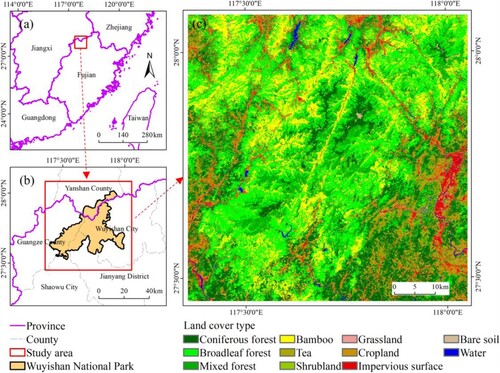
The terrain of the study area is complex, with an altitude range of 30–2154 m and a typical subtropical monsoon climate with four distinct seasons. The annual average temperature is 18.3 ℃, the average annual precipitation is 1926.9 mm, and the annual average relative humidity is 78% (Lin et al. 2020). The vegetation cover types have obvious vertical zone change, including mainly broadleaf forest (32.53%), coniferous forest (18.95%), bamboo (16.63%), tea (11.76%), and mixed coniferous and broadleaf forest (10.47%) (Figure 1c).

3. Methods

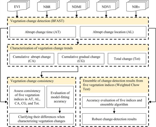
The methodology flowchart is shown in Figure 2, and includes (1) a comprehensive evaluation of the spatial and temporal consistencies of change detection in both model-fitting errors and various types of vegetation changes, and (2) a robust change-detection result by integrating different vegetation indices.

Figure 2. The methodology flowchart for the current research.

3.1. Data preparation

3.1.1. Landsat data acquisition and preprocessing

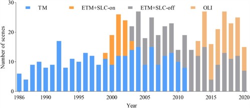
All available Landsat 5, 7, and 8 images (Worldwide Reference System [WRS] Path 120 and Row 41) with more than 20% clear observations (i.e. pixels with no clouds, cloud shadows, or snow) between 1986 and 2020 were acquired from the United States Geological Survey (USGS) through bulk ordering (https://espa.cr.usgs.gov/) (Figure 3). A total of 583 images (TM: 276, ETM + SLC-on: 41, ETM + SLC-off: 178, OLI: 88) were collected from Landsat Collection 1 Surface Reflectance Level-2 products, which had been preprocessed with geo-referencing, automatic atmospheric correction, and clouds and shadows detection by USGS. Only terrain corrected data (L1T) were used. The Landsat 5/7 surface reflectance data were atmospherically corrected using the Landsat Ecosystem Disturbance Adaptive Processing System (LEDAPS) algorithm (Masek et al. 2006), and the Landsat 8 surface reflectance were generated using the Land Surface Reflectance Code (LaSRC) (Vermote et al. 2016) algorithm. Clouds, cloud shadows, and stripes were masked in each image, and all clear observations were retained based on the pixel quality assurance (QA) data created from a CFMask algorithm (Z. Zhu and Woodcock 2012).

Figure 3. The number of Landsat scenes from 1986 to 2020 used in this study.

3.1.2. Vegetation indices

NBR, NDMI, NDVI and EVI are commonly used indices to track vegetation change. NIRv is the latest proposed vegetation index and has a more direct physical interpretation than traditional vegetation indices (Badgley, Field, and Berry 2017), which has not been used in the field of vegetation change detection. These selected spectral indices are readily comparable since they depict vegetation greenness and moisture content, which can be used as indications of vegetation health (Bullock, Woodcock, and Holden 2020). The higher values in these indices indicate better condition of the vegetation. The values of these indices are between −1 and 1.

Four commonly used vegetation index products – EVI, NBR, NDMI, and NDVI – were downloaded from USGS Earth Resources Observation and Science (EROS) Center Science Processing Architecture (ESPA) (https://espa.cr.usgs.gov/), and the near-infrared reflectance of vegetation (NIRv) time series were calculated from the acquired Landsat surface reflectance products. Details about the five vegetation indices are listed in Table 1.

Table 1. Vegetation indices used in this study.

VI	Equation	Remarks	Reference
EVI	${\displaystyle \frac{2.5(p_{NIR}-p_R)}{p_{NIR}+6p_R-7.5p_B+1}}$	Sensitive to plant canopy and growing conditions	Huete et al. (2002)
NBR	${\displaystyle \frac{p_{NIR}-p_{SWIR2}}{p_{NIR}+p_{SWIR2}}}$	Sensitive to disturbance and fire	García and Caselles (1991)
NDMI	${\displaystyle \frac{p_{NIR}-p_{SWIR1}}{p_{NIR}+p_{SWIR1}}}$	Sensitive to canopy moisture content	Vogelmann and Rock (1988)
NDVI	${\displaystyle \frac{p_{NIR}-p_R}{p_{NIR}+p_R}}$	Sensitive to photosynthetic activities	Rouse et al. (1976)
NIRv	${\displaystyle \frac{p_{NIR}-p_R}{p_{NIR}+p_R}\ast p_{NIR}}$	Sensitive to canopy variation	Badgley, Field, and Berry (2017)

Notes: VI, vegetation index; $p_{NIR}$,$p_R$, $p_B$, $p_{SWIR1}$, and $p_{SWIR2}$ are the near infrared, red, blue, first shortwave infrared, and second shortwave infrared bands, respectively.

3.2. Vegetation change detection and characterization

3.2.1. Detection of abrupt vegetation change

The BFAST (Breaks for Additive Season and Trend) method allows the detection of multiple breakpoints while explicitly considering seasonal variations, and identifies both gradual and abrupt changes in time series (Verbesselt et al. 2010). This algorithm has been successfully applied in several ecosystems (Fang et al. 2018). Besides, it is more efficient than other change detection algorithms because it does not require a threshold setting and is ‘data-driven’ (DeVries et al. 2015), and is more suitable for noisy datasets (Awty-Carroll et al. 2019). Change detection was performed for each pixel using the BFAST algorithm (Verbesselt et al. 2010; Verbesselt, Hyndman, Zeileis, et al. 2010). First, the time-series data were tested for the presence of one or more breakpoints based on the ordinary least squares residuals-based moving sum (OLS-MOSUM). The breakpoint equals to abrupt change in the time series vegetation index, which means a large magnitude of vegetation change and/or changes in trends accompanying a sudden disturbance event (Li et al. 2021). If the test showed no abrupt change in the time series of a pixel, a harmonic model of Equation. (1) (Verbesselt, Hyndman, Zeileis, et al. 2010) was built for the whole time series. Otherwise, the following three steps were used for the time series: (1) calculate the corresponding minimum residual sum of squares (RSS) for different numbers of breakpoints; (2) determine the optimal segmentation scheme of the model based on the minimization Bayesian Information Criterion (BIC); (3) record the number of breakpoints determined by BIC and the time of the breakpoints determined by the minimum residual sum of squares (RSS). According to the number and time of breakpoints, the harmonic model in our study was built for each segment, and coefficients of each segment were output for each pixel. (1) $\hat{p}(i,t{)}_{VI}={\beta }_i+a_i\cos \left({\displaystyle \frac{2\pi }{T}t}\right)+b_i\sin \left({\displaystyle \frac{2\pi }{T}t}\right)+c_{i}t$(1) where i is the i-th segment, ${\tau }_k^{\ast }$ is the k-th breakpoint, t is the observation time, $\hat{p}$ is the fitted vegetation index (VI) value, $\beta$ is the intercept, a and b are the seasonal and phased harmonic components of different frequencies characterizing the seasonal variation of vegetation; c is the trend of VI; and T is 365 days per year.

The BFAST method uses the parameters of the minimum segment size (h) and maximum abrupt change times to control the change-detection process (Li et al. 2021). According to Dutrieux et al. (2016) and Li et al. (2018), the minimum segment size was set to 0.15 to ensure there were enough observations to fit the harmonic model. Considering the relatively low disturbance in the study area, the maximum time of vegetation changes was set to 6, indicating a maximum of 6 possible breakpoints throughout the study period.

3.2.2. Characterization of vegetation change

We focused on abrupt and gradual changes in this study considering that these two changes over times served as good indicators of vegetation response to climate change and human activities (Zhu et al. 2016). Gradual and abrupt change vary by severity and length of the time of impact on vegetation. Gradual change indicates the lower severity change occurring over long periods of time (5 + years), and abrupt change associates with high-severity and short-duration vegetation change accompanying a sudden disturbance event (De Jong et al. 2012; Zhu et al. 2016; Li et al. 2021). Positive and negative vegetation changes were referred to as greening and browning, respectively (De Jong et al. 2012).

Equation (2(2) $V{I}_{end,i}=a_i+t_{end,i}\times c_i$(2) ) was used to calculate the overall vegetation index at the beginning and end times of each segment for each pixel. Equations (3), (4), and (5) defined the cumulative abrupt change ($C{A}_{VI}$), cumulative gradual change ($C{G}_{VI}$), and total change ($To{t}_{VI}$), respectively. $C{A}_{VI}$ is the sum of abrupt change and indicates the net effect of rapid disturbances on vegetation cover between 1986 and 2020. $C{G}_{VI}$ is the sum of gradual change and indicates the changing trend of the vegetation index between 1986 and 2020. $To{t}_{VI}$ is the sum of abrupt change and gradual change and reflects the total improvement or degradation of vegetation between 1986 and 2020 (Li et al. 2018; Zhu et al. 2016). $C{G}_{VI}$ is equal to $To{t}_{VI}$ for the pixels that had no abrupt changes. (2) $V{I}_{end,i}=a_i+t_{end,i}\times c_i$(2) (3) $C{A}_{VI}=\sum _{i=1}^{K-1}(V{I}_{start,i+1}-V{I}_{end,i})$(3) (4) $C{G}_{VI}=\sum _{i=1}^K(V{I}_{end,i}-V{I}_{start,i})$(4) (5) $To{t}_{VI}=C{G}_{VI}+C{A}_{VI}$(5) where $a_i$ and $c_i$ are the intercept and slope of the interannual variation of the i-th segment; $t_{start,i}$ and $t_{end,i}$ are the start and end times of the i-th segment (Julian days); $V{I}_{start,i}$ and $V{I}_{end,i}$ are the vegetation indices at the start and end time of the segment; K is segment number divided by disturbances for each pixel.

3.3. Vegetation change consistencies of five vegetation indices

3.3.1. Evaluation of model-fitting accuracy

Vegetation indices might have different responses and characteristics to the same vegetation change process, and lead to different change-detection results (Bueno et al. 2020). We proposed a consistent framework for evaluating vegetation changes based on our chosen vegetation indices. Normalized root mean square error (NRMSE) (Mayer and Butler 1993) and Willmott's index of agreement (WIA) (Willmott 1981) were used to analyze the model-fitting accuracies of the five vegetation indices based on the change-detection mechanism of BFAST. NRMSE has the advantage of comparing datasets or models at different scales. Its value is between 0 and 1, where 0 indicates good model accuracy, values smaller than 0.2 represent acceptable model accuracy, and values higher than 0.2 indicate unacceptable model accuracy (Zhu et al. 2019). WIA is a standardized index used to evaluate the model’s prediction error and systematic error (Xin et al. 2020). WIA ranges from 0 to 1, where 1 indicates a robust positive correlation and 0 indicates no relationship between actual and predicted values (Abdullah et al. 2019). The formulas are as follows: (6) $\mathrm{RMSE}=\sqrt{{\displaystyle \frac{\sum {({\hat{y}}_i-y_i)}^2}{n}}}$(6) (7) $\mathrm{NRMSE}={\displaystyle \frac{RMSE}{Q_3-Q_1}}$(7) (8) $\mathrm{WIA}=1-{\displaystyle \frac{{\sum }_{i=1}^n{(y_i-{\hat{y}}_i)}^2}{{\sum }_{i=1}^n{(|{\hat{y}}_i-\overline{y}|+|y_i-\overline{y}|)}^2}}$(8) where $y_i$ is the observed value at time i; ${\hat{y}}_i$ is the predicted value at time i; $\overline{y}$ is the average observed value; n is the number of observations; $Q_1$ is the lower quartile, and $Q_3$ is the upper quartile.

3.3.2. Vegetation change consistency evaluation scheme

An evaluation scheme was constructed to assess the spatial and temporal consistencies of the abrupt change location consistency (ALC) and abrupt change time consistency (ATC), and the vegetation change trend consistency (cumulative abrupt change consistency, CAC; cumulative gradual change consistency, CGC; total change consistency, TotC). All consistencies except ATC were obtained by summing five binary maps (Figure 4a). For ALC, ‘0’ and ‘1’ in the binary map represent no abrupt change and abrupt change, respectively. The agreement counts range from ‘0’ (no abrupt changes were detected by any of the five indices for the pixel) to ‘5’ (abrupt changes were detected by all five indices for the pixel). ATC was obtained by finding the frequency of the modes for all years (ranging from 0 to 30) detected by five indices (Figure 4b). The agreement counts ranged from ‘0’ (none of the five indices detected abrupt change in that year) to ‘5’ (all five indices detected abrupt changes in the same year).

Figure 4. Schematic diagrams of consistency analysis method for five vegetation indices. (a) ALC, CAC, CGC, and TotC were obtained by summing five binary maps respectively. (b) ATC was obtained by considering whether the abrupt change was detected in the same year. Note: NIRv-6 is the year of the sixth breakpoint detected by NIRv, NDVI-1 is the year of the first breakpoint detected by NDVI, and so on.

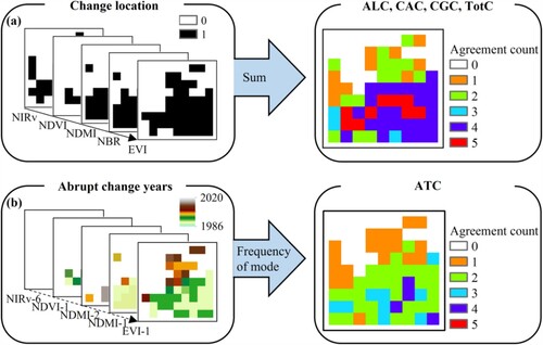
For CAC, CGC, and TotC, ‘0’ and ‘1’ in the binary map represent non-negative vegetation change trends (CA, CG, and Tot are greater than or equal to 0) and negative vegetation change trends (CA, CG, and Tot are lower than 0), respectively. The agreement counts ranged from ‘0’ (vegetation changes of the five indices were all non-negative for a pixel) to ‘5’ (vegetation changes of the five indices were all negative for a pixel). There are 32 different combinations ($C_5^0+C_5^1+C_5^2+C_5^3+C_5^4+C_5^5$) for the five vegetation indices. We further evaluated the contribution of each index to the divergence of abrupt change detection by analyzing which combination contributed the most to ‘1’ and ‘2’.

3.4. Ensemble of change-detection results from five vegetation indices

The breakpoints detected by BFAST are statistically significant in the entire time series, but spurious breakpoints might be detected when the time-series data contain multiple outliers, such as noises from the unmasked clouds. In addition, multiple breakpoints might be detected by different vegetation indices for a very short period. It is reasonable and necessary to evaluate which breakpoints need to be retained and which should be deleted. We proposed an ensemble algorithm to integrate the change-detection results from five vegetation indices. First, Chow Test was used to test the significance of breakpoints (at least two indices detected this breakpoint) in each vegetation index time series, which is expressed by the F-statistic (Equation (9(9) $F(C)={\displaystyle \frac{(SS{R}_C-(SS{R}_1+SS{R}_2))/k}{(SS{R}_1+SS{R}_2)/(n_1+n_2-2k)}}$(9) )). Chow Test was used in economics to assess structural instability in a model when a potential breakpoint is known (Zeileis et al. 2002). Second, the change-detection results of different vegetation indices were integrated through weight rules (Equation (10(10) $\mathrm{F}(\hat{C})={\displaystyle \frac{{\sum }_{q=1}^N{w}_{q}F{(C)}_q}{{\sum }_{q=1}^N{w}_q}}$(10) )). 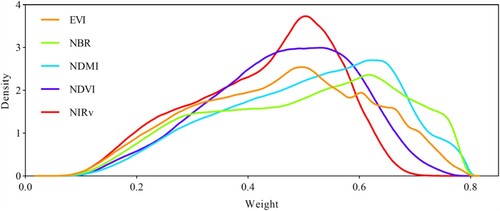The weight was calculated according to the correlations among different vegetation indices (Equation (11(11) $w_q=1-{\displaystyle \frac{{\sum }_{p=1}^N{r}_{pq}}{N}}$(11) )). The corresponding weight will be small if the correlation coefficient among vegetation indices is large. The weights of the five vegetation indices are shown in Figure 5. Finally, if the mean F-statistic is below the critical value, the two models are combined; otherwise, the breakpoint is retained. The breakpoint with the largest F value is considered the most important breakpoint in the entire time series. (9) $F(C)={\displaystyle \frac{(SS{R}_C-(SS{R}_1+SS{R}_2))/k}{(SS{R}_1+SS{R}_2)/(n_1+n_2-2k)}}$(9) (10) $\mathrm{F}(\hat{C})={\displaystyle \frac{{\sum }_{q=1}^N{w}_{q}F{(C)}_q}{{\sum }_{q=1}^N{w}_q}}$(10) (11) $w_q=1-{\displaystyle \frac{{\sum }_{p=1}^N{r}_{pq}}{N}}$(11) where $SS{R}_C$ is the sum of squared residuals from the combined data, $SS{R}_1$ and $SS{R}_2$ are the sums of squared residuals from each group before and after the breakpoint, n is the number of observations for combined data, k is the number of parameters, $w_q$ is the weight coefficient of $V{I}_q$, N is the number of vegetation indices, $r_{pq}$ is the correlation coefficient ($r^2$) between $V{I}_p$ and $V{I}_q$, $F(C{)}_q$ is the test statistic of $V{I}_q$, and F($\hat{C}$) is the mean test statistic across indices.

Figure 5. The weight kernel densities of the five vegetation indices in the ensemble method.

3.5. Accuracy assessment

The performances of five indices in detecting abrupt vegetation change were evaluated at both temporal and spatial scales. A stratified random sampling method was adopted (Schultz et al. 2016), and 100 reference points were randomly selected in each of the five abrupt change maps, with 50 samples in abrupt change areas and 50 samples in non-abrupt change areas. A total of 500 (5 × 100) reference samples were collected. The primary and optimal source for reference data is the Landsat images themselves (Cohen, Yang, and Kennedy 2010; Z. Zhu and Woodcock 2014; Wu et al. 2020). Meanwhile, high spatial resolution images from Google Earth help manual interpretation of the land cover classes and change. We manually interpreted each sample and its adjacent eight pixels using Google high-resolution images and Landsat time-series images for determining whether the samples changed or not, and the change years. The overall accuracy (OA), user’s accuracy (UA), and producer’s accuracy (PA) were calculated to assess change-detection accuracy. During visual interpretation, analysts knew in advance whether the pixel had experienced change or not in the years being examined, but did not know which index had detected these change years. The examined year was set to the actual change event if a significant change occurred within a 2-year window of it. If multiple change points were detected for a pixel, only the year that was the same or closer to the actual change year was used, and the change in this pixel was regarded as correctly detected.

4. Results

4.1. Change-detection consistencies of five vegetation indices

4.1.1. Model-fitting accuracy

EVI and NIRv had the best fitting accuracy in the harmonic model, followed by NBR, NDMI, and NDVI (Figure 6). EVI and NIRv accounted for more than 54% and 23% of the study area with the minimum NRMSE and maximum WIA among the five vegetation indices. NDVI had the worst fitting accuracy, as it accounted for the lowest proportion of minimum NRMSE and maximum WIA. The same pattern was observed inside and outside the park (Table 2), which indicated the change types and magnitude did not significantly impact the fitting accuracy.

Figure 6. Model-fitting accuracy of five vegetation indices. (a) Normalized root mean square error (NRMSE). (b) Willmott's index of agreement (WIA).

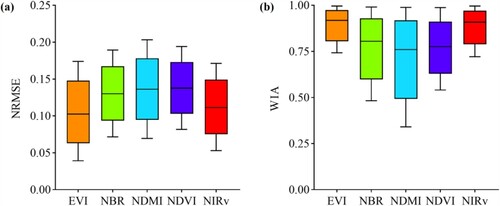
Table 2. The proportion of detected abrupt change areas using five vegetation indices, and the proportion of each index in the minimum normalized root mean square error (NRMSE) and maximum Willmott's index of agreement (WIA) (%).

Type	Region	Vegetation index
		EVI	NBR	NDMI	NDVI	NIRv
Abrupt change	Study area	58.58	60.22	66.23	61.12	66.76
	Wuyishan National Park	47.6	46.8	56.17	41.65	59.22
	Peripheral area	62.35	64.82	69.68	67.81	69.35
Minimum NRMSE	Study area	54.6	13.03	6.02	2.98	23.37
	Wuyishan National Park	53.75	16.71	3.24	1.94	24.36
	Peripheral area	54.89	11.77	6.97	3.34	23.03
Maximum WIA	Study area	57.44	11.54	4.98	2.75	23.29
	Wuyishan National Park	58.04	11.86	2.11	1.4	26.59
	Peripheral area	57.22	11.44	5.97	3.21	22.16

4.1.2. Spatial and temporal consistencies of detected abrupt changes

The completely consistent area in ALC accounted for more than 50% of the study area, with the non-changed (‘0’) and changed (‘5’) pixels accounting for 12.93% and 37.65%, respectively. The completely consistent proportion outside the park was higher than inside the park due to the higher proportion of ‘5’ outside the park (Table 3). The proportions of ‘1’, ‘2’, ‘3’, and ‘4’ were similar, but the combined proportion of ‘1’ and ‘2’ was higher than that of combined ‘3’ and ‘4’ inside the park. It was more difficult to obtain spatial consistency for change detection inside the park than outside the park. NDVI contributed more to ‘1’ and ‘2’ and contributed less to ‘4’ (Figure 7b-1). It was more difficult for NDVI to obtain consistent abrupt change-detection results than other vegetation indices. The spatial patterns of different agreement counts showed that ‘5’ was mainly distributed in the southern region of the periphery and near the eastern and western boundaries of the national park (Figure 7a-1). ‘0’ and ‘1’ were mainly distributed in the northern part of the periphery and the central part of the national park (Figure 7a-1), where vegetation was more stable with no or only one index detecting abrupt change.

Figure 7. (a-1) and (a-2) Spatial distribution of abrupt change location consistency (ALC) and abrupt time consistency (ATC). (b-1) and (b-2) Area proportion of agreement counts in ALC and ATC. The x-axes in b-1 and b-2 represent 32 different combinations of five vegetation indices. Black dots represent abrupt changes detected by the indices, and grey dots indicate no detection of abrupt changes. The numbers on the stacking histogram represent the agreement counts. The first combination in b-1 indicates no abrupt change was detected by the five indices (agreement count = 0). The tenth combination in b-2 indicates EVI and NIRv detected abrupt change in the same year (agreement count = 2) but other vegetation indices did not.

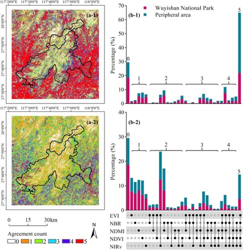
Table 3. Percentage of agreement counts of abrupt change location consistency (ALC) and time consistency (ATC) in different regions (%).

Type	Region	Agreement count
		0	1	2	3	4	5
ALC	Study area	12.93	11.6	13.04	12.11	12.67	37.65
	Wuyishan National Park	18.46	16.07	17.57	13.25	12.77	21.88
	Peripheral area	11.04	10.07	11.48	11.72	12.63	43.06
ATC	Study area	12.93	25.43	28.21	16.05	8.75	8.63
	Wuyishan National Park	18.46	33.15	27.71	11.06	5.03	4.59
	Peripheral area	11.04	22.78	28.38	17.76	10.02	10.02

The proportion of completely consistent areas in ATC was less than 25% of the study area, with the identical change year accounting for 8.63% of the study area (Table 3). ‘2’ had the highest proportion, mainly from the pairings of NDMI-NBR and EVI-NIRv (Figure 7b-2). The proportion of ATC between wetness indices and greenness indices was very low. The proportion of ‘5’ inside the park was lower than that outside the park (Figure 7a-2). When four of the five indices obtained the same change year, NDVI was not consistent with the other vegetation indices (Figure 7b-2).

4.1.3. Consistency in characterizing vegetation change trends

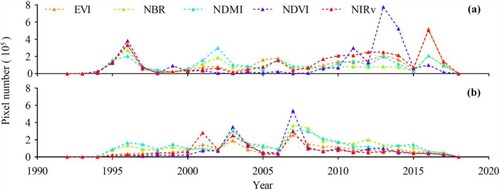
Negative abrupt change mainly occurred in 2003 and 2007, and positive abrupt change mainly occurred around 2013 and 2016. The distributions of abrupt greening and browning were similar between 1986 and 2020 for the same category of indices (except NDVI) (Figure 8). More abrupt browning pixels were detected by NBR and NDMI, and more abrupt greening pixels were detected by EVI and NIRv. NDVI was obviously different from other vegetation indices in some years (more abrupt greening in 2011, 2013, and 2014, and more abrupt browning in 2003 and 2007).

Figure 8. Number of abrupt greening and browning pixels between 1986 and 2020 (no abrupt change was detected before 1992 or after 2018). (a) abrupt greening (b) abrupt browning.

The five vegetation indices were more likely to achieve completely consistent results in CAC, CGC, and TotC than ALC and ATC. The areal proportions of all indices showing completely consistent trends for CA, CG, and Tot were 52.38%, 44.05%, and 56.10%, respectively (Table 4, Figure 9). For CA, the proportion of complete consistency outside the park (38.06%) was lower than that inside the park (43.48%). The proportions of complete consistency outside the park (47.73%, 60.73%) were higher than those inside the park (33.29%, 42.59%) for CG and Tot, respectively (Table 4, Figure 9b).

Figure 9. (a-1), (a-2), and (a-3) Spatial distribution of cumulative abrupt change consistency (CAC), cumulative gradual change consistency (CGC), and total change consistency (TotC) between 1996 and 2020. (b-1), (b-2), and (b-3) Area proportion of agreement counts in CAC, CGC, and TotC between 1986 and 2020. The x-axes represent 32 different combinations of five vegetation indices. Black dots represent the negative changes detected by the indices, while the grey dots represent the non-negative changes detected. The numbers on the stacking histogram represent the agreement counts. The first combination shows all five indices detected non-negative trends (agreement count = 0).

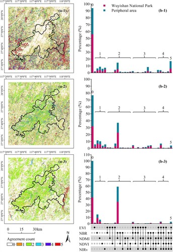
Table 4. Percentage of agreement counts of cumulative abrupt change consistency (CAC), cumulative gradual change consistency (CGC), and total change consistency (TotC) in different regions (%). The numbers in parentheses represent the area proportion of no abrupt change.

Type	Region	Agreement count
		0	1	2	3	4	5
CAC	Study area	42.64 (12.93)	15.34	14.86	10.42	7	9.74
	Wuyishan National Park	55.99 (18.46)	15.12	11.31	6.98	4.65	5.95
	Peripheral area	38.06 (11.04)	15.42	16.07	11.6	7.81	11.04
CGC	Study area	41.59	42.64 (12.93)	15.34	14.86	10.42	7
	Wuyishan National Park	32.00	55.99 (18.46)	15.12	11.31	6.98	4.65
	Peripheral area	44.86	38.06 (11.04)	15.42	16.07	11.6	7.81
TotC	Study area	54.02	54.02	10.75	28.28	2.93	1.94
	Wuyishan National Park	41.97	41.97	14.13	36.79	3.94	2.55
	Peripheral area	58.15	58.15	9.59	25.36	2.58	1.74

The wetness indices detected more negative CG with a high proportion of ‘2’ inside the park. The proportions of negative change monitored by greenness indices were relatively low (Figure 9b). When only one vegetation index monitored negative vegetation change, NDMI had the highest proportion for CA, and NBR had the highest proportions for CG and Tot (Figure 9b). When only two vegetation indices monitored negative vegetation change, the paired NDMI and NBR had the highest proportion for CA, CG, and Tot. NIRv was not consistent with other vegetation indices when four vegetation indices monitored negative CA, and NDVI was not consistent with other vegetation indices when four vegetation indices monitored negative CG (Figure 9).

4.2. Ensemble of five change-detection results

4.2.1. Accuracy assessment

The overall accuracy of abrupt vegetation change detection varied among indices, with OA ranging from 69.6% (NIRv) to 81.6% (Ensemble) (Table 5). For no change classes, the UA ranged from 89.19% (NDVI) to 98.25% (Ensemble), and PA ranged from 58.47% (NIRv) to 71.88% (Ensemble). For the change classes, the UA ranged from 55.93% (NIRv) to 67.53% (Ensemble), and PA ranged from 87.17% (EVI, NDVI) to 97.87% (Ensemble). Overall, the wetness indices performed better than the greenness indices in vegetation change detection. Compared to the spatial accuracy, the temporal accuracy significantly decreased (Table 6). The wetness indices had higher OA than greenness indices, with the highest PA in NDMI and the highest UA in NBR. The proposed ensemble algorithm had the highest accuracy both in spatial and temporal abrupt change detection.

Table 5. Accuracy assessment of change detection using five indices and the ensemble method.

VI		Reference		PA (%)	UA (%)	OA (%)
	Predicted	No change	Change
EVI	No change	225	24	71.88	90.36	77.60
	Change	88	163	87.17	64.94
NBR	No change	223	12	71.25	94.89	79.60
	Change	90	175	93.58	66.04
NDMI	No change	190	15	60.70	92.68	72.40
	Change	123	172	91.98	58.31
NDVI	No change	198	24	63.26	89.19	72.20
	Change	115	163	87.17	58.63
NIRv	No change	183	22	58.47	89.27	69.60
	Change	130	165	88.24	55.93

Table 6. Accuracy evaluation of abrupt change year.

VI	Correct Year	PA (%)	UA (%)
EVI	102	54.55	40.64
NBR	128	68.45	48.30
NDMI	136	72.73	46.10
NDVI	100	53.48	35.97
NIRv	99	52.94	33.56
Ensemble	160	85.56	59.04

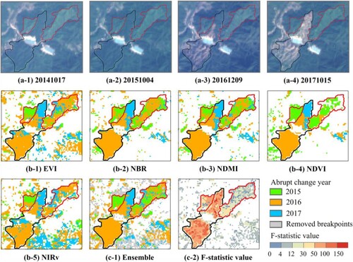
To better show how the ensemble method improved the change-detection accuracy, an example of change-detection results from each index and ensemble method are shown in Figure 10. Chow Test successfully ‘cleaned up’ the pseudo change points. The spatial distribution of breakpoints detected by EVI was similar to that of NIRv, but both indices detected a small range of false change years and some pseudo breakpoints. The spatial distribution of breakpoints detected by NBR was similar to that of NDMI. NDVI had higher omission errors and earlier detection of recovery than other vegetation indices. The boundary of two change events detected by the ensemble algorithm was clearer and more accurate (Figure 10c-1). The regions with smaller F values showed greater divergence in the change years detected by the five indices.

Figure 10. (a-1 – a-4) A logging event (black line) and a regrowth event (red line) shown in Landsat-8 images (RGB composite with red, green and blue bands) from 2014 to 2017. (b-1–b-5) The breakpoints detected by BFAST based on the five indices. (c-1) The breakpoints detected by the ensemble algorithm (combined indices). (c-2) F-statistic value.

4.2.2. Change-detection results of the ensemble algorithm

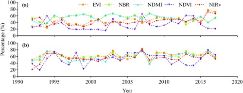
The abrupt change area detected by two or more indices accounted for 75.47% of the study area (Table 3), but the area proportion detected by the ensemble algorithm decreased to 65.41%. The wetness indices contributed more to the ensemble results than greenness indices, except in 2013, 2014, 2016, and 2017 (Figure 11a). NDVI had the lowest contribution to the ensemble results, except in 1994, 2007, 2013, and 2014. The breakpoints in each index were retained at a similar rate in most years, but breakpoints in NDVI were retained at a lower rate than other indices in 1999, 2011, 2013, and 2014 (Figure 11b).

Figure 11. (a) The area proportion of abrupt change detected by each vegetation index to the ensemble algorithm every year. (b) The proportion of retained breakpoints for each index every year.

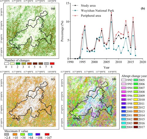
The ensemble results showed that Wuyishan National Park was well protected with fewer abrupt changes (Figure 12a). The changed area in the peripheral area was significantly higher than that in the national park after 2008, which may be related to the more strict protection measures (e.g. restricting the reclamation of Tea Mountain, completely prohibiting the clear-cutting of the natural coniferous forest) implemented in the park in 2008 (S. He and Su 2022). The abrupt change distribution showed strong synchronization during the study period (Figure 12b). The higher F-statistic values were mainly distributed in the peripheral area (Figure 12c). The most important change years show that abrupt change occurred mainly in 2003 and 2007 in western Wuyishan National Park, in 1996 and 2002 in eastern Wuyishan National Park, and in 2007 in the peripheral area (Figure 12b and d).

Figure 12. (a) Spatial distribution of abrupt change times detected by ensemble method. (b) Percentage of the changed area in different regions between 1986 and 2020 (no abrupt change was detected before 1992 and after 2018). (c) Maximum F value. (d) Spatial distribution of the most important breakpoint with maximum F value.

5. Discussion

5.1. Potential causes of the inconsistencies among different vegetation indices

The five vegetation indices showed very different fitting accuracies in the process of change detection based on BFAST. This may be the direct reason why they showed very inconsistent change-detection results on spatial and temporal scales. The breakpoint was determined by the residual sum of squares (RSS) calculated based on the fitting model in the BFAST method. The fitting errors of greenness indices were lower than those of wetness indices. One possible reason may be that the harmonic model used was not a universal function to characterize vegetation change for different vegetation indices. The greenness indices are used to extract forest phenology characterizations, such as the beginning and end of the growing seasons (Verma et al. 2016). Wetness indices have proved more useful in extracting forest disturbances (Pastor-Guzman, Dash, and Atkinson 2018). In addition, the vegetation change detection was based on the statistics of the fitted model and was difficult to relate to specific disturbance events. Exploring the relationships between forest phenology variation and disturbance processes in the spectral band would be a fruitful area of future research (Cohen et al. 2020).

Although the five indices have high spatial consistencies of detecting abrupt change, their ATC are very low. When we only pay attention to these abrupt change areas (‘5’), the spatial consistencies is low and similar to the findings of Bueno et al. (2020) in three distinct vegetation domains (Atlantic forest, savannah, and semi-arid woodland). Vegetation domains do not influence this low rate of spatial agreement (Bueno et al. 2020). NDVI is the main source of location inconsistency for abrupt change. It is easily saturated and insensitive to high-density vegetation or soil brightness conditions. The inconsistency of Landsat sensors (especially ETM and OLI) results in strong and persistent positive bias in NDVI and an offsetting effect in wetness indices and EVI (Holden and Woodcock 2016). This may be why NDVI detected more positive abrupt changes that were not detected by other indices in 2013.

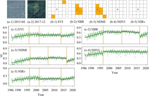
The ‘2’ and ‘3’ were largely due to the similar abrupt change time detected by the same category (greenness or wetness), but significantly differed between different categories of vegetation indices. Wetness indices use the SWIR band and have shown to be more sensitive to a variety of disturbance types compared to greenness indices and were less affected by atmospheric water vapor and aerosols (Grogan et al. 2016). Secondary vegetation can quickly recover, which leads to a rapid saturation of NIR/red values that respond to chlorophyll presence and leaf area index after a logging event occurs. This effect can reduce the sensitivity of greenness indices to forest change (Smith et al. 2019). Figure 13 illustrates a small-scale logging event in 2016. The wetness indices were able to detect this event, while the greenness indices were not due to the quick recovery of chlorophyll and leaf area index.

Figure 13. A small-scale logging event. (a-1) and (a-2) in Google Earth in April 2015 and December 2017, respectively. (b-1–b-5) represent the vegetation change-detection results of five indices, with yellow representing abrupt changes detected in 2016. (c-1–c-5) represent the breakpoint detection of the pixel marked with an asterisk, with grey dots representing the actual observations from 1986 to 2020, the black lines representing change trends (gradual change), the green curves representing harmonic model, and the yellow lines representing the dates of the detected breakpoints.

Anthropogenic disturbances lead to consistent change detection results, but some specific minor disturbances do not. Anthropogenic disturbances are more likely to cause large change magnitude in very short time, while natural disturbances are more likely cause subtle changes. Completely consistent (‘0’ and ‘5’) area proportions of ALC and ATC are higher outside the park than inside the park. This resulted from the different disturbance patterns with natural disturbance dominating inside the park and anthropogenic disturbance dominating outside the park (Yang and Xu 2020). Natural disturbances affect the forest environment and change the forest structure and function, thus becoming one of the driving forces of forest ecosystem succession/change (Wang et al. 2003). Extreme disturbance (drought, snow disaster, etc.) caused great changes in the forest canopy, individual trees, soil surface structure, soil nutrition, and physical and chemical properties, thus changing the forest species structure, whereas weak natural disturbances (windfall, pests, climate change, etc.) may promote the regeneration of multiple species and mechanisms (Liang, Wang, and Liang 2002). Minor natural disturbance and succession are slow processes in which the biophysical parameters of plants change at different times (Assal, Anderson, and Sibold 2016; Piragnolo et al. 2021), making it difficult for the five indices to respond uniformly to them. Anthropogenic disturbance (urbanization construction, road expansion, tea field reclamation, tourism, etc.) directly changes the forest landscape, as shown in Figure 10. It should be noted that the definition of completely consistent is somewhat subjective. For example, it can be a consistent result if the wetness indices show a decrease in moisture due to a drought and greenness indices do not. However, the percentage of such consistent result was low in the study area (Figure 7).

The vegetation changes CAC, CGC, and TotC showed higher consistencies between the wetness and greenness than ALC and ATC. Five vegetation indices increased universally in the study area, but some regions showed obvious inconsistencies with decreased wetness indices and increased greenness indices, which was also observed in a natural forest of inner north-eastern Spain dominated by P. pinaster (Moreno-Fernández et al. 2021), and in Arctic Lena Delta dominated by sedge, grass, moss and dwarf shrub wetlands (Nitze and Grosse 2016). Although the two studies conducted in different ecosystems with ours, they both used dense Landsat time series data and focused on vegetation change trend analysis. The inconsistent regions were mainly distributed on the western and north-western slopes. Vegetation response to water stress is influenced by factors such as vegetation functional type and climatic conditions (Moreno-Fernández et al. 2021). Aspect may affect the consistency of gradual versus abrupt change. The temperature has gradually increased and precipitation has gradually decreased in recent decades (Liu et al. 2022), and the hydrothermal conditions on the east slope are better than those on the west slope in the study area (Zou 2014). Forest stands with higher canopy cover and density on the west slope of the park would likely be more water-stressed. In addition, the water-use strategies of different tree species can also explain the apparent decreasing trend of wetness. Broadleaves can use the water stored in the heartwood during prolonged dry periods, whereas conifers keep their water reserves mainly by real-time absorption (Querejeta et al. 2007; Goldsmith 2013).

5.2. Improvement of change detection

Our study showed that PA was higher than UA for the changed class and UA was higher than PA for the non-changed class at spatial scale. Five VIs all overestimate changes, which is similar to the finding of Schultz et al. (2016). Wetness indices outperformed greenness indices in characterizing abrupt vegetation change at temporal scale. The greater contribution of the wetness indices to the ensemble results in our study also indicated that wetness indices were more effective for disturbance detection. These findings are consistent with Cohen et al. (2020, 2018), DeVries et al. (2015), Schultz et al. (2016), and Smith et al. (2019). The SWIR band and SWIR-based indices had the highest median DSNR (change signal-to-noise ratio), and the use of the SWIR band or SWIR-based indices is the most important consideration when using a single spectral dimension for vegetation disturbance detection in U.S. forests (Cohen et al. 2018).

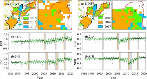
The ensemble method had higher accuracy than any single-index change detection at spatial and temporal scales. This gain of multiple spectral indices in the ensemble method is supported by the different responses of spectral indices for disturbance events (Hislop et al. 2018; Schultz et al. 2016; Shimizu et al. 2019), and the removal of false breakpoints (Bullock, Woodcock, and Holden 2020). An example in Figure 14 showed the added value of the greenness index in final ensemble change detection. Locations A and B are adjacent to each other and experienced similar changes. Location A experienced a subtler abrupt change in 2016 than location B, and the change was detected by EVI but ignored in NBR (Figure 14 b-1 and b-2). The abrupt change at location B was detected by both EVI and NBR (Figure 14 b-3 and b-4). The ensemble algorithm retained the two abrupt changes at these two locations. The greenness index was more sensitive to positive abrupt changes, while the wetness index was more sensitive to negative abrupt change. The wetness index detected a cutting event occurred in 2011 (Figure 14b-4) and greenness index detected a positive abrupt change due to the rapid recovery of chlorophyll and leaf area index after one year (2012) (Figure 14 b-3). The synergetic greenness-wetness content strategy possesses advantages to capture and characterize the subtle variations in the canopy components (Liu et al. 2021). However, this gain is relatively small, and the ensemble algorithm does not overcome the disadvantage of the BFAST algorithm, which cannot detect breakpoints at the beginning and end of the time series. This ensemble method may be expected to translate directly to other places with low accessibility and cloudy and rainy conditions.

Figure 14. (a-1) and (a-2) are from Figure 10. (b-1), (b-2), (b-3) and (b-4) EVI and NBR time series for a pixel labelled in (a-1) and (a-2) as ‘A’ and ‘B’ with abrupt change detected by BFAST, respectively. Grey points represent the actual observations from 1986 to 2020, green curves represent values fitted by harmonic models, black lines represent gradual changes, yellow lines represent the dates of the breakpoints detected by BFAST, and grey rectangles represent the dates of breakpoints detected by the ensemble algorithm with a backward 1-year window.

5.3. Limitations

Abrupt change is defined rather ambiguously in the time-series remote sensing data and leaves substantial room for interpretation. Abrupt change has often been related to the term disturbance; however, they have different meanings according to different change-detection tasks and ecosystems. The validation data from manual interpretation are also hard to align with the definitions built into the algorithm and real disturbance events. For example, the stand-replacing disturbance can be recognized in most conditions, but subtle changes are easily missed in both algorithm and manual interpretation. It is important to define disturbance priority with field experiments, which is the best basis to improve change-detection accuracies.

6. Conclusion

Quantifying where and when the commonly used vegetation indices have consistent and inconsistent change-detection results is fundamental to investigating the drivers and mechanisms of vegetation change. Analysis of vegetation change and response to climate change based on a single indicator may lead to high uncertainties due to the high inconsistency in detecting vegetation changes. This study evaluated the differences of five Landsat vegetation indices (EVI, NDVI, NIRv, NBR, and NDMI) in detecting spatial and temporal abrupt vegetation change, and vegetation change trends. NDVI is the main source of disagreement among the five indices in abrupt change detection. It should be carefully used and compared with other vegetation indices, especially using both Landsat 8 and Landsat 5/7 data. Wetness indices (NBR, NDMI) detected more abrupt changes with browning change, and greenness indices (EVI, NDVI, NIRv) detected more abrupt changes with greening change. Wetness and greenness indices are very similar in detecting gradual and total vegetation change. Wetness indices (NBR, NDMI) perform better than greenness indices (EVI, NDVI, NIRv) in the abrupt change detection. NBR had the highest accuracy (79.6%) in abrupt change detection among the five vegetation indices. The proposed ensemble method based on abrupt change detection results of five vegetation indices can further increase change-detection accuracy without high quality reference data training. It can be easily applied in larger regions across multiple vegetation domains. This study provided a thorough evaluation of the inconsistencies among different vegetation indices from model fitting, change detection, and vegetation change trends. We further proposed an ensemble method to combine the change results to improve the accuracy of the change-detection result.

Disclosure statement

No potential conflict of interest was reported by the author(s).

Data availability statement

The data that support the findings of this study are available from the corresponding author upon reasonable request.

Additional information

Funding

This work was supported by Natural Science Foundation of Fujian Province [grant number 2022J01640, 2022J011076], Public welfare projects of Fujian Provincial Science and Technology Department [grant number 2021R1002008], and National Natural Science Foundation of China [grant number 41701490].

References

- Abdullah, Nor Azliana, Nasrudin Abd Rahim, Chin Kim Gan, and Noriah Nor Adzman. 2019. “Forecasting Solar Power Using Hybrid Firefly and Particle Swarm Optimization (HFPSO) for Optimizing the Parameters in a Wavelet Transform-Adaptive Neuro Fuzzy Inference System (WT-ANFIS).” Applied Sciences (Switzerland) 9 (16): 3214. doi:10.3390/app9163214.
- Assal, Timothy J., Patrick J. Anderson, and Jason Sibold. 2016. “Spatial and Temporal Trends of Drought Effects in a Heterogeneous Semi-Arid Forest Ecosystem.” Forest Ecology and Management 365: 137–151. doi:10.1016/j.foreco.2016.01.017.
- Awty-Carroll, Katie, Pete Bunting, Andy Hardy, and Gemma Bell. 2019. “An Evaluation and Comparison of Four Dense Time Series Change Detection Methods Using Simulated Data.” Remote Sensing 11 (23): 2779. doi:10.3390/rs11232779.
- Badgley, Grayson, Christopher B. Field, and Joseph A. Berry. 2017. “Canopy Near-Infrared Reflectance and Terrestrial Photosynthesis.” Science Advances 3 (3): e1602244. doi:10.1126/sciadv.1602244.
- Berner, Logan T., and Scott J. Goetz. 2022. “Satellite Observations Document Trends Consistent with a Boreal Forest Biome Shift.” Global Change Biology, doi:10.1111/gcb.16121.
- Bonan, Gordon B., David Pollard, and Starley L. Thompson. 1992. “Effects of Boreal Forest Vegetation on Global Climate.” Nature 359 (6397): 716–718. doi:10.1038/359716a0.
- Bueno, Inacio T., Greg J. McDermid, Eduarda M.O. Silveira, Jennifer N. Hird, Breno I. Domingos, and Fausto W. Acerbi Júnior. 2020. “Spatial Agreement among Vegetation Disturbance Maps in Tropical Domains Using Landsat Time Series.” Remote Sensing 12), doi:10.3390/RS12182948.
- Bullock, Eric L., Curtis E. Woodcock, and Christopher E. Holden. 2020. “Improved Change Monitoring Using an Ensemble of Time Series Algorithms.” Remote Sensing of Environment 238: 111165. doi:10.1016/j.rse.2019.04.018.
- Cohen, Warren B., Sean P. Healey, Zhiqiang Yang, Zhe Zhu, and Noel Gorelick. 2020. “Diversity of Algorithm and Spectral Band Inputs Improves Landsat Monitoring of Forest Disturbance.” Remote Sensing 12 (10): 1673. doi:10.3390/rs12101673.
- Cohen, Warren B., Zhiqiang Yang, Sean P. Healey, Robert E. Kennedy, and Noel Gorelick. 2018. “A LandTrendr Multispectral Ensemble for Forest Disturbance Detection.” Remote Sensing of Environment 205: 131–140. doi:10.1016/j.rse.2017.11.015.
- Cohen, Warren B., Zhiqiang Yang, and Robert Kennedy. 2010. “Detecting Trends in Forest Disturbance and Recovery Using Yearly Landsat Time Series: 2. TimeSync — Tools for Calibration and Validation.” Remote Sensing of Environment 114 (12): 2911–2924. doi:10.1016/j.rse.2010.07.010.
- De Jong, Rogier, Jan Verbesselt, Michael E. Schaepman, and Sytze de Bruin. 2012. “Trend Changes in Global Greening and Browning: Contribution of Short-Term Trends to Longer-Term Change.” Global Change Biology 18 (2): 642–655. doi:10.1111/j.1365-2486.2011.02578.x.
- DeVries, Ben, Mathieu Decuyper, Jan Verbesselt, Achim Zeileis, Martin Herold, and Shijo Joseph. 2015a. “Tracking Disturbance-Regrowth Dynamics in Tropical Forests Using Structural Change Detection and Landsat Time Series.” Remote Sensing of Environment 169: 320–334. doi:10.1016/j.rse.2015.08.020.
- DeVries, Ben, Jan Verbesselt, Lammert Kooistra, and Martin Herold. 2015b. “Robust Monitoring of Small-Scale Forest Disturbances in a Tropical Montane Forest Using Landsat Time Series.” Remote Sensing of Environment 161: 107–121. doi:10.1016/j.rse.2015.02.012.
- Ding, Z., J. Peng, S. Qiu, and Y. Zhao. 2020. “Nearly Half of Global Vegetated Area Experienced Inconsistent Vegetation Growth in Terms of Greenness, Cover, and Productivity.” Earth's Future 8 (10): 1–15. doi:10.1029/2020EF001618.
- Dutrieux, Loïc P., Catarina C. Jakovac, Siti H. Latifah, and Lammert Kooistra. 2016. “Reconstructing Land use History from Landsat Time-Series.” International Journal of Applied Earth Observation and Geoinformation 47: 112–124. doi:10.1016/j.jag.2015.11.018.
- Esteban, Jessica, Alfredo Fernández-Landa, José Luis Tomé, Cristina Gómez, and Miguel Marchamalo. 2021. “Identification of Silvicultural Practices in Mediterranean Forests Integrating Landsat Time Series and a Single Coverage of Als Data.” Remote Sensing 13 (18): 3611. doi:10.3390/rs13183611.
- Fan, Mengzhuo, Kuo Liao, Dengsheng Lu, and Dengqiu Li. 2022. “Examining Vegetation Change and Associated Spatial Patterns in Wuyishan National Park at Different Protection Levels.” Remote Sensing 14 (7): 1712–1720. doi:10.3390/rs14071712.
- Fang, Xiuqin, Qiuan Zhu, Liliang Ren, Huai Chen, Kai Wang, and Changhui Peng. 2018. “Large-Scale Detection of Vegetation Dynamics and Their Potential Drivers Using MODIS Images and BFAST: A Case Study in Quebec, Canada.” Remote Sensing of Environment 206 (November 2017): 391–402. doi:10.1016/j.rse.2017.11.017.
- García, M. J.López, and V. Caselles. 1991. “Mapping Burns and Natural Reforestation Using Thematic Mapper Data.” Geocarto International 6 (1): 31–37. doi:10.1080/10106049109354290.
- Goldsmith, G. R. 2013. “Changing Directions: The Atmosphere–Plant–Soil Continuum.” New Phytologist 199 (1): 4–6. doi:10.1111/nph.12332.
- Grogan, Kenneth, Dirk Pflugmacher, Patrick Hostert, Jan Verbesselt, and Rasmus Fensholt. 2016. “Mapping Clearances in Tropical Dry Forests Using Breakpoints, Trend, and Seasonal Components from Modis Time Series: Does Forest Type Matter?” Remote Sensing 8 (8): 657. doi:10.3390/rs8080657.
- Haberl, Helmut, K. Heinz Erb, Fridolin Krausmann, Veronika Gaube, Alberte Bondeau, Christoph Plutzar, Simone Gingrich, Wolfgang Lucht, and Marina Fischer-Kowalski. 2007. “Quantifying and Mapping the Human Appropriation of Net Primary Production in Earth’s Terrestrial Ecosystems.” Proceedings of the National Academy of Sciences 104 (31): 12942–12947. doi:10.1073/pnas.0704243104.
- He, Siyuan, and Yang Su. 2022. “Understanding Residents’ Perceptions of the Ecosystem to Improve Park–People Relationships in Wuyishan National Park, China.” Land 11 (4): 532. doi:10.3390/land11040532.
- He, Panxing, Zongjiu Sun, Zhiming Han, Yiqiang Dong, Huixia Liu, Xiaoyu Meng, and Jun Ma. 2021. “Dynamic Characteristics and Driving Factors of Vegetation Greenness Under Changing Environments in Xinjiang, China.” Environmental Science and Pollution Research 28 (31): 42516–42532. doi:10.1007/s11356-021-13721-z.
- Hislop, Samuel, Simon Jones, Mariela Soto-Berelov, Andrew Skidmore, Andrew Haywood, and Trung H. Nguyen. 2018. “Using Landsat Spectral Indices in Time-Series to Assess Wildfire Disturbance and Recovery.” Remote Sensing 10 (3): 460. doi:10.3390/rs10030460.
- Hislop, Samuel, Simon Jones, Mariela Soto-Berelov, Andrew Skidmore, Andrew Haywood, and Trung H. Nguyen. 2019. “A Fusion Approach to Forest Disturbance Mapping Using Time Series Ensemble Techniques.” Remote Sensing of Environment 221: 188–197. doi:10.1016/j.rse.2018.11.025.
- Holden, Christopher E., and Curtis E. Woodcock. 2016. “An Analysis of Landsat 7 and Landsat 8 Underflight Data and the Implications for Time Series Investigations.” Remote Sensing of Environment 185: 16–36. doi:10.1016/j.rse.2016.02.052.
- Huete, A., K. Didan, T. Miura, E. P. Rodriguez, X. Gao, and L. G. Ferreira. 2002. “Overview of the Radiometric and Biophysical Performance of the MODIS Vegetation Indices.” Remote Sensing of Environment 83 (1–2): 195–213. doi:10.1016/S0034-4257(02)00096-2.
- Kennedy, Robert E., Zhiqiang Yang, and Warren B. Cohen. 2010. “Detecting Trends in Forest Disturbance and Recovery Using Yearly Landsat Time Series: 1. LandTrendr — Temporal Segmentation Algorithms.” Remote Sensing of Environment 114 (12): 2897–2910. doi:10.1016/j.rse.2010.07.008.
- Kulawardhana, Ranjani Wasantha. 2011. “Remote Sensing of Vegetation: Principles, Techniques and Applications. By Hamlyn G. Jones and Robin A Vaughan.” Journal of Vegetation Science 22 (6): 1151–1153. doi:10.1111/j.1654-1103.2011.01319.x.
- Li, Dengqiu, Dengsheng Lu, Ming Wu, Xuexin Shao, and Jinhong Wei. 2018. “Examining Land Cover and Greenness Dynamics in Hangzhou Bay in 1985-2016 Using Landsat Time-Series Data.” Remote Sensing 10 (1): 32. doi:10.3390/rs10010032.
- Li, Dengqiu, Dengsheng Lu, Yan Zhao, Mingxing Zhou, and Guangsheng Chen. 2021. “Spatial Patterns of Vegetation Coverage Change in Giant Panda Habitat Based on MODIS Time-Series Observations and Local Indicators of Spatial Association.” Ecological Indicators 124: 107418. doi:10.1016/j.ecolind.2021.107418.
- Liang, Jianping, Aiming Wang, and Shengfa Liang. 2002. “Disturbance and Forest Regeneration.” Forest Research 15 (4): 590–498. doi:10.13275/j.cnki.lykxyj.2002.04.023. In Chinese.
- Lin, Sen, Xisheng Hu, Chengzhen Wu, and Wei Hong. 2020. “Temporal-Spatial Features of Vegetation Cover in Mount Wuyi National Park.” Journal of Forest and Environment 40 (4): 347–355. doi:10.13324/j.cnki.jfcf.2020.04.002. In Chinese.
- Liu, Feng, Hongyan Liu, Chongyang Xu, Liang Shi, Xinrong Zhu, Yang Qi, and Wenqi He. 2021. “Old-Growth Forests Show low Canopy Resilience to Droughts at the Southern Edge of the Taiga.” Global Change Biology 27 (11): 2392–2402. doi:10.1111/gcb.15605.
- Liu, Yue, Yihan Pu, Yanqing Liu, Deshuai An, Dandan Xu, Jianqin Zhu, and Honghua Ruan. 2022. “Study on the Impact of Global Climate Change on the Communities of Vegetation Vertical Zone Spectrum in Wuyishan National Park Based on Landsat Imagery.” Ecological Science 41 (5): 152–162. doi:10.14108/j.cnki.1008-8873.2022.05.019. In Chinese.
- Masek, Jeffrey G., Eric F. Vermote, Nazmi E. Saleous, Robert Wolfe, Forrest G. Hall, Karl F. Huemmrich, Feng Gao, Jonathan Kutler, and Teng Kui Lim. 2006. “A Landsat Surface Reflectance Dataset for North America, 1990-2000.” IEEE Geoscience and Remote Sensing Letters 3 (1): 68–72. doi:10.1109/LGRS.2005.857030.
- Matsushita, Bunkei, Wei Yang, Jin Chen, Yuyichi Onda, and Guoyu Qiu. 2007. “Sensitivity of the Enhanced Vegetation Index (EVI) and Normalized Difference Vegetation Index (NDVI) to Topographic Effects: A Case Study in High-Density Cypress Forest.” Sensors 7 (11): 2636–2651. doi:10.3390/s7112636.
- Mayer, D. G., and D. G. Butler. 1993. “Statistical Validation.” Ecological Modelling 68 (1–2): 21–32. doi:10.1016/0304-3800(93)90105-2.
- Moreno-Fernández, Daniel, Alba Viana-Soto, Julio Jesús Camarero, Miguel A. Zavala, Julián Tijerín, and Mariano García. 2021. “Using Spectral Indices as Early Warning Signals of Forest Dieback: The Case of Drought-Prone Pinus Pinaster Forests.” Science of the Total Environment 793: 148578. doi:10.1016/j.scitotenv.2021.148578.
- Murillo-Sandoval, Paulo J., Thomas Hilker, Meg A. Krawchuk, and Jamon Van Den Hoek. 2018. “Detecting and Attributing Drivers of Forest Disturbance in the Colombian Andes Using Landsat Time-Series.” Forests 9 (5): 269. doi:10.3390/f9050269.
- Nitze, Ingmar, and Guido Grosse. 2016. “Detection of Landscape Dynamics in the Arctic Lena Delta with Temporally Dense Landsat Time-Series Stacks.” Remote Sensing of Environment 181: 27–41. doi:10.1016/j.rse.2016.03.038.
- Pastor-Guzman, J., Jadunandan Dash, and Peter M. Atkinson. 2018. “Remote Sensing of Mangrove Forest Phenology and Its Environmental Drivers.” Remote Sensing of Environment 205: 71–84. doi:10.1016/j.rse.2017.11.009.
- Piragnolo, Marco, Francesco Pirotti, Carlo Zanrosso, Emanuele Lingua, and Stefano Grigolato. 2021. “Responding to Large-Scale Forest Damage in an Alpine Environment with Remote Sensing, Machine Learning, and Web-GIS.” Remote Sensing 13, doi:10.3390/rs13081541.
- Querejeta, José, Héctor Ignacio, Michael F. Estrada-Medina, and Juan José Jiménez-Osornio. Allen. 2007. “Water Source Partitioning among Trees Growing on Shallow Karst Soils in a Seasonally Dry Tropical Climate.” Oecologia 152 (1): 26–36. doi:10.1007/s00442-006-0629-3.
- Rouse, J. W., R. H. Hass, J. A. Schell, and D. W. Deering. 1976. “Metabolism of Limonoids. Limonin D-Ring Lactone Hydrolase Activity in Pseudomonas.” Journal of Agricultural and Food Chemistry 24 (1): 24–26. doi:10.1021/jf60203a024.
- Saxena, Rishu, Layne T. Watson, Valerie A. Thomas, and Randolph H. Wynne. 2017. “Scaling Constituent Algorithms of a Trend and Change Detection Polyalgorithm.” Simulation Series 49 (3): 59–70. doi:10.22360/springsim.2017.hpc.020.
- Schroeder, Todd A., Michael A. Wulder, Sean P. Healey, and Gretchen G. Moisen. 2011. “Mapping Wildfire and Clearcut Harvest Disturbances in Boreal Forests with Landsat Time Series Data.” Remote Sensing of Environment 115 (6): 1421–1433. doi:10.1016/j.rse.2011.01.022.
- Schultz, Michael, Jan G.P.W. Clevers, Sarah Carter, Jan Verbesselt, Valerio Avitabile, Hien Vu Quang, and Martin Herold. 2016. “Performance of Vegetation Indices from Landsat Time Series in Deforestation Monitoring.” International Journal of Applied Earth Observation and Geoinformation 52: 318–327. doi:10.1016/j.jag.2016.06.020.
- Schultz, Michael, Aurélie Shapiro, Jan G.P.W. Clevers, Craig Beech, and Martin Herold. 2018. “Forest Cover and Vegetation Degradation Detection in the Kavango Zambezi Transfrontier Conservation Area Using BFAST Monitor.” Remote Sensing 10 (11): 1850. doi:10.3390/rs10111850.
- Shimizu, Katsuto, Tetsuji Ota, Nobuya Mizoue, and Shigejiro Yoshida. 2019. “A Comprehensive Evaluation of Disturbance Agent Classification Approaches: Strengths of Ensemble Classification, Multiple Indices, Spatio-Temporal Variables, and Direct Prediction.” ISPRS Journal of Photogrammetry and Remote Sensing 158: 99–112. doi:10.1016/j.isprsjprs.2019.10.004.
- Smith, Vaughn, Carlos Portillo-Quintero, Arturo Sanchez-Azofeifa, and Jose L. Hernandez-Stefanoni. 2019. “Assessing the Accuracy of Detected Breaks in Landsat Time Series as Predictors of Small Scale Deforestation in Tropical Dry Forests of Mexico and Costa Rica.” Remote Sensing of Environment 221: 707–721. doi:10.1016/j.rse.2018.12.020.
- Tucker, Compton J. 1979. “Red and Photographic Infrared Linear Combinations for Monitoring Vegetation.” Remote Sensing of Environment 8 (2): 127–150. doi:10.1016/0034-4257(79)90013-0.
- Verbesselt, Jan, Rob Hyndman, Glenn Newnham, and Darius Culvenor. 2010. “Detecting Trend and Seasonal Changes in Satellite Image Time Series.” Remote Sensing of Environment 114 (1): 106–115. doi:10.1016/j.rse.2009.08.014.
- Verbesselt, Jan, Rob Hyndman, Achim Zeileis, and Darius Culvenor. 2010. “Phenological Change Detection While Accounting for Abrupt and Gradual Trends in Satellite Image Time Series.” Remote Sensing of Environment 114 (12): 2970–2980. doi:10.1016/j.rse.2010.08.003.
- Verma, Manish, Mark A. Friedl, Adrien Finzi, and Nathan Phillips. 2016. “Multi-Criteria Evaluation of the Suitability of Growth Functions for Modeling Remotely Sensed Phenology.” Ecological Modelling 323: 123–132. doi:10.1016/j.ecolmodel.2015.12.005.
- Vermote, Eric, Chris Justice, Martin Claverie, and Belen Franch. 2016. “Preliminary Analysis of the Performance of the Landsat 8/OLI Land Surface Reflectance Product.” Remote Sensing of Environment, 46–56. doi:10.1016/j.rse.2016.04.008.
- Vogelmann, James E., and Barrett N. Rock. 1988. “Assessing Forest Damage in High-Elevation Coniferous Forests in Vermont and New Hampshire Using Thematic Mapper Data.” Remote Sensing of Environment 24 (2): 227–246. doi:10.1016/0034-4257(88)90027-2.
- Wang, Xugao, Xiuzhen Li, Fanhua Kong, Yuehui Li, Binglu Shi, and Zhenling Gao. 2003. “Model of Vegetation Restoration Under Natural Regeneration and Human Interference in the Burned Area of Northern Daxinganling.” Chinese Journal of Ecology 22 (5): 30–34. doi:10.13292/j.1000-4890.2003.0101. In Chinese.
- Willmott, Cort J. 1981. “On the Validation of Models.” Physical Geography 2 (2): 184–194. doi:10.1080/02723646.1981.10642213.
- Wu, Ling, Zhaoliang Li, Xiangnan Liu, Lihong Zhu, Yibo Tang, Biyao Zhang, Boliang Xu, Meiling Liu, Yuanyuan Meng, and Boyuan Liu. 2020. “Multi-Type Forest Change Detection Using BFAST and Monthly Landsat Time Series for Monitoring Spatiotemporal Dynamics of Forests in Subtropical Wetland.” Remote Sensing 12 (2): 341. doi:10.3390/rs12020341.
- Xin, Qinchuan, Jing Li, Ziming Li, Yaoming Li, and Xuewen Zhou. 2020. “Evaluations and Comparisons of Rule-Based and Machine-Learning-Based Methods to Retrieve Satellite-Based Vegetation Phenology Using MODIS and USA National Phenology Network Data.” International Journal of Applied Earth Observation and Geoinformation 93: 102189. doi:10.1016/j.jag.2020.102189.
- Yang, Huiting, and Hanqiu Xu. 2020. “Assessing Fractional Vegetation Cover Changes and Ecological Quality of the Wuyi Mountain National Nature Reserve Based on Remote Sensing Spatial Information.” Chinese Journal of Applied Ecology 31 (2): 533–542. doi:10.13287/j.1001-9332.202002.014. In Chinese.
- Zeileis, Achim, Friedrich Leisch, Kurt Hornik, and Christian Kleiber. 2002. “Strucchange: An R Package for Testing for Structural Change in Linear Regression Models.” Journal of Statistical Software 7: 1–38. doi:10.18637/jss.v007.i02.
- Zeng, Yelu, Dalei Hao, Alfredo Huete, Benjamin Dechant, Joe Berry, Jing M. Chen, Joanna Joiner, et al. 2022. “Optical Vegetation Indices for Monitoring Terrestrial Ecosystems Globally.” Nature Reviews Earth & Environment 3: 477–493. doi:10.1038/s43017-022-00298-5.
- Zhu, Zhe, Yingchun Fu, Curtis E. Woodcock, Pontus Olofsson, James E. Vogelmann, Christopher Holden, Min Wang, Shu Dai, and Yang Yu. 2016. “Including Land Cover Change in Analysis of Greenness Trends Using All Available Landsat 5, 7, and 8 Images: A Case Study from Guangzhou, China (2000–2014).” Remote Sensing of Environment 185: 243–257. doi:10.1016/j.rse.2016.03.036.
- Zhu, Zhe, and Curtis E. Woodcock. 2012. “Object-Based Cloud and Cloud Shadow Detection in Landsat Imagery.” Remote Sensing of Environment 118: 83–94. doi:10.1016/j.rse.2011.10.028.
- Zhu, Zhe, and Curtis E. Woodcock. 2014. “Continuous Change Detection and Classification of Land Cover Using All Available Landsat Data.” Remote Sensing of Environment 144: 152–171. doi:10.1016/j.rse.2014.01.011.
- Zhu, Yaohui, Chunjiang Zhao, Hao Yang, Guijun Yang, Liang Han, Zhenhai Li, Haikuan Feng, Bo Xu, Jintao Wu, and Lei Lei. 2019. “Estimation of Maize Above-Ground Biomass Based on Stem-Leaf Separation Strategy Integrated with LiDAR and Optical Remote Sensing Data.” PeerJ 2019 (9): e7593. doi:10.7717/peerj.7593.
- Zou, Weicheng. 2014. “Spatial Heterogeneity Relationship of Vegetation and Environmental Factors in Wuyi Mountain.” Master's Thesis, Fuzhou University. (In Chinese).