Machine learning-based prediction of sand and dust storm sources in arid Central Asia

ABSTRACT

With the emergence of multisource data and the development of cloud computing platforms, accurate prediction of event-scale dust source regions based on machine learning (ML) methods should be considered, especially accounting for the temporal variability in sample and predictor variables. Arid Central Asia (ACA) is recognized as one of the world’s primary potential sand and dust storm (SDS) sources. In this study, based on the Google Earth Engine (GEE) platform, four ML methods were used for SDS source prediction in ACA. Fourteen meteorological and terrestrial factors were selected as influencing factors controlling SDS source susceptibility and applied in the modeling process. Generally, the results revealed that the random forest (RF) algorithm performed best, followed by the gradient boosting tree (GBT), maximum entropy (MaxEnt) model and support vector machine (SVM). The Gini impurity index results of the RF model indicated that the wind speed played the most important role in SDS source prediction, followed by the normalized difference vegetation index (NDVI). This study could facilitate the development of programs to reduce SDS risks in arid and semiarid regions, particularly in ACA.

KEYWORDS:

• Susceptibility mapping
• event scale
• google earth engine (GEE)
• remote sensing

1. Introduction

As one of the most important consequences of wind erosion, sand and dust storms (SDSs) often occur in semiarid and arid regions, such as North Africa, the Middle East, and Central Asia (Youlin, Squires, and Qi 2002; Doronzo et al. 2016; Labban and Butt 2021). The most significant impact of SDSs is the threat to human health caused by the increased concentration of suspended particulate matter in the atmosphere (Wu et al. 2021). Additionally, SDSs significantly impact transportation, infrastructure, agriculture, ecosystems, climate change, etc. (Schepanski 2018; Opp et al. 2021; Jilili, Liu, and Wu 2010). Due to the destructive and significant impacts of SDSs, many studies have been devoted to accurately identifying and predicting SDS source areas to improve disaster preparedness and damage prevention (Gholami et al. 2021; Darvishi Boloorani et al. 2022; Boroughani et al. 2021). Hosseini Dehshiri et al. (2022) used the Hybrid Single-Particle Lagrangian Integrated Trajectory (HYSPLIT) model and trajectory cluster analysis to identify the main dust transport pathways and critical dust sources in central Iran. Although models are considered important in SDS identification, it remains difficult to predict SDS sources (Knippertz and Todd 2012; Darmenova et al. 2009; Huang et al. 2013; Butt and Mashat 2018; Butt, Assiri, and Alghamdi 2023). SDS outbreaks depend not only on meteorological factors such as wind speed, precipitation, and air temperature but also on terrestrial factors such as vegetation cover, snow cover, and soil characteristics (soil moisture, soil temperature, etc.) (Papi et al. 2022; Jiao et al. 2021). However, the integration of multiple remote sensing (RS) and meteorological data with different spatial and temporal resolutions and their application in SDS source prediction should be resolved (Rayegani et al. 2020). Given their notable data integration capabilities, machine learning (ML) methods are widely used in various data science fields such as identification, classification, prediction, regression, and clustering. (Liakos et al. 2018; Holloway and Mengersen 2018).

Recently, ML methods have also been extensively employed in SDS source prediction or susceptibility mapping. Lary et al. (2016) first demonstrated the promising development of machine learning algorithms (MLAs) for SDS source classification and identification. Nabavi et al. (2018) introduced five MLAs (multilinear regression (MLR), random forest (RF), multivariate adaptive regression splines (MARS), support vector machine (SVM), and artificial neural network (ANN)) for aerosol optical depth (AOD) prediction in West Asia. Gholami, Mohamadifar, et al. (2020a) applied six MLAs (eXtreme Gradient Boosting (XGBoost), Cubist, boosting multivariate adaptive regression splines (BMARS), adaptive network-based fuzzy inference system (ANFIS), Cforest and Elasticnet) to investigate the land susceptibility to dust emissions in southeastern Iran. Gholami et al. (2021) introduced a new integrated ML-based approach for the generation of spatial maps of dust sources and assessment of the interpretability of spatial maps over Central Asia. Although an increasing number of ML-based methods and even deep learning (DP)-based methods have been applied in SDS source prediction, few studies have focused on SDS source prediction at the event scale (Jiao et al. 2021). Most previous studies involved the use of averaged datasets to predict the general spatial distribution of SDS sources, which has implications for desertification control, but SDS sources are also characterized by spatial and temporal variability (Rahmati et al. 2020; Shi et al. 2020). To accurately forecast dust storms, knowledge of the spatiotemporal characteristics of SDS sources is crucial. At the same time, event-scale SDS source prediction challenges the training sample selection process at the model training stage and the consideration of input data (Jiao et al. 2021). Although there are sufficient training samples, the lack of large-scale spatiotemporal heterogeneity in the samples leads to uncertain prediction results. In most existing studies, the input data were processed as averaged images instead of image collection (IC) data, resulting in the prediction results only reflecting the spatial characteristics of the considered SDS source (Rahmati et al. 2020). A large amount of hourly-, daily- and monthly-scale input datasets for classifier training purposes is the key to solving this problem (Yu et al. 2020). Additionally, integrating publicly available multisource data (i.e. RS data, meteorological data, and soil property data) to predict SDS source distributions provides potential applications in areas with sparse ground observations.

With the support of cloud computing, big Earth data have been widely used in large-scale environmental monitoring and analysis (Gorelick et al. 2017; Hansen et al. 2013; Guo et al. 2017). Google Earth Engine (GEE) is a free cloud platform and hosts over 40 years’ worth of petabyte-scale RS data, climate–weather data, geophysical data and other datasets (Tamiminia et al. 2020; Amani et al. 2020). The IC concept introduced by GEE allows efficient analysis of image time series and parallel preprocessing and processing of image data using standard protocols (Kennedy et al. 2018; Kong et al. 2019). GEE also provides a series of built-in MLAs for supervised and unsupervised classification and regression (Amani et al. 2020). GEE further allows users to interact with TensorFlow’s saved model format hosted on the Google artificial intelligence (AI) platform (Hancher 2017). To date, the classifiers available on the GEE platform have been widely employed for geospatial data analysis in different domains, such as agriculture, hydrology, land cover/land use, disaster management, climate change, soil, wetland and forest management, and urbanization (Amani et al. 2020). Although this platform is theoretically highly suitable for SDS source prediction, the number of applications aiming to use this platform remains limited. With this objective in mind, based on the influence of 14 factors (terrestrial and climatic factors), four efficient ML methods (RF, GBT, SVM, and maximum entropy (MaxEnt) model) were employed in this study to predict the SDS source susceptibility at the event scale on the GEE platform. The results could provide a scientific basis for land management in dust source areas and SDS hazard mitigation by reducing wind erosion to promote the Sustainable Development Goals (SDGs) of the UN 2030 Agenda.

2. Study area

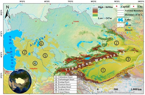
Arid Central Asia (34°21′～55°26′N, 46°28′～96°22′E), located in the heart of Eurasia, includes five former Soviet Union countries (Kazakhstan, Uzbekistan, Turkmenistan, Kyrgyzstan, Tajikistan) and the Xinjiang Uygur autonomous region of China (Figure 1). ACA has a population of more than 100 million and occupies an area of 5668000 km². According to the ESA WorldCover 2020 data, more than 30% of the ACA is covered by deserts (Zanaga et al. 2021). It includes not only famous deserts such as the Taklimakan, Karakum, and the Ustyurt Plateau, but also the dry lakebeds of the Aral Sea, Lake Ebi and Lake Aydin that are caused by human activities and climate change (Ge, Abuduwaili, and Ma 2019). It is also recognized as one of the primary potential SDS sources in the world (Shen et al. 2016). As a priority area for Land Degradation Neutrality (LDN) in the United Nations Sustainable Development Goals (SDGs) 15.3, it is necessary to accurately map SDS sources in ACA (Jiang et al. 2022). Recently, regional climate change has increased wind erosion rates and the frequency of SDS events in ACA (Wang et al. 2020). Evidence from observations (satellite and meteorological stations) and atmospheric model simulations in previous studies indicates a high spatial and temporal variability of SDS activities in this region (Shen et al. 2016; Yuan et al. 2019; Shi et al. 2020).

Figure 1. Geographical location of the study area and spatial distribution of the main deserts in ACA.

3. Materials and methods

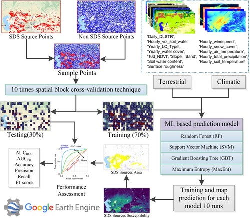
The general process of SDS source prediction and validation is illustrated in Figure 2. The process comprises five main steps, all completed within the GEE platform. First, detected SDS sources and an equal number of non-SDS sources (pseudoabsence points) were combined in this study, and the latter were randomly generated outside a 100-km buffer of the former (Walker et al. 2009). Second, based on the repeated (10 times) spatial block cross-validation (SBCV) technique, 70% of the randomly partitioned spatial blocks was reserved for model training and 30% for validation at each iteration (Crego, Stabach, and Connette 2022). Then, time series of SDS influencing factors (terrestrial and climatic factors) were extracted for each sample date from the multiple data sources accessed by the GEE platform. Next, four ML-based prediction models (RF, GBT, SVM, and MaxEnt model) were built and trained on the training set. An SDS source susceptibility map was then generated as the average probability (0-1) of correct classification across ten model fitting iterations. Pixels with a probability greater than 50% were marked as SDS sources, and a binary SDS source distribution map was generated. Finally, the model performance was assessed based on multiple model evaluation metrics. The accuracy (the training accuracy (TA) and validation accuracy (VA)), precision, recall and F1 score were used to evaluate the model performance. Receiver operator characteristic (ROC) and precision–recall (PR) curves of the different classifiers were also introduced in this study because they can reflect the overall performance of a binary model.

Figure 2. Flowchart of this study in the GEE platform. See Table 1 for detailed land/climate variables.

3.1. SDS source inventory

Accurate SDS source inventory maps are essential for SDS source prediction, especially in arid regions where ground observations are lacking. In this study, an inventory map of SDS sources in Central Asia derived from Moderate Resolution Imaging Spectrometer (MODIS) imagery using the Dust Enhancement Product (DEP) was used. This dataset, which was developed by Nobakht, Shahgedanova, and White (2021), includes the date and location of every SDS outbreak detected between 2003 and 2012. A total of 13642 points were manually detected via visual investigation of DEP images. The upper-left map of Figure 2 shows the spatial distribution of SDS source points. To ensure their validity and reliability, the determined source points of known SDS events were validated against MODIS images. To meet the sample requirements of the classifiers, a negative sample set was randomly generated that deliberately avoids SDS source points.

3.2. SDS source predictor variables

As mentioned above, SDSs are some of the most complex natural hazards regarding dust emission, transport, and coverage (Opp et al. 2021). It is necessary to identify and select effective predictor variables as input datasets for model construction. SDSs are controlled by many factors, including terrestrial and climatic factors. Based on previous research and the characteristics of the study area, 14 SDS source variables, including nine terrestrial factors and five climatic factors, were selected for the classifier training in this study (Gholami, Mohamadifar, et al. 2020b; Nabavi et al. 2018; Rahmati et al. 2020) (Figure 3). The terrestrial factors include the diurnal land surface temperature range (DLSTR), volume of water in the topsoil layer (Vol_Wt_S), land cover type (LCT), water cover (Wt_C), normalized difference vegetation index (NDVI), soil sand content (So_Sa), slope, soil water content (So_Wt), and surface roughness (Sur_R). The climatic factors include the wind speed (Wd_Sp), snow cover (Sn_C), air temperature (A_Temp), total precipitation (T_Prec), and soil temperature (So_Temp).

Figure 3. Thematic maps of SDS source effective predictor variables and RGB image. (a) DLSTR. (b) Vol_Wt_S. (c) LCT. (d) Wt_C. (e) NDVI. (f) So_Sa. (g) Slope. (h) So_Wt. (i) Sur_R. (j) Wd_Sp. (k) Sn_C. (l) A_Temp. (m) T_Prec. (n) So_Temp. (o) RGB image.

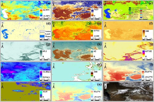
DLSTR can accurately reflect the dry and humid conditions of the land surface (Wang et al. 2021). A daily LST dataset was extracted from the MODIS gap-filled long-term LST dataset retrieved from the awesome-gee-community-datasets (AGCD) repository (Li et al. 2018). Additionally, two soil moisture datasets with varying temporal resolutions retrieved from different datasets were introduced in this study. Vol_Wt_S and So_Wt can reflect instantaneous and long-term soil moisture conditions, respectively (Hersbach et al. 2018; Hengl and Gupta 2019). Due to the emergence and expansion of new SDS sources attributed to human activities in ACA in recent decades, yearly land cover and water body distribution data were also selected (Shen et al. 2016). Considering the high reliability of European Centre for Medium-Range Weather Forecasts (ECMWF) Reanalysis v5 (ERA5) data, the climatic factors in this study were selected during Terra satellite overpass times (Hersbach et al. 2018), thus aligning with the acquisition time of MOD13Q1 data and MODIS true color imagery. Additionally, the values of the input variables differed by several orders of magnitude, which significantly affects the classifier performance. Therefore, to obtain the best overall performance of the ML classifiers, the data were normalized in various ways to reflect the relative significance of the variables (Ahsan et al. 2021). All the datasets used in this study can be accessed from the Earth Engine Data Catalog. Details on the input variables in this study are provided in Table 1.

Table 1. Summary of the input variables in this study.

Category	Variable	Spatial Resolution	Temporal Resolution	Temporal Coverage	Source/Reference
Terrestrial factors	DLSTR	1000 m	daily	2003–2020	AGCD (Li et al. 2018)
	Vol_Wt_S	11132 m	hourly	1982 to present	ERA5 (Hersbach et al. 2018)
	LCT	500 m	yearly	2001 to present	MCD12Q1 (Friedl and Sulla-Menashe 2019)
	Wt_C	30 m	yearly	1984–2021	JRC_GSW (Pekel et al. 2016)
	NDVI	250 m	16-Day	2000 to present	MOD13Q1 (Didan 2021)
	So_Sa	250 m	-	-	OpenLandMap (Hengl 2018)
	Slope	90 m	-	-	SRTM_DEM (Jarvis et al. 2008)
	So_Wt	250 m	-	-	OpenLandMap (Hengl and Gupta 2019)
	Sur_R	90 m	-	-	Geomorpho90 m (Amatulli et al. 2020)
Climatic factors	Wd_Sp	11132 m	hourly	1982 to present	ERA5 (Hersbach et al. 2018)
	Sn_C	11132 m	hourly	1982 to present	ERA5 (Hersbach et al. 2018)
	A_Temp	11132 m	hourly	1982 to present	ERA5 (Hersbach et al. 2018)
	T_Prec	11132 m	hourly	1982 to present	ERA5 (Hersbach et al. 2018)
	So_Temp	11132 m	hourly	1982 to present	ERA5 (Hersbach et al. 2018)

3.3. Machine learning algorithms

Recently, significant progress has been made in ML applications, and models have been proposed for SDS source prediction (Gholami et al. 2021; Rahmati et al. 2020; Boroughani et al. 2022). A total of four efficient ML methods (RF, SVM, GBT, and MaxEnt model) were employed for SDS source prediction. These four models are classical and efficient ML models that are often used for prediction and classification at various spatial and temporal scales, with the (MaxEnt) model as the ML model most commonly adopted in species distribution prediction studies (Yang et al. 2021). Another reason is that this study considers time series samples for model training and requires the use of the GEE platform for analysis, which can provide various models with a consistent performance. Therefore, this study was limited to standard algorithms available on the GEE platform.

Random forest (RF)

The RF model is a nonparametric ensemble learning model that combines the bagging idea and random selection of features typically adopted for regression and classification problems (Teluguntla et al. 2018). As proposed by Breiman (2001), RF is an ensemble classifier comprising many decision trees and outputs the majority vote of individual trees. Each tree is trained through the bootstrap technique referred to as bagging, where the training samples are randomly drawn, with sample repositioning, to generate different subsets. The remaining one-third of the original training sample is employed to create a test set, denotes as the out-of-bag (OOB) samples, which are applied to estimate the training error and calculate the mean decrease accuracy (MDA). In this study, the RF algorithm built into the GEE platform was adopted to calculate the variable importance, referred to as the Gini importance (Strobl et al. 2008). The Gini importance can be calculated as the sum of the Gini impurity decrease across every tree of the forest accumulated every time that a given variable is chosen for node splitting. Here, based on a test-and-trial process, the maximum number of trees was set to 200 in this study. The fraction of input to bag per tree was set to 0.632.

Support vector machine (SVM)

SVM is a supervised learning model involving ML algorithms that can be employed to analyze data for classification and regression analysis (Du et al. 2020). The algorithm searches for a maximum-margin hyperplane able to separate the training data with the most significant possible margin (Boser, Guyon, and Vapnik 1992). The margin is constructed as the space between the decision boundary and the first sample points on each side. Points outside the margin are allowed, while a cost weight is introduced. The cost controlling the trade-off between margin and training errors is particularly important to decrease the impact of outliers. In this study, the cost (C) parameter was set to the default value of 1. The prediction accuracy of the SVM algorithm is affected by the selection of kernel functions such as sigmoid, polynomial, linear, and radial basis functions (RBFs). In this study, the RBF was adopted as the kernel function, which was chosen through test and trial procedures.

Gradient boosting tree (GBT)

GBT, similar to the RF model, is an ensemble learning model that combines decision trees and boosting algorithms (Friedman 2002). The core difference between the RF and GBT models lies in the training process of the decision trees. The decision trees in GBT are sequentially trained, whereas those in RF can be trained in parallel. GBT uses the gradient descent technique as its optimization algorithm to minimize the loss function, which evaluates the performance of decision trees. The other principal difference is the way decisions are output. In regard to RF, the results of all decision trees are aggregated at the end of the training process. GBT, on the other hand, aggregates the results of each decision tree along the way in a fixed order to calculate the final outcome. This is the reason why GBT is sensitive to outliers. Outliers can adversely affect boosting because each tree is built on the residuals or errors of previous trees in this process. In this study, 200 trees and the default loss function, i.e. Least Absolute Deviation, were used.

Maximum entropy (MaxEnt) model

The MaxEnt model was constructed by Phillips, Dudík, and Schapire (2004) and is a niche modeling approach constructed according to the principle of the maximum entropy. The MaxEnt model was initially developed to address the problem of modeling the geographic distribution of a given species. Species distribution modeling (SDM) and SDS source prediction are similar in the sense that both aim to predict geographic regions of interest based on multiple environmental variables (Miller 2010; Hernandez et al. 2006). In the MaxEnt model, the spatial distribution of SDS sources is analogous to the species distribution, and the factors impacting the eco-environmental quality are analogous to SDS source influencing factors (cimatic and terrestrial factors). Additionally, in the language of ML, only a small number of positive samples are available for model training in both cases. Despite its promising potential for SDS source susceptibility assessment, however, the MaxEnt model has not yet been investigated and fully applied. Therefore, the MaxEnt model was introduced as one of the ML methods for SDS source prediction in this study. The MaxEnt model aims to calculate the probability distribution of target occurrences across the set locations. Since the MaxEnt model is a probability mapping algorithm, to evaluate its performance, the continuous probability distribution results of the MaxEnt model were converted into binary results (SDS and non-SDS sources) according to the following rules: the probability distribution is greater than 50% (high and very high SDS source susceptibility levels) for SDS sources and less than 50% (low and medium SDS source susceptibility levels) for non-SDS sources.

3.4. Model evaluation metrics

Ideally, the training and testing samples should be independent in model performance evaluation. For example, validation may be conducted with data retrieved from different geographic regions or spatially distinct subsets of the area over different periods. Thus, the samples were split into training (70%) and testing (30%) subsets (Crego, Stabach, and Connette 2022). The training samples were used for model fitting, and the testing samples were used to evaluate the performance of the trained model. This process can be denoted as the cross-validation (CV) process, and its variants include simple random splits, repeated random splits, or k-fold CV method. Nonetheless, the standard CV methods yield optimistic biased model prediction performance estimates due to spatial autocorrelation (SAC), which is the tendency for the variable values at nearby points to be more similar than those at distant points, especially for SDS source points (Pohjankukka et al. 2017). Therefore, without considering spatial independence between the training and testing samples, the CV results can be overly optimistic estimates of prediction errors and can lead to erroneous scientific conclusions. To solve this problem, the SBCV method was introduced in this study, which is widely used in ecological research (Roberts et al. 2017). First, the study area was divided into spatial blocks of a specified size (a 200-km width was chosen in this study). Then, the 360 spatial blocks were randomly divided into two parts, of which 70% (252) of the blocks was used as training samples and the remaining 30% (108) of the blocks was used as test samples (Figure 2).

In this study, the model performance was also evaluated by measuring the goodness-of-fit and predictive ability of the various ML-based methods. The assessment procedure adopted in this study was based on the binary form of the SDS source susceptibility, in which a confusion matrix was constructed to distinguish between two classes (SDS and non-SDS sources) (Stehman 1997). A true positive (TP) is an outcome where the model correctly predicts the positive class. Similarly, a true negative (TN) is an outcome where the model correctly predicts the negative class. A false positive (FP) is an outcome where the model incorrectly predicts the positive class. A false negative (FN) is an outcome where the model incorrectly predicts the negative class.

Based on the confusion matrix, four performance metrics were calculated, including the accuracy (ACC), positive predictive value (PPV), also referred to as precision, true positive rate (TPR), also referred to as the recall rate or sensitivity, and true negative rate (TNR), also referred to as specificity, which can be calculated as 1 minus the false positive ratio (FPR). Among these metrics, ACC includes TA and VA. The above metrics can be calculated as follows: (1) $Accuracy={\displaystyle \frac{TP+TN}{TP+FN+FP+TN}}$(1) (2) $Precision=PPV={\displaystyle \frac{TP}{TP+FP}}$(2) (3) $Recall=Sensitivity=TPR={\displaystyle \frac{TP}{TP+FN}}$(3) (4) $Specificity=TNR={\displaystyle \frac{TN}{TN+FP}=1-FPR}$(4) (5) $F1score={\displaystyle \frac{2\times PPV\times TPR}{PPV+TPR}}$(5)

Binary classifiers are routinely evaluated with performance measures such as sensitivity (TPR) and specificity (1-FPR), and the performance is frequently visualized with ROC plots (Marzban 2004). The ROC curve is a two-dimensional graph with FPR on the x-axis and TPR on the y-axis. The general performance of the models could be quantitatively evaluated based on the single value of the area under the ROC curve (AUC_ROC). SDSs are sporadic, isolated, and short-lived types of extreme weather events (Liu et al. 2015). The distribution of SDS sources is thus limited, and the number of non-SDS source samples is therefore usually much larger than that of SDS source samples in practice. Although the ROC curve is helpful in performance assessment of a diagnostic test over the range of possible values of a given predictor variable, it can be challenging when the data are heavily imbalanced or when only positive data are of interest. The visual interpretability of ROC plots within the context of imbalanced datasets can be deceptive with respect to conclusions regarding the classification performance reliability (Saito and Rehmsmeier 2015).

The PR curve can provide more information on the model performance than, for instance, the ROC curve when applied to skewed data. Thus, PR curves that evaluate the fraction of TP values among positive predictions can provide the viewer with an accurate prediction of the future classification performance. In this study, another metric was also introduced, namely, the area under the precision–recall curve (AUC_PR), which is more sensitive to improvements in the positive class (SDS source). Similar to the ROC curve, the precision–recall curve is a convex curve that can be plotted using pairs of PPV and TPR values. During the comparison of ML-based classifiers, one classifier is usually considered to outperform another if it achieves a greater area-under-the-curve (AUC) value. The AUC value ranges from 0.5 (baseline performance) to 1 (high performance).

4. Results and discussion

4.1. Model performance evaluation

Based on the SBCV technique, a total of 10 iterations of model fitting and validation were performed for each model. The average performance of the RF, SVM, GBT, and MaxEnt models in SDS source prediction is listed in Table 2. In terms of TA, the performance of the RF, SVM, GBT, and MaxEnt models was estimated at 0.998, 0.886, 0.994, and 0.872, respectively, based on 70% of the sample points used as training data. VA values were also obtained, at approximately 0.875 (RF), 0.860 (SVM), 0.856 (GBT), and 0.859 (MaxEnt), based on 30% of the sample points used as testing data (Table 2). The accuracy values estimated based on both the training and test datasets indicated that RF was the most effective model for SDS source prediction. It was also determined that GBT was susceptible to overfitting during training, whereas the SVM and MaxEnt models were trained well. We also observed a better performance of the RF (0.811) model in terms of precision, followed by that of the GBT (0.793), SVM (0.793) and MaxEnt (0.772) models. Apart from RF (0.889), the MaxEnt model attained the highest average recall rate (0.888). Similarly, the lowest average recall rate (0.862) and F1 score (0.824) were acquired by the SVM model.

Table 2. Performance evaluation of four ML based models.

ML Models	TA	VA	Precision	Recall	F1 Score	AUCROC	AUCPR
RF	0.998	0.875	0.811	0.889	0.847	0.949	0.918
SVM	0.886	0.860	0.793	0.862	0.824	0.920	0.877
GBT	0.994	0.856	0.793	0.866	0.827	0.931	0.887
MaxEnt	0.872	0.859	0.772	0.888	0.825	0.934	0.897

Here, AUC values of the ROC and PR curves were obtained among ten CV iterations on the random subsets of training samples. First, the ROC curve method was used for quantitative validation and comparison of the models. Based on the AUC_ROC results, RF was confirmed as obtaining the best performance (0.949), followed by the MaxEnt (0.934), GBT (0.931), and SVM (0.920) models (Table 2). The AUC_PR results indicated that RF (0.918) was more accurate in SDS source susceptibility prediction than MaxEnt (0.897), GBT (0.887) and SVM (0.877). This finding is consistent with the ML-based landslide susceptibility assessment study of Yang et al. (2022). Similarly, SDS source prediction cannot be regarded as a binary classification problem but as a classification problem for imbalanced datasets (He and Garcia 2009). RF provides advantages over SVM and other classifiers for binary imbalanced classification problems. This finding is consistent with that of He and Garcia (2009), who found that GBDT and RF performed well in resolving samples with a notable class imbalance. To reduce the over- or underestimation degree of the SDS source susceptibility due to the problem of class imbalance, the sampling and model training process was also improved. For example, equal-proportion sampling of SDS and non-SDS sources was used to obtain the training sample set, and ten runs were repeated for model training and prediction.

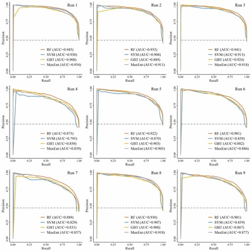
Finally, to compare and assess the stability of the model on random subsets of training samples, ROC and PR curves were generated based on the first nine model iterations. Figure 4 shows the ROC curves of the different ML-based methods in SDS source susceptibility prediction based on nine model iterations. The AUC_ROC value of the four models ranged from 0.888–0.957, indicating that all models attained a satisfactory prediction accuracy in nine iterations, especially the RF model. Figure 5 shows PR curves of the different ML-based methods in SDS source susceptibility prediction. The baseline for the PR curve (dashed line) was determined by the positives (P) and negatives (N). The PR curve results indicated that although the GBT model performed well in terms of the ROC curve, the PR curve results were not stable as expected. This may reduce the reliability of the GBT model in dust source prediction.

Figure 4. ROC curves for the four methods in SDS source susceptibility prediction based on nine model iterations.

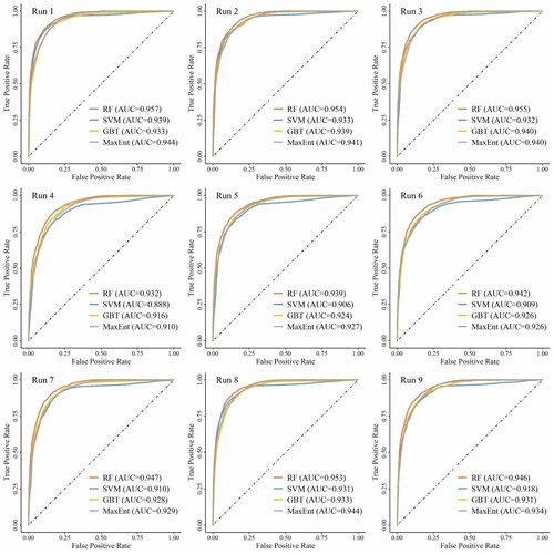
Figure 5. PR curves for the four methods in SDS source susceptibility prediction based on nine model iterations.

Overall, it was demonstrated that the performance of RF was always clearly higher than that of the other models based on both the AUC and other performance evaluation metrics. The obtained results highlight the benefits of tree-based algorithms for complex modeling problems, such as SDS source prediction as a nonlinear phenomenon. In accordance with the obtained results, it has been previously demonstrated that the RF classifier achieves better classification results than SVM when complex multidimensional data such as hyperspectral or multisource data are used (Belgiu and Drăguţ 2016). Despite its high training accuracy, GBT did not perform well in terms of the VA and AUC metrics and was significantly affected by the sample selection process. This suggests that the GBT model could be prone to overfitting in the training process. However, the MaxEnt and SVM models could maintain a suitable balance between their fitting and prediction abilities. Both of these models remained suitably stable and were less affected by the unbalanced distribution of the sample data. Therefore, an in-depth understanding and knowledge of model differences are essential to the application of suitable models at different spatial scales or for a specific research subject. Generally, RF is promising and could be used to map the SDS source susceptibility on larger scales.

4.2. SDS source susceptibility maps

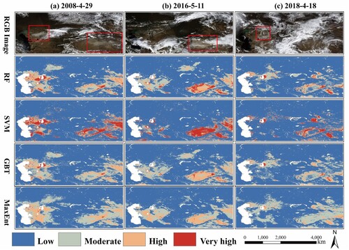
In this study, the susceptibility maps of SDS sources were classified into low (0-0.25), moderate (0.25-0.50), high (0.50-0.75) and very high (0.75-1) susceptibility categories. Nine events (seven SDS events and two non-SDS events) were selected to predict the spatial distribution of SDS sources. These SDS events were selected mainly based on the spatial extent, location and MODIS image quality. The introduction of non-SDS events was mainly employed as a control measure to reveal the prediction model validity and objectivity. MODIS true color images were used to compare and verify the SDS source distributions obtained with the different models. The above nine events were divided into three periods (spring with frequent dust storms, summer and autumn with a satisfactory vegetation cover, and winter with a seasonal snow cover). The purpose of seasonal SDS source susceptibility mapping is to compare the prediction performance between the different models during the different seasons.

The spring season is the most active SDS period in ACA, especially in the Aral Sea (Wang et al. 2022). The dust emissions in spring account for approximately 33%−36% of the annual emissions (Sun, Liu, and Wang 2020). As shown in Figure 6, three SDS events in the Aral Sea region (Aralkum) and Taklimakan Desert were selected. Figure 6(a-b) shows SDSs originating from Aralkum, the Kumtag Desert and the eastern edge of the Taklimakan Desert. Generally, the four ML-based methods could effectively determine the spatial distribution of the SDS source area, but there were variations in the extent of the SDS source susceptibility. The SDS events captured by MODIS are marked in a red box in Figure 6, and these areas should exhibit a higher SDS source susceptibility. The prediction results of the different ML models indicated that RF and SVM were better than GBT and MaxEnt, especially the latter. Although the prediction results based on the MaxEnt model exhibited a wide range for the SDS source susceptibility, the prediction of the very high susceptibility class was nonsignificant. Additionally, the model-predicted SDS source susceptibility varied among the different SDSs, not only in scope but also in scale. The very high SDS source susceptibility rating for the large-scale dust storms that occurred in Aralkum (Figure 6(a)) was higher than that for smaller storms (Figure 6(c)), as was that for the SDS originating in eastern Taklimakan (Figure 6(b)). The study results also suggested that although these areas have not been identified as SDS sources based on satellite images, there is a high potential for the occurrence of SDS sources in these areas, such as the Taklimakan Desert. Since spring is the season with the most severe wind erosion and SDS activity levels in ACA, a wide distribution of SDS sources can generally be considered reasonable under a high wind speed and low vegetation coverage.

Figure 6. SDS source susceptibility maps produced via the ML-based methods in spring. (a) 2008-4-29, (b) 2016-5-11, (c) 2018-4-18.

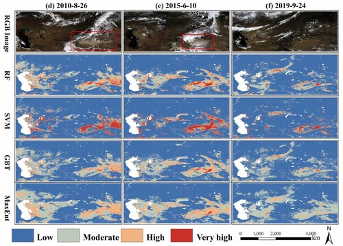
Spatial maps of SDS sources in summer and autumn generated by the four ML-based methods are shown in Figure 7. The MaxEnt model still predicted the broadest range of SDS sources. As an important SDS source in ACA, the SDS source susceptibility prediction performance for eastern Taklimakan was favorable, especially the RF model results (Figure 7). The results revealed that the eastern Taklimakan Desert is the primary SDS source in ACA, which is consistent with the findings of Ge et al. (2014). Although the eastern margin of the Taklimakan is the only low-elevation opening from which low-level dust can flow out of the basin, easterly and northeasterly winds prevail throughout the region almost all year long. Evidence from reanalysis data has indicated that strong northeasterly surface winds associated with low pressures invade the Taklimakan Desert through the eastern corridor and become the main driving force of SDSs in this region (Yumimoto et al. 2009). In addition, a non-SDS event was introduced as a control experiment. As shown in Figure 7(f), although there were no SDS events captured in MODIS imagery, the SVM model results still indicated a high SDS source susceptibility in some areas. Except for the Tianshan Mountains with favorable vegetation conditions, a small part of northern ACA with poor vegetation conditions was predicted as an SDS source (Figure 7(f)).

Figure 7. SDS source susceptibility maps produced using the ML-based methods in summer and autumn. (d) 2010-8-26, (e) 2015-6-10, (f) 2019-9-24.

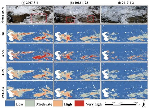
As one of the distinctive features of temperate deserts, snow cover significantly inhibits soil wind erosion in winter (Wang et al. 2020). To assess the performance of the various prediction models under snow cover conditions, three events in winter were selected, two of which were SDS events of different scales (Figure 8(g-h)), and the other was a non-SDS event (Figure 8(i)). Generally, snow cover areas in northern ACA and the Tianshan Mountains exhibit a low SDS source susceptibility. In particular, Figure 8(i) shows that due to snow coverage, the Karakum and Kyzylkum deserts achieve a low SDS source susceptibility, which also indicates that snow cover can reduce the SDS source susceptibility. As shown in Figure 8(g-h), regarding the SDS that occurred in Taklamakan and northern Afghanistan, the SDS source susceptibility was successfully predicted. The loess and alluvial plains of the Amu Darya in northern Afghanistan are important SDS sources in this region (Middleton, Goudie, and Wells 2020). The loose and fine alluvial particles easily lifted by turbulent flow are ideal dust sources (Wen et al. 2019). In total, the model outputs for the nine events described above revealed that reliance on model performance metrics alone is not sufficient and that the spatial distribution of the predicted outcomes is also important for model evaluation. First, the suitable performance of the RF model over the other models in SDS source prediction was demonstrated. For example, SDS sources located in the main deserts could be predicted more clearly with the RF method. Second, the GBT model output results were spatially similarly distributed to the RF results, but the predicted SDS source area with a very high susceptibility was smaller. However, the SVM results indicated a wider distribution of regions with a high SDS source susceptibility. Finally, the SDS source prediction results based on the various ML models exhibited uncertainties in the spatial distribution at the event scale despite the favorable performance in terms of the different evaluation metrics, which could be caused by model overfitting.

Figure 8. SDS source susceptibility maps produced using the ML-based methods in winter. (g) 2007-3-1, (h) 2013-1-23, (i) 2019-1-2.

4.3. Variable contribution analysis

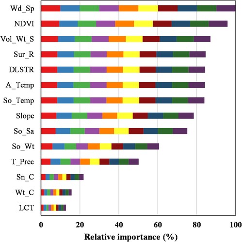
Although arid climate conditions, strong winds, and fragile surface conditions are the most important factors causing SDSs in ACA, determining the contribution of all factors influencing the SDS source distribution is very important to reduce the environmental consequences in this area. In this study, the relative importance of variables controlling the SDS source susceptibility was calculated based on the sum of the decrease in the Gini impurity index over all trees in the RF model (Nembrini, König, and Wright 2018). Therefore, we introduced the relative importance (RI), and the RI value of the most important variable was set to 100%. The RI results for the RF model are shown in Figure 9. The wind speed was determined to yield the greatest contribution to the RF model, followed by NDVI, Vol_Wt_S, Sur_R, So_Temp, A_Temp (LSTDTR), Slope, So_Sa, So_Wt, T_Prec, Sn_C, Wt_C and LC_T. In agreement with our findings, numerous studies have highlighted the significant role of the wind speed in SDS source prediction, especially in arid and semiarid regions (Gholami, Mohammadifar, et al. 2020; Rahmati, Mohammadi, et al. 2020; Ebrahimi-Khusfi et al. 2021). The results further revealed that the vegetation conditions and other land surface characteristics greatly contributed to the SDS source susceptibility prediction performance in our study area. The advantages of native vegetation in soil wind erosion control have also been emphasized in regional studies (Al-Dousari et al. 2020; Xu et al. 2006). Additionally, as expected, land cover, surface water distribution, and snow cover did not contribute as much to the SDS source prediction performance. This may be determined by the spatial and temporal scales in this study. Rahmati, Mohammadi, et al. (2020) and Gholami, Mohammadifar, et al. (2020) highlighted the importance of factors such as land cover in SDS source prediction. However, since this study was conducted at the event scale, the seasonal variation in vegetation may be more important than the annual land cover in SDS source prediction. Likewise, the hourly soil water content factor (Vol_Wt_S) could be more important than the long-term soil characteristic water content factor (So_Wt). Across all of ACA, vegetation conditions play an important role in the current formation and distribution of SDS sources.

Figure 9. Relative importance of the variables to the prediction model outputs based on the random forest.

4.4. Main advantages and Limitations

The main advantages of this study include the application of the GEE platform in SDS event-scale source prediction. Based on the GEE platform, we can directly access the multipetabyte data catalog and the computing resources available to the user. It allows users to incorporate the temporal variability in many predictor datasets, thus providing the opportunity to estimate long-term near-real-time (NRT) SDS source distributions. ML is a powerful technique for Earth observation data analysis. In this study, four classic and efficient ML methods were used for SDS source prediction. Additionally, deep learning and neural network methods supported by TensorFlow or PyTorch can be accessed for training and prediction purposes. The GEE platform is a developing project, and more datasets and new algorithms are constantly being added. We hope that this study will provide resources for a wide range of users, such as governments, researchers, and farmers, who are interested in quickly obtaining NRT high-spatial resolution SDS source maps.

Although we evaluated the predictive performance of four ML methods based on multiple evaluation metrics in this study, the true distribution of SDS sources is crucial for model validation. More information on the spatial distribution of source areas based on SDS events should be used in prediction validation. In the model training process, a large number of non-SDS source points were randomly generated outside a 100-km buffer around SDS source points. With ground and aircraft observations, SDS source points can be associated with individual fields of farmland areas or dry lake beds where the eroding surface area is on the order of 1–100 km² (Walker et al. 2009). Thus, 100 km is the maximum influence range of a given SDS source point, which is defined based on the potential dust source region. However, this can lead to SDS source points being mislabeled as non-SDS source points, which can result in biased predictions. Additionally, while the GEE platform allows users to rapidly analyze large spatial datasets, the higher-resolution data (90 m-Landsat) obtained thus far are difficult to apply to SDS source prediction across ACA. This also restricts the user’s ability to quickly display analysis results in the interactive map interface of GEE. Therefore, we used lower-resolution RS products and reanalysis data in this study. Additionally, upcoming studies should focus on the role of wind speed and vegetation in the control of SDS source areas (Al-Dousari et al. 2020). Relevant thresholds of these variables should also be considered to accurately predict SDS source areas.

5. Conclusion

In this study, combining hourly reanalysis data, RS data and other datasets, we adopted four ML-based methods (RF, SVM, GBT and MaxEnt) to predict SDS sources in ACA at the event scale on the GEE platform. Six metrics (accuracy, precision, recall rate, F1 score, AUC_ROC and AUC_PR) were used to assess the model performance. The results led to the following three main conclusions:

First, these ML-based methods could be employed to successfully predict SDS sources in areas such as Taklimakan, Aralkum, Karakum, the Caspian Sea coast and the middle reaches of the Amu Darya at the event scale. Second, RF performed slightly better than the other ML methods, not only considering its high evaluation metric values but also considering its satisfactory spatial outcome results. In addition, the GBT model was prone to overfitting, and the MaxEnt and SVM models yielded over- and underpredicted SDS source susceptibility results, respectively. Finally, according to the RI value of the variables in SDS source prediction, the wind speed played the most important role in the RF model, followed by vegetation conditions and other land surface characteristics. However, the annual land cover contributed the least to the SDS source prediction performance. The study results demonstrated the feasibility of SDS source region prediction at the event scale based on multisource data and ML models, and the findings could provide a scientific basis for regional land management and planning and serve as a potentially valuable tool for SDS early warning systems.

Acknowledgments

We are grateful to NASA and NOAA for the data support. We thank Google for the GEE, which provided an efficient and powerful computing platform.

Disclosure statement

No potential conflict of interest was reported by the author(s).

Additional information

Funding

This research was partially supported by the National Natural Science Foundation of China (42171014), the UNEP-NSFC International Cooperation Project (42161144004), the Strategic Priority Research Program of the Chinese Academy of Sciences (XDA20060301), National Natural Science Foundation of China (42071424) and the China Scholarship Council (202104910412).

References

- Ahsan, Md M., M. A. Parvez Mahmud, Pritom K. Saha, Kishor D. Gupta, and Zahed Siddique. 2021. “Effect of Data Scaling Methods on Machine Learning Algorithms and Model Performance.” Technologies 9 (3), doi: 10.3390/technologies9030052.
- Al-Dousari, Ali, Ashraf Ramadan, Ayman Al-Qattan, Sara Al-Ateeqi, Hassan Dashti, Modi Ahmed, Noor Al-Dousari, Noof Al-Hashash, and Ahmed Othman. 2020. “Cost and Effect of Native Vegetation Change on Aeolian Sand, Dust, Microclimate and Sustainable Energy in Kuwait.” Journal of Taibah University for Science 14 (1): 628–639. doi: 10.1080/16583655.2020.1761662.
- Amani, M., A. Ghorbanian, S. A. Ahmadi, M. Kakooei, A. Moghimi, S. M. Mirmazloumi, S. H. A. Moghaddam, et al. 2020. “Google Earth Engine Cloud Computing Platform for Remote Sensing Big Data Applications: A Comprehensive Review.” IEEE Journal of Selected Topics in Applied Earth Observations and Remote Sensing 13: 5326–5350. doi: 10.1109/JSTARS.2020.3021052.
- Amatulli, Giuseppe, Daniel McInerney, Tushar Sethi, Peter Strobl, and Sami Domisch. 2020. “Geomorpho90m, Empirical Evaluation and Accuracy Assessment of Global High-Resolution Geomorphometric Layers.” Scientific Data 7 (1): 162. doi: 10.1038/s41597-020-0479-6.
- Belgiu, Mariana, and Lucian Drăguţ. 2016. “Random Forest in Remote Sensing: A Review of Applications and Future Directions.” ISPRS Journal of Photogrammetry and Remote Sensing 114: 24–31. doi: 10.1016/j.isprsjprs.2016.01.011.
- Boroughani, Mahdi, Maziar Mohammadi, Fahimeh Mirchooli, and Stephanie Fiedler. 2022. “Assessment of the Impact of Dust Aerosols on Crop and Water Loss in the Great Salt Desert in Iran.” Computers and Electronics in Agriculture 192: 106605. doi: 10.1016/j.compag.2021.106605.
- Boroughani, Mahdi, Sima Pourhashemi, Hamid Gholami, and Dimitris G. Kaskaoutis. 2021. “Predicting of Dust Storm Source by Combining Remote Sensing, Statistic-Based Predictive Models and Game Theory in the Sistan watershed, southwestern Asia.” Journal of Arid Land 13 (11): 1103–1121. doi: 10.1007/s40333-021-0023-3.
- Boser, Bernhard E., Isabelle M. Guyon, and Vladimir N. Vapnik. 1992. “A Training Algorithm for Optimal Margin Classifiers.” In Proceedings of the fifth annual workshop on Computational learning theory, 144–52. Pittsburgh, Pennsylvania, USA: Association for Computing Machinery.
- Breiman, Leo. 2001. “Random Forests.” Machine Learning 45 (1): 5–32. doi: 10.1023/A:1010933404324.
- Butt, Mohsin Jamil, Mazen Ebraheem Assiri, and Essam Mohammed Alghamdi. 2023. “A New Approach for Sand and Dust Storm Monitoring Using Satellite Data.” In Mediterranean Geosciences Union Annual Meeting. Marrakech, Morocco.
- Butt, Mohsin Jamil, and AbdulWahab S. Mashat. 2018. “MODIS Satellite Data Evaluation for Sand and Dust Storm Monitoring in Saudi Arabia.” International Journal of Remote Sensing 39 (23): 8627–8645. doi: 10.1080/01431161.2018.1488293.
- Crego, Ramiro D., Jared A. Stabach, and Grant Connette. 2022. “Implementation of Species Distribution Models in Google Earth Engine.” Diversity and Distributions 28 (5): 904–916. doi: 10.1111/ddi.13491.
- Darmenova, Kremena, Irina N. Sokolik, Yaping Shao, Beatrice Marticorena, and Gilles Bergametti. 2009. “Development of a Physically Based Dust Emission Module Within the Weather Research and Forecasting (WRF) model: Assessment of Dust Emission Parameterizations and Input Parameters for Source Regions in Central and East Asia.” Journal of Geophysical Research: Atmospheres 114: D14. doi: 10.1029/2008JD011236.
- Darvishi Boloorani, Ali, Najmeh Neysani Samany, Ramin Papi, and Masoud Soleimani. 2022. “Dust Source Susceptibility Mapping in Tigris and Euphrates Basin Using Remotely Sensed Imagery.” CATENA 209: 105795. doi: 10.1016/j.catena.2021.105795.
- Dehshiri, Hosseini, Seyyed Shahabaddin, Bahar Firoozabadi, and Hossein Afshin. 2022. “A New Application of Multi-Criteria Decision Making in Identifying Critical Dust Sources and Comparing Three Common Receptor-Based Models.” Science of The Total Environment 808: 152109. doi: 10.1016/j.scitotenv.2021.152109.
- Didan, K. 2021. “MODIS/Terra Vegetation Indices 16-Day L3 Global 250 m SIN Grid V061.” In.: NASA EOSDIS Land Processes DAAC.
- Doronzo, Domenico M., Ali Al-Dousari, Arnau Folch, and Pavla Dagsson-Waldhauserova. 2016. “Preface to the Dust Topical Collection.” Arabian Journal of Geosciences 9 (6): 468. doi: 10.1007/s12517-016-2504-9.
- Du, Peijun, Xuyu Bai, Kun Tan, Zhaohui Xue, Alim Samat, Junshi Xia, Erzhu Li, Hongjun Su, and Wei Liu. 2020. “Advances of Four Machine Learning Methods for Spatial Data Handling: a Review.” Journal of Geovisualization and Spatial Analysis 4 (1): 13. doi: 10.1007/s41651-020-00048-5.
- Ebrahimi-Khusfi, Zohre, Ruhollah Taghizadeh-Mehrjardi, Fatemeh Roustaei, Mohsen Ebrahimi-Khusfi, Amir Hosein Mosavi, Brandon Heung, Mojtaba Soleimani-Sardo, and Thomas Scholten. 2021. “Determining the Contribution of Environmental Factors in Controlling Dust Pollution During Cold and Warm Months of Western Iran Using Different Data Mining Algorithms and Game Theory.” Ecological Indicators 132: 108287. doi: 10.1016/j.ecolind.2021.108287.
- Friedl, M., and D. Sulla-Menashe. 2019. “MCD12Q1 MODIS/Terra+Aqua Land Cover Type Yearly L3 Global 500 m SIN Grid V006.” In.: NASA EOSDIS Land Processes DAAC.
- Friedman, Jerome H. 2002. “Stochastic Gradient Boosting.” Computational Statistics & Data Analysis 38 (4): 367–378. doi: 10.1016/S0167-9473(01)00065-2.
- Ge, Yongxiao, Jilili Abuduwaili, and Long Ma. 2019. “Lakes in Arid Land and Saline Dust Storms.” E3S Web Conf. 99: 01007. doi: 10.1051/e3sconf/20199901007.
- Ge, J. M., J. P. Huang, C. P. Xu, Y. L. Qi, and H. Y. Liu. 2014. “Characteristics of Taklimakan Dust Emission and Distribution: A Satellite and Reanalysis Field Perspective.” Journal of Geophysical Research: Atmospheres 119 (20): 11,772–111,83. doi: 10.1002/2014JD022280.
- Gholami, Hamid, Aliakbar Mohamadifar, Armin Sorooshian, and John D. Jansen. 2020a. “Machine-Learning Algorithms for Predicting Land Susceptibility to Dust Emissions: The Case of the Jazmurian Basin, Iran.” Atmospheric Pollution Research 11 (8): 1303–1315. doi: 10.1016/j.apr.2020.05.009.
- Gholami, Hamid, Aliakbar Mohammadifar, Hossein Malakooti, Yahya Esmaeilpour, Shahram Golzari, Fariborz Mohammadi, Yue Li, et al. 2021. “Integrated Modelling for Mapping Spatial Sources of Dust in Central Asia - An Important Dust Source in the Global Atmospheric System.” Atmospheric Pollution Research 12 (9): 101173. doi: 10.1016/j.apr.2021.101173.
- Gholami, Hamid, Aliakbar Mohammadifar, Hamid Reza Pourghasemi, and Adrian L. Collins. 2020b. “A New Integrated Data Mining Model to Map Spatial Variation in the Susceptibility of Land to Act as a Source of Aeolian Dust.” Environmental Science and Pollution Research 27 (33): 42022–42039. doi: 10.1007/s11356-020-10168-6.
- Gorelick, Noel, Matt Hancher, Mike Dixon, Simon Ilyushchenko, David Thau, and Rebecca Moore. 2017. “Google Earth Engine: Planetary-Scale Geospatial Analysis for Everyone.” Remote Sensing of Environment 202: 18–27. doi: 10.1016/j.rse.2017.06.031.
- Guo, Huadong, Zhen Liu, Hao Jiang, Changlin Wang, Jie Liu, and Dong Liang. 2017. “Big Earth Data: A New Challenge and Opportunity for Digital Earth’s Development.” International Journal of Digital Earth 10 (1): 1–12. doi: 10.1080/17538947.2016.1264490.
- Hancher, M. 2017. “New Techniques for Deep Learning with Geospatial Data using TensorFlow, Earth Engine, and Google Cloud Platform.” In, IN11E-08.
- Hansen, M. C., P. V. Potapov, R. Moore, M. Hancher, S. A. Turubanova, A. Tyukavina, D. Thau, et al. 2013. “High-Resolution Global Maps of 21st-Century Forest Cover Change.” Science 342 (6160): 850–853. doi: 10.1126/science.1244693.
- He, H., and E. A. Garcia. 2009. “Learning from Imbalanced Data.” IEEE Transactions on Knowledge and Data Engineering 21 (9): 1263–1284. doi: 10.1109/TKDE.2008.239.
- Hengl, Tomislav. 2018. “Sand content in % (kg / kg) at 6 standard depths (0, 10, 30, 60, 100 and 200 cm) at 250 m resolution (Version v02).” In.: Zenodo.
- Hengl, Tomislav, and Surya Gupta. 2019. “Soil Water Content (volumetric %) for 33kPa and 1500kPa Suctions Predicted at 6 Standard Depths (0, 10, 30, 60, 100 and 200 cm) at 250 m resolution (Version v01).” In.: Zenodo.
- Hernandez, Pilar A., Catherine H. Graham, Lawrence L. Master, and Deborah L. Albert. 2006. “The Effect of Sample Size and Species Characteristics on Performance of Different Species Distribution Modeling Methods.” Ecography 29 (5): 773–785. doi: 10.1111/j.0906-7590.2006.04700.x.
- Hersbach, H., B. Bell, P. Berrisford, G. Biavati, A. Horányi, J. Muñoz Sabater, J. Nicolas, C. Peubey, R. Radu, and I. Rozum. 2018. “ERA5 hourly data on single levels from 1979 to present.” In, edited by Copernicus Climate Change Service (C3S) Climate Data Store (CDS).
- Holloway, Jacinta, and Kerrie Mengersen. 2018. “Statistical Machine Learning Methods and Remote Sensing for Sustainable Development Goals: A Review.” Remote Sensing 10 (9), doi: 10.3390/rs10091365.
- Huang, Qunying, Chaowei Yang, Karl Benedict, Songqing Chen, Abdelmounaam Rezgui, and Jibo Xie. 2013. “Utilize Cloud Computing to Support Dust Storm Forecasting.” International Journal of Digital Earth 6 (4): 338–355. doi: 10.1080/17538947.2012.749949.
- Jarvis, Andy, Hannes Isaak Reuter, Andrew Nelson, and Edward Guevara. 2008. “Hole-filled SRTM for the globe Version 4.” In.: CGIAR-CSI SRTM 90 m Database.
- Jiang, Liangliang, Anming Bao, Guli Jiapaer, Rui Liu, Ye Yuan, and Tao Yu. 2022. “Monitoring Land Degradation and Assessing Its Drivers to Support Sustainable Development Goal 15.3 in Central Asia.” Science of The Total Environment 807: 150868. doi: 10.1016/j.scitotenv.2021.150868.
- Jiao, Pengcheng, Jiajun Wang, Xinwei Chen, Jiani Ruan, Xinghong Ye, and Amir H. Alavi. 2021. “Next-Generation Remote Sensing and PREDICTION of Sand and Dust Storms: State-of-the-Art and Future Trends.” International Journal of Remote Sensing 42 (14): 5277–5316. doi: 10.1080/01431161.2021.1912433.
- Jilili, Abuduwaili, Dong Wei Liu, and Guang Yang Wu. 2010. “Saline Dust Storms and Their Ecological Impacts in Arid Regions.” Journal of Arid Land 2 (2): 144–150. doi: 10.3724/sp.J.1227.2010.00144.
- Kennedy, Robert E., Zhiqiang Yang, Noel Gorelick, Justin Braaten, Lucas Cavalcante, Warren B. Cohen, and Sean Healey. 2018. “Implementation of the LandTrendr Algorithm on Google Earth Engine.” Remote Sensing 10 (5), doi: 10.3390/rs10050691.
- Knippertz, Peter, and Martin C. Todd. 2012. “Mineral dust aerosols over the Sahara: Meteorological controls on emission and transport and implications for modeling.” Reviews of Geophysics 50 (1), doi: 10.1029/2011RG000362.
- Kong, Dongdong, Yongqiang Zhang, Xihui Gu, and Dagang Wang. 2019. “A Robust Method for Reconstructing Global MODIS EVI Time Series on the Google Earth Engine.” ISPRS Journal of Photogrammetry and Remote Sensing 155: 13–24. doi: 10.1016/j.isprsjprs.2019.06.014.
- Labban, Abdulhaleem H., and Mohsin Jamil Butt. 2021. “Analysis of Sand and Dust Storm Events Over Saudi Arabia in Relation with Meteorological Parameters and ENSO.” Arabian Journal of Geosciences 14 (1): 22. doi: 10.1007/s12517-020-06291-w.
- Lary, David J., Amir H. Alavi, Amir H. Gandomi, and Annette L. Walker. 2016. “Machine Learning in Geosciences and Remote Sensing.” Geoscience Frontiers 7 (1): 3–10. doi: 10.1016/j.gsf.2015.07.003.
- Li, Xiaoma, Yuyu Zhou, Ghassem R. Asrar, and Zhengyuan Zhu. 2018. “Creating a Seamless 1 km Resolution Daily Land Surface Temperature Dataset for Urban and Surrounding Areas in the Conterminous United States.” Remote Sensing of Environment 206: 84–97. doi: 10.1016/j.rse.2017.12.010.
- Liakos, Konstantinos G., Patrizia Busato, Dimitrios Moshou, Simon Pearson, and Dionysis Bochtis. 2018. “Machine Learning in Agriculture: A Review.” Sensors 18 (8), doi: 10.3390/s18082674.
- Liu, Xueqin, Ning Li, Shuai Yuan, Ning Xu, Wenqin Shi, and Weibin Chen. 2015. “The Joint Return Period Analysis of Natural Disasters Based on Monitoring and Statistical Modeling of Multidimensional Hazard Factors.” Science of The Total Environment 538: 724–732. doi: 10.1016/j.scitotenv.2015.08.093.
- Marzban, Caren. 2004. “The ROC Curve and the Area under It as Performance Measures.” Weather and Forecasting 19 (6): 1106–1114. doi: 10.1175/825.1.
- Middleton, Nicholas John, Andrew S Goudie, and Gordon L Wells. 2020. “The frequency and source areas of dust storms.” In Aeolian geomorphology, 237–259. Routledge.
- Miller, Jennifer. 2010. “Species Distribution Modeling.” Geography Compass 4 (6): 490–509. doi: 10.1111/j.1749-8198.2010.00351.x.
- Nabavi, Seyed Omid, Leopold Haimberger, Reyhaneh Abbasi, and Cyrus Samimi. 2018. “Prediction of Aerosol Optical Depth in West Asia Using Deterministic Models and Machine Learning Algorithms.” Aeolian Research 35: 69–84. doi: 10.1016/j.aeolia.2018.10.002.
- Nembrini, Stefano, Inke R. König, and Marvin N. Wright. 2018. “The Revival of the Gini Importance?” Bioinformatics (oxford, England) 34 (21): 3711–3718. doi: 10.1093/bioinformatics/bty373.
- Nobakht, Mohamad, Maria Shahgedanova, and Kevin White. 2021. “New Inventory of Dust Emission Sources in Central Asia and Northwestern China Derived From MODIS Imagery Using Dust Enhancement Technique.” Journal of Geophysical Research: Atmospheres 126 (4): e2020JD033382. doi: 10.1029/2020JD033382.
- Opp, Christian, Michael Groll, Hamidreza Abbasi, and Mansour A. Foroushani. 2021. “Causes and Effects of Sand and Dust Storms: What Has Past Research Taught Us? A Survey.” Journal of Risk and Financial Management 14 (7), doi: 10.3390/jrfm14070326.
- Papi, Ramin, A. A. Kakroodi, Masoud Soleimani, Leyla Karami, Fatemeh Amiri, and Seyed Kazem Alavipanah. 2022. “Identifying Sand and Dust Storm Sources Using Spatial-Temporal Analysis of Remote Sensing Data in Central Iran.” Ecological Informatics 70: 101724. doi: 10.1016/j.ecoinf.2022.101724.
- Pekel, Jean-François, Andrew Cottam, Noel Gorelick, and Alan S. Belward. 2016. “High-Resolution Mapping of Global Surface Water and Its Long-Term Changes.” Nature 540 (7633): 418–422. doi: 10.1038/nature20584.
- Phillips, Steven J., Miroslav Dudík, and Robert E. Schapire. 2004. “A Maximum Entropy Approach to Species Distribution Modeling.” In Proceedings of the twenty-first international conference on Machine learning, 83. Banff, Alberta, Canada: Association for Computing Machinery.
- Pohjankukka, Jonne, Tapio Pahikkala, Paavo Nevalainen, and Jukka Heikkonen. 2017. “Estimating the Prediction Performance of Spatial Models Via Spatial K-Fold Cross Validation.” International Journal of Geographical Information Science 31 (10): 2001–2019. doi: 10.1080/13658816.2017.1346255.
- Rahmati, Omid, Farnoush Mohammadi, Seid Saeid Ghiasi, John Tiefenbacher, Davoud Davoudi Moghaddam, Frederic Coulon, Omid Asadi Nalivan, and Dieu Tien Bui. 2020a. “Identifying Sources of Dust Aerosol Using a New Framework Based on Remote Sensing and Modelling.” Science of The Total Environment 737: 139508. doi: 10.1016/j.scitotenv.2020.139508.
- Rahmati, Omid, Mahdi Panahi, Seid Saeid Ghiasi, Ravinesh C. Deo, John P. Tiefenbacher, Biswajeet Pradhan, Ali Jahani, et al. 2020b. “Hybridized Neural Fuzzy Ensembles for Dust Source Modeling and Prediction.” Atmospheric Environment 224: 117320. doi: 10.1016/j.atmosenv.2020.117320.
- Rayegani, Behzad, Susan Barati, Hamid Goshtasb, Saba Gachpaz, Javad Ramezani, and Hamid Sarkheil. 2020. “Sand and Dust Storm Sources Identification: A Remote Sensing Approach.” Ecological Indicators 112: 106099. doi: 10.1016/j.ecolind.2020.106099.
- Roberts, David R., Volker Bahn, Simone Ciuti, Mark S. Boyce, Jane Elith, Gurutzeta Guillera-Arroita, Severin Hauenstein, et al. 2017. “Cross-Validation Strategies for Data with Temporal, Spatial, Hierarchical, or Phylogenetic Structure.” Ecography 40 (8): 913–929. doi: 10.1111/ecog.02881.
- Saito, Takaya, and Marc Rehmsmeier. 2015. “The Precision-Recall Plot Is More Informative than the ROC Plot When Evaluating Binary Classifiers on Imbalanced Datasets.” PLOS ONE 10 (3): e0118432. doi: 10.1371/journal.pone.0118432.
- Schepanski, Kerstin. 2018. “Transport of Mineral Dust and Its Impact on Climate.” Geosciences 8 (5), doi: 10.3390/geosciences8050151.
- Shen, Hao, Jilili Abuduwaili, Alim Samat, and Long Ma. 2016. “A Review on the Research of Modern Aeolian Dust in Central Asia.” Arabian Journal of Geosciences 9 (13): 625. doi: 10.1007/s12517-016-2646-9.
- Shi, Lamei, Jiahua Zhang, Da Zhang Fengmei Yao, and Huadong Guo. 2020. “Temporal Variation of Dust Emissions in Dust Sources Over Central Asia in Recent Decades and the Climate Linkages.” Atmospheric Environment 222: 117176. doi: 10.1016/j.atmosenv.2019.117176.
- Stehman, Stephen V. 1997. “Selecting and Interpreting Measures of Thematic Classification Accuracy.” Remote Sensing of Environment 62 (1): 77–89. doi: 10.1016/S0034-4257(97)00083-7.
- Strobl, Carolin, Anne-Laure Boulesteix, Thomas Kneib, Thomas Augustin, and Achim Zeileis. 2008. “Conditional Variable Importance for Random Forests.” BMC Bioinformatics 9 (1): 307. doi: 10.1186/1471-2105-9-307.
- Sun, Hui, Xiaodong Liu, and Anqi Wang. 2020. “Seasonal and Interannual Variations of Atmospheric Dust Aerosols in Mid and Low Latitudes of Asia – A Comparative Study.” Atmospheric Research 244: 105036. doi: 10.1016/j.atmosres.2020.105036.
- Tamiminia, Haifa, Bahram Salehi, Masoud Mahdianpari, Lindi Quackenbush, Sarina Adeli, and Brian Brisco. 2020. “Google Earth Engine for Geo-Big Data Applications: A Meta-Analysis and Systematic Review.” ISPRS Journal of Photogrammetry and Remote Sensing 164: 152–170. doi: 10.1016/j.isprsjprs.2020.04.001.
- Teluguntla, Pardhasaradhi, Prasad S. Thenkabail, Adam Oliphant, Jun Xiong, Murali Krishna Gumma, Russell G. Congalton, Kamini Yadav, and Alfredo Huete. 2018. “A 30-m Landsat-Derived Cropland Extent Product of Australia and China Using Random Forest Machine Learning Algorithm on Google Earth Engine Cloud Computing Platform.” ISPRS Journal of Photogrammetry and Remote Sensing 144: 325–340. doi: 10.1016/j.isprsjprs.2018.07.017.
- Walker, Annette L., Ming Liu, Steven D. Miller, Kim A. Richardson, and Douglas L. Westphal. 2009. “Development of a Dust Source Database for Mesoscale Forecasting in Southwest Asia.” Journal of Geophysical Research: Atmospheres 114 (D18), doi: 10.1029/2008JD011541.
- Wang, Wei, Alim Samat, Jilili Abuduwaili, and Yongxiao Ge. 2021. “Quantifying the influences of land surface parameters on LST variations based on GeoDetector model in Syr Darya Basin, Central Asia.” Journal of Arid Environments 186: 104415. doi: 10.1016/j.jaridenv.2020.104415.
- Wang, Wei, Alim Samat, Jilili Abuduwaili, Yongxiao Ge, Philippe De Maeyer, and Tim Van de Voorde. 2022. “Temporal Characterization of Sand and Dust Storm Activity and Its Climatic and Terrestrial Drivers in the Aral Sea region.” Atmospheric Research 275: 106242. doi: 10.1016/j.atmosres.2022.106242.
- Wang, Wei, Alim Samat, Yongxiao Ge, Long Ma, Abula Tuheti, Shan Zou, and Jilili Abuduwaili. 2020. “Quantitative Soil Wind Erosion Potential Mapping for Central Asia Using the Google Earth Engine Platform.” Remote Sensing 12 (20), doi: 10.3390/rs12203430.
- Wen, Yanglei, Yongqiu Wu, Lihua Tan, Dawei Li, and Tianyang Fu. 2019. “End-Member Modeling of the Grain Size Record of Loess in the Mu Us Desert and Implications for Dust Sources.” Quaternary International 532: 87–97. doi: 10.1016/j.quaint.2019.10.005.
- Wu, Yao, Bo Wen, Shanshan Li, and Yuming Guo. 2021. “Sand and dust storms in Asia: a call for global cooperation on climate change.” The Lancet Planetary Health 5 (6): e329–ee30. doi: 10.1016/S2542-5196(21)00082-6.
- Xu, Xingkui, Jason K. Levy, Lin Zhaohui, and Chen Hong. 2006. “An Investigation of Sand–Dust Storm Events and Land Surface Characteristics in China Using NOAA NDVI Data.” Global and Planetary Change 52 (1): 182–196. doi: 10.1016/j.gloplacha.2006.02.009.
- Yang, Zongbao, Yang Bai, Juha M. Alatalo, Zhongde Huang, Fen Yang, Xiaoyan Pu, Ruibo Wang, Wei Yang, and Xueyan Guo. 2021. “Spatio-Temporal Variation in Potential Habitats for Rare and Endangered Plants and Habitat Conservation Based on the Maximum Entropy Model.” Science of The Total Environment 784: 147080. doi: 10.1016/j.scitotenv.2021.147080.
- Yang, Can, Lei-Lei Liu, Faming Huang, Lei Huang, and Xiao-Mi Wang. 2022. “Machine Learning-Based Landslide Susceptibility Assessment with Optimized Ratio of Landslide to Non-Landslide Samples.” Gondwana Research, doi: 10.1016/j.gr.2022.05.012.
- Youlin, Yang, Victor Squires, and Lu Qi. 2002. Global alarm: dust and sandstorms from the world's drylands. Beijing: United Nations Convention to Combat Desertification (UNCCD).
- Yu, Manzhu, Myra Bambacus, Guido Cervone, Keith Clarke, Daniel Duffy, Qunying Huang, Jing Li, et al. 2020. “Spatiotemporal Event Detection: A Review.” International Journal of Digital Earth 13 (12): 1339–1365. doi: 10.1080/17538947.2020.1738569.
- Yuan, Tiangang, Siyu Chen, Jianping Huang, Xiaorui Zhang, Yuan Luo, Xiaojun Ma, and Guolong Zhang. 2019. “Sensitivity of Simulating a Dust Storm Over Central Asia to Different Dust Schemes Using the WRF-Chem Model.” Atmospheric Environment 207: 16–29. doi: 10.1016/j.atmosenv.2019.03.014.
- Yumimoto, K., K. Eguchi, I. Uno, T. Takemura, Z. Liu, A. Shimizu, and N. Sugimoto. 2009. “An Elevated Large-Scale Dust Veil from the Taklimakan Desert: Intercontinental Transport and Three-Dimensional Structure as Captured by CALIPSO and Regional and Global Models.” Atmospheric Chemistry and Physics 9 (21): 8545–8558. doi: 10.5194/acp-9-8545-2009.
- Zanaga, D., R. Van De Kerchove, W. De Keersmaecker, N. Souverijns, C. Brockmann, R. Quast, J. Wevers, A. Grosu, A. Paccini, and S. Vergnaud. 2021. “ESA WorldCover 10 m 2020 v100.” In, edited by ESA. Zenodo.