A new denoising method for photon-counting LiDAR data with different surface types and observation conditions

ABSTRACT

Spaceborne photon-counting LiDAR is significantly affected by noise, and existing denoising algorithms cannot be universally adapted to different surface types and topographies under all observation conditions. Accordingly, a new denoising method is presented to extract signal photons adaptively. The method includes two steps. First, the local neighborhood radius is calculated according to photons' density, then the first-step denoising process is completed via photons’ curvature feature based on KNN search and covariance matrix. Second, the local photon filtering direction and threshold are obtained based on the first-step denoising results by RANSAC and elevation frequency histogram, and the local dense noise photons that the first-step cannot be identified are further eliminated. The following results are drawn: (1) experimental results on MATLAS with different topographies indicate that the average accuracy of second-step denoising exceeds 0.94, and the accuracy is effectively improves with the number of denoising times; (2) experiments on ICESat-2 under different observation conditions demonstrate that the algorithm can accurately identify signal photons in different surface types and topographies. Overall, the proposed algorithm has good adaptability and robustness for adaptive denoising of large-scale photons, and the denoising results can provide more reasonable and reliable data for sustainable urban development.

KEYWORDS:

• Photon-counting LiDAR
• adaptive denoising
• complex surface types and topographies
• MATLAS
• ICESat-2

1. Introduction

Spaceborne LiDAR has the advantage of fast and direct access to high-precision three-dimensional (3D) information on the Earth's surface and global geographic coverage. This technology provides dynamic and periodic rich information to realize sustainable development goals, especially for those closely related to the environment and resources on the Earth's surface (Zhang et al. 2022; Zhu et al. 2022). These goals can be realized by integrating and analysing data on the land, ocean, and human activities to comprehensively understand a vast region (Chen, Xu, and Gong 2021; Chen et al. 2022; Guo et al. 2021). The Geoscience Laser Altimeter System (GLAS) instrument on the Ice, Cloud, and land Elevation Satellite-1(ICESat-1) has provided various scientific data for sustainable development goals including sea ice thickness change, urban building height, and forest vertical structure parameters (Gong et al. 2011; Xing et al. 2010; Zwally et al. 2002). As a follow-up mission to ICESat-1, ICESat-2 was successfully launched in September 2018. The Advanced Topographic Laser Altimeter System (ATLAS) onboard ICESat-2 employs six laser beams divided into three pairs (each pair consists of a strong and a weak beam with an energy ratio of about 4:1) with micro-pulse photon-counting technology (Markus et al. 2017; Yu et al. 2021). This results in a higher sensitivity, higher repetition rate (10KHz), and lower energy than GLAS, and provides photons of different surface types along the track with smaller footprints (diameter of ∼ 11 m) and higher density (approximately 0.7 m interval along-track) (Mulverhill et al. 2022; Neumann et al. 2019). This is the application of this technology to spaceborne platforms worldwide, and represents an important future trend for laser altimeters. However, due to the low energy of the transmitted laser (several tens of μJ), the returned signal photons are susceptible to solar radiation, atmospheric scattering, instrument, and post-pulsing noise photons when detecting useful information, making the accurate extraction of effective signals challenging. This influence is especially apparent during the daytime. The number of signal photons is usually less that of noise photons, making it difficult to recognize signal photons due to the low signal-to-noise ratio (SNR) (Ma et al. 2018; Neuenschwander and Pitts 2019). Therefore, the noise removal is necessary for the data pre-processing and application of photon-counting LiDAR.

Given that signal photons are more densely distributed in the space than noise photons, scholars at home and abroad have designed and implemented a range of supervised and unsupervised classification algorithms. The idea of supervised classification is to separate signal and noise photons by constructing photon data features and combining related supervised classification algorithms (Chen et al. 2019; Zang, Lin, and Liang 2017). There are two categories of unsupervised classification algorithms: rasterizing the photon data into a two-dimensional (2D) image, then employing image processing methods such as edge and region detection to identify noise (Magruder et al. 2012). However, the former loses point cloud information, whereas the latter is based on 2D profile photons using local statistical parameters (e.g. photon elevation, density, distance, and eigenvector and its distribution characteristics). Single-level or multi-level filters have been utilized to extract signal photons, such as window statistics (Gwenzi et al. 2016; Neumann et al. 2021; Popescu et al. 2018), density clustering with different filter kernel shapes (Wang et al. 2021; Zhang and Kerekes 2015; Zhang, Zhou, and Luo 2022; Zhu et al. 2021), single-parameter or multi-parameter combination (Herzfeld et al. 2017; Nie et al. 2018; Xia et al. 2014), three-dimensional voxel method (Tang et al. 2016), and point cloud distribution center expressed by radial basis functions (Herzfeld et al. 2014).

Generally speaking, the above methods can provide good performance for strong or weak beam data with a specific surface type, such as vegetation, residential areas, water bodies, plains, and mountains. However, in practice, processing the whole data usually has to deal with various surface types. The terrain characteristics and reflectivity are different for diverse surface types, and the density of the noise photons is also quite different. Significantly, signal photons from weak beam data are just as important as those from strong beam data. If the signal photons in the strong and weak beam data cannot be accurately identified simultaneously, half of the data is idle. Therefore, the adaptability and reliability of the proposed algorithm needs further verification. Aiming at the denoising demand for data with various surface types under different observation conditions, this paper supplements additional geometric features such as curvature and direction apart from the traditional statistical parameters such as density and elevation, to better reflect the morphological characteristics of point cloud clusters for realizing automatic and refined photon denoising processing.

2. Dataset and methods

2.1 Dataset

2.1.1 ICESat-2/ATLAS data

ICESat-2/ATLAS data are freely provided by the official website of the National Snow and Ice Data Center (NSIDC) (https://nsidc.org/data/icesat-2/data-sets). It contains 21 geophysical products arranged in four levels, namely ATL00 – ATL021 (Markus et al. 2017). In this paper, the ATL03 global positioning photon data are selected to perform the experiment, where each data records the precise longitude, latitude, elevation, time, and other parameter information of all photons. The topographical features and observation conditions primarily determine the differences in density and SNR of ATLAS photon data (Nie et al. 2018). Based on the above principles, relevant experimental data are selected in this study to verify the algorithm’s robustness and universality. The data information is shown in Table 1 and Figure 1.

Figure 1. The distribution of raw ATLAS data. (a) Data A_gt1 l, (b) Data A_gt1r, (c) Data B_gt1 l, (d) Data B_gt1r.

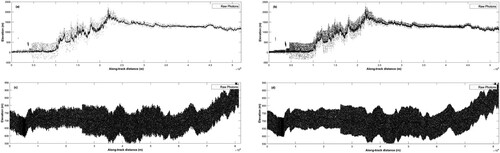
Table 1. Data information of ATLAS.

Series	Time	Dataset	Length	Region	Track	Number
Data A	Nighttime	ATL03_20191013141552_02550502	520km	115.72∼116.32 39.35∼44.05	gt1l	353,180
					gt1r	1,441,090
Data B	Daytime	ATL03_20200412053524_02550702	82km	114.81∼114.92 49.26∼49.98	gt1l	280,944
					gt1r	467,806

2.1.2 MATLAS data

Since there are no quantitative reference results to evaluate the denoising effect of ATLAS data, this paper employs the MATLAS simulation data, which has the official classification results between signal and noise provided by NASA, to evaluate the algorithm’s performance (https://icesat-2.gsfc.nasa.gov/legacy-data/matlas/matlas_data. php). The MATLAS data are generated from the airborne MABEL data by adjusting detected number of photons regarding the parameter configuration of the ATLAS instrument. As the most approximate dataset to the actual situation of the satellite, it can be obtained from the official portal (Chen et al. 2019). Table 2 shows the data information of MATLAS, including six datasets covering different terrain and coverage areas in Virginia, West Coast, and East Coast of the United States. The SNR in Table 2 is calculated according to official classification results provided by NASA.

Table 2. Data information of MATLAS.

Site	Terrain	Canopy Closure Fraction	Data name	Beam	Photon number	SNR
East Coast	Gentle hill	90%	t231600_010_2_8B_1VEG	Strong	45,225	0.79
				Weak	30,448	0.20
			t231600_010_2_8B_2VEG	Strong	21,969	10.79
				Weak	6,938	2.72
Virginia	Flat terrain	55%	t222500_010_2_8a_2VEG	Strong	54,686	1.09
				Weak	33,276	0.27
			t222500_010_2_8a_3VEG	Strong	30,440	15.44
				Weak	9,132	3.93
West Coast	Mountain	90%	t024900_010_2_8C_1VEG	Strong	42,632	0.79
				Weak	28,739	0.20
			t024900_010_2_8C_2VEG	Strong	20,709	11.13
				Weak	6,416	2.76

2.2 Methods

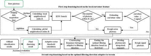
The proposed algorithm framework includes the first-step denoising based on the local curvature features, the second-step denoising based on main direction and adaptive noise threshold, and accuracy evaluation, all steps are implemented using MATLAB R2018b. The overall flowchart of the two-step denoising algorithm is present in Figure 2. The following sections describe the details of each step.

Figure 2. Flowchart of the proposed two-step denoising algorithm.

2.2.1 First-step denoising based on the local curvature feature

Geometric information, such as curvature and direction, can better reflect the morphological features of photon point cloud clusters, playing a vital role in the denoising of scattered photon point clouds. Thus, the local curvature features of photons are constructed for the first-step denoising. After the k-nearest neighbor is realized by k-d tree, the local curvature features of photons are calculated by using the neighborhood covariance matrix to filter noise. The specific method is described below:

(1)	Establishing the topological relationship of scattered photons

Since a single photon does not contain the curvature information, it should be calculated according to the pending photon and its neighborhood. Based on the data characteristics, the k-d tree is selected to construct the topological structure of the photon point clouds, and K-nearest neighbor of each photon is picked out, which can effectively improve the search ability of discrete photons with massive and uneven spatial distribution.

(2)	K-nearest neighbor search algorithm

The neighborhood of the sampling photon within the specified radius can effectively represent the current photon’s local geometric characteristics, and the selected radius parameter directly affects the accuracy of subsequent curvature calculation. The search radius is related to the regional photon point cloud. If the photon point cloud density in the detection range is relatively uniform, the appropriate radius parameter can be selected according to the photon point cloud density. If the photon point clouds density has a nonuniform distribution, the search radius of K-nearest neighbor should be changed dynamically according to the photon point cloud density. The average distance of the photon point cloud in the along-track segment is an essential index for measuring the density of the photon point cloud. The smaller the photon spacing, the higher the photon density, and vice versa. Therefore, this study adaptively computes the search radius according to the segment range and the number of photons, its calculation equation is shown in Equation 1(1) $R=\sqrt{{\displaystyle \frac{(X_{max}-X_{min})\times (Z_{max}-Z_{min})}{P_t}}}$(1) : (1) $R=\sqrt{{\displaystyle \frac{(X_{max}-X_{min})\times (Z_{max}-Z_{min})}{P_t}}}$(1) where X_max, X_min, Z_max, and Z_min represent the maximum and minimum values of along-track segment distance and elevation, respectively; (X_max - X_min) × (Z_max - Z_min) represents the segment area; $P_t$ denotes the number of photons in the segment, including signal and noise photons.

The effect of noise photons on the data acquired during the nighttime is negligible, and the search radius can be calculated globally. However, the data acquired during the daytime contains many noise photons with a significant difference in noise photon density, which makes it difficult to remove noise by using a fixed search radius. This paper divides the 100 m equidistant areas by the extreme value of along-track distance to adaptively adjust the neighborhood radius according to the photon density. The parameter K in the algorithm can be flexibly set according to the photon data density to achieve the optimal denoising effect.

(3)	Calculation of the local curvature feature

For a given photon, the surface's curvature value can be formatted by the photon and its neighbors. The calculation process is as follows:

First, the covariance matrix $Cov$ of the photon $P_i$ and its K nearest neighbors is constructed (Equation 2(2) $Cov={\displaystyle \frac{1}{k}\sum _{i=1}^k(P_i-\overline{P})(P_i-\overline{P}{)}^T}$(2) ). The eigenvalues of $Cov$ (${\lambda }_i)$can be obtained by analysing the eigenvector formula (Equation 3(3) ${\alpha }_i\times Cov={\alpha }_i\times {\lambda }_i,i\in \{1,2,3\}$(3) ). (2) $Cov={\displaystyle \frac{1}{k}\sum _{i=1}^k(P_i-\overline{P})(P_i-\overline{P}{)}^T}$(2) (3) ${\alpha }_i\times Cov={\alpha }_i\times {\lambda }_i,i\in \{1,2,3\}$(3) When the eigenvalue satisfies ${\lambda }_1<{\lambda }_2<{\lambda }_3$, the curvature of photon $P_i$is calculated according to Equation 4(4) ${\delta }_i={\displaystyle \frac{{\lambda }_1}{{\lambda }_1+{\lambda }_2+{\lambda }_3}}$(4) (Cao et al. 2018). Each photon is traversed, and its curvature is calculated. (4) ${\delta }_i={\displaystyle \frac{{\lambda }_1}{{\lambda }_1+{\lambda }_2+{\lambda }_3}}$(4) where $\overline{P}$ is the centroid of the neighborhood, ${\alpha }_i$ is the eigenvector corresponding to the eigenvalue ${\lambda }_i$, and ${\delta }_i$ is the curvature of photon $P_i$.

Because the curvature of noise photons in the signal photons area is large, the threshold is set using the 3-sigma rule, and any photon with a curvature larger than the set threshold is ultimately identified as a noise photon.

2.2.2 Second-step denoising based on adaptive filtering direction

After distinguishing the noise and signal photons by curvature feature, most noise photons are removed. However, there are still a tiny amount of clustered noise photons that are misjudged as signal photons due to their dense distribution. To remove these misjudged noise photons, an adaptive noise threshold is calculated for each distance segment (100 m) using the elevation frequency histogram. The photons in the elevation segment that meet the threshold requirements are retained, and the adjacent elevation segments are also retained as signal photons within the buffer areas, while the remaining photons are filtered out as noise.

Elevation interval-value of signal photons varies corresponding to terrain. If the density of signal photons is calculated along the horizontal direction, the signal photons may be misrecognized as noise due to low local density. When the filtering direction is the same as the terrain direction, the density of signal photons is the largest, which is conducive to separating signals from noise photons. Thus, the proposed framework employs the Random Sample Consensus (RANSAC) algorithm (Lao et al. 2021) to obtain the optimal filter direction with the largest number of photons that is adaptive to the terrain. Then, the histogram with the optimal filtering direction is utilized to calculate the photon density.

(1)	Adaptive filtering direction

In previous studies, two methods have been adopted to obtain the optimal filtering direction: one is to traverse the input photon point cloud with a specific angular interval to find the direction with the maximum photon density (Xie et al. 2017; Zhu et al. 2018), and the other is to evaluate the main direction of the neighborhood photon distribution for each photon by principal component analysis. However, the former requires much calculation, and the maximum density direction calculated by the latter is inaccurate in the forest areas with high coverage.

The RANSAC algorithm is designed to eliminate the effects of outliers by randomly extracting photon subsets from the photon point cloud containing outliers (input data that do not conform to model fitting) and iteratively fitting the model. This study employs the RANSAC algorithm to find the direction with the largest number of photons iteratively; that is, the best filtering direction, thus effectively eliminating errors and abnormal point cloud, and meets the requirements for robustness and accuracy of terrain direction extraction. Figure 3 shows the optimal filtering direction based on RANSAC, which can be seen to be highly consistent with the terrain direction.

Figure 3. The optimal filtering direction based on RANSAC.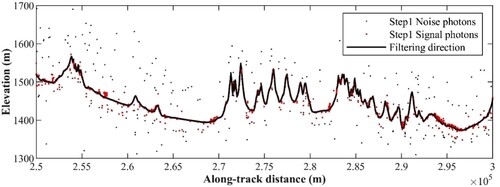

(2)	Adaptive threshold

Based on denoising result of the first-step, the elevation segment is divided into 2 m intervals along the optimal filtering direction. The density of signal photons in each elevation segment is computed, and the elevation segment with the largest density is taken as the main signal. The adaptive threshold is used to screen discrete signal photons far away from the main signal, and those larger than the threshold are signal photons. The adaptive threshold v is calculated according to Equations 5-7: (5) $N_{bins}={\displaystyle \frac{Z_{max}-Z_{min}}{Z_{bin}}}$(5) (6) $C={\displaystyle \frac{N_S+N_n}{N_n}}$(6) (7) $Thres={\displaystyle \frac{N_S+\ln (N_{bins})}{\ln (C)}}$(7) where $N_{bins}$ represents the number of elevation segments along the optimal filtering direction; $Z_{max}$ and $Z_{min}$ represent the maximum and minimum values of local elevation, respectively; $Z_{bin}$ indicates the statistical interval; $N_S$ and $N_n$represent the average number of signal and noise photons of a signal elevation segment, respectively; C represents the ratio of echo signal and noise of a single elevation segment; Thres represents the adaptive threshold.

2.3 Accuracy assessment

After the denoising process with two steps, the proposed algorithm gives the classification attributes of each photon, namely noise and signal photons. This study evaluates the algorithm’s stability and effectiveness via a combination of qualitative and quantitative analyses.

2.3.1 Qualitative analysis

The color separation compared with the raw photons indicates the signal and noise photons that are recognized by the proposed algorithm. Through visual inspections, a detailed analysis is performed in the areas with apparent differences.

2.3.2 Quantitative analysis

For MATLAS data, the official classification labels provided by MATLAS products are utilized to quantitatively assess the denoising results of the proposed method by calculating three statistical indicators, including Recall (R), Precision (P), and F-measure (F). The calculation equations are as follows: (8) $R={\displaystyle \frac{TS}{TS+FN}}$(8) (9) $P={\displaystyle \frac{TS}{TS+FS}}$(9) (10) $F={\displaystyle \frac{2PR}{P+R}}$(10) where TS represents the number of signal photons that are correctly recognized; FS represents the number of noise photons misclassified as signal photons; FN represents the number of signal photons misrecognized as noise photons; TN represents the number of noise photons that are correctly recognized. To test the applicability of the algorithm, the proposed method was compared with the random forest classification algorithm proposed by Chen et al. (2019), the PSO-DBSCAN proposed by Huang et al. (2019), and the localized statistics algorithm proposed by Xia et al. (2014).

For ATLAS data, this study takes the intersection of the extracted signal photons and the signal photons identified by ATL03 official results and assesses the proportion of the intersection points in their respective numbers.

3. Results

3.1 Denoising results of MATLAS data

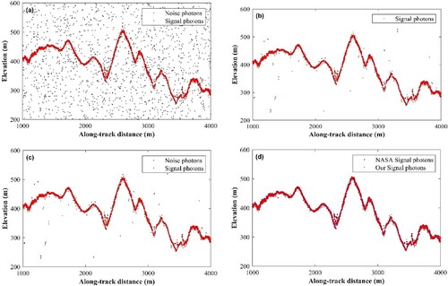
To easily evaluate the performance of the proposed denoising method, the strong beam data (t024900_010_2_8C_1VEG) of the West Coast is selected to intuitively display NASA's results, the proposed algorithm and the comparison results, respectively. As shown in Figure 4, the data contains numerous noise photons, with complex terrain. Compared with NASA signal photons, the proposed denoising method can recognize the signal photons in complicated topographical regions effectively. The comparison result indicating the performance of the proposed method in the near signal area is shown in Figure 4(d), several noise photons misrecognized as signal photons are efficiently detected.

Figure 4. Denoising results of the strong beam with complicated topography on the West Coast. (a) NASA classification result, (b) first-step denoising result of the proposed algorithm, (c) second-step denoising result of the proposed algorithm, (d) comparison between recognized signal photons and NASA signal photons.

Figure 5 and Table 3 show the quantitative evaluation results of the proposed denoising algorithm on MATLAS data. It can be seen that the F value of the first-step denoising is higher than 0.87, and the average accuracy exceeds 0.94, indicating that the first-step denoising can correctly identify most signal photons. Although the P value of some data is only 0.80, and the F value is 0.88, this ensures that the signal photons are retained to the greatest extent. The second-step denoising can improve the denoising accuracy based on the first-step, where P increases from 0.80–0.89, and the F value increases from 0.87–0.93. As presented in Figure 4(c), the signal photons misclassified in the first-step denoising are accurately removed, and the signal and noise photons are well distinguished.

Figure 5. F Value of denoising result under different conditions.

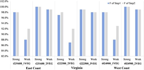
Table 3. Valuation indicators of the proposed algorithm based on MATLAS data.

Dataset	Beam	Noise Number	Signal Number	First-step denoising			Second-step denoising
				R	P	F	R	P	F
t231600_010_2_8B_1VEG	Strong	25323	19902	0.99	0.96	0.98	0.99	0.97	0.98
	Weak	25323	5125	0.95	0.81	0.88	0.95	0.90	0.92
t231600_010_2_8B_2VEG	Strong	1863	20106	0.99	1.00	1.00	0.99	1.00	1.00
	Weak	1863	5075	0.99	0.98	0.99	0.99	0.99	0.99
Mean	–	–	0.98	0.94	0.96	0.98	0.96	0.97
t222500_010_2_8a_2VEG	Strong	26053	28633	0.97	0.97	0.97	0.97	0.98	0.98
	Weak	26053	7223	0.95	0.80	0.87	0.95	0.89	0.92
t222500_010_2_8a_3VEG	Strong	1852	28588	0.98	1.00	0.99	0.97	1.00	0.99
	Weak	1852	7280	0.97	0.99	0.98	0.97	0.99	0.98
Mean	–	–	0.97	0.94	0.95	0.96	0.97	0.96
t024900_010_2_8C_1VEG	Strong	23870	18762	0.99	0.96	0.98	0.99	0.97	0.98
	Weak	23870	4869	0.97	0.80	0.88	0.97	0.89	0.93
t024900_010_2_8C_2VEG	Strong	1707	19002	1.00	1.00	1.00	1.00	1.00	1.00
	Weak	1707	4709	1.00	0.98	0.99	1.00	0.98	0.99
Mean	–	–	0.99	0.94	0.96	0.99	0.96	0.97

The comparison between the accuracy differences under various observation conditions indicates that the accuracy under the low background noise is significantly higher than that under the high background noise. For example, the F values corresponding to the strong beam of t231600_1VEG and t231600_2VEG are 0.98 and 1.00 respectively. This influence is especially apparent in weak beam data, where the F value of the t231600_2VEG data is 0.7 higher than that of t231600_1VEG. Because there are many noise photons in the atmosphere under the high background noise, and some of the noise photons are very similar to the signal photons in terms of distribution, which makes it challenging to identify, resulting in the low denoising accuracy.

Under different beam conditions, a higher SNR has a better denoising effect. For example, in the West Coast area, the SNR of four data from small to large is: t024900_1VEG weak beam data (0.20) < t024900_ 1VEG strong beam data (0.79) < t024900_ 2VEG weak beam data (2.76) < t024900_ 2VEG strong beam data (11.13), with corresponding F values are 0.93, 0.98, 0.99 and 1.00, respectively.

Besides, the algorithm can perform photon denoising well with a P-value of 0.80-1.00 and an F-value of 0.87-1.00 in different vegetation coverage and topography areas.

3.2 Denoising results of the ATLAS data

Figures 6 and 7 show the denoising results of the proposed algorithm on data A and B, respectively. As in the case of MATLAS data, the first-step denoising based on density and curvature features significantly reduces the number of noise photons, but there still exist a certain amount of dense local noise photons caused by random noise. Compared with Figures 6(a), (c) and 7(a), (c), the second-step denoising results shown in Figures 6(b), (d) and 7(b), (d) effectively remove the residual noise photons. The signal photons are continuous and concentrated, and the visual effect is suitable for daytime or nighttime and under strong or weak beam observation conditions.

Figure 6. Denoising results of data A under nighttime observation. (a) first-step denoising result of Data A_gt1 l, (b) final denoising result of Data A_gt1 l, (c) first-step denoising result of Data A_gt1r, (d) final denoising result of Data A_gt1r.

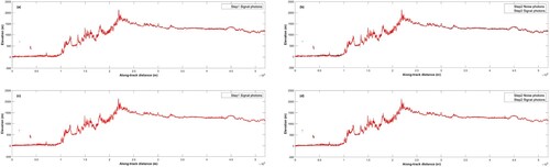
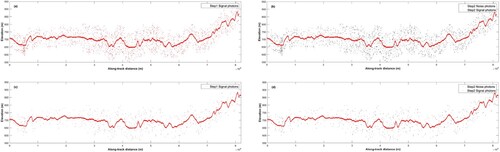
Figure 7. Denoising results of data A under nighttime observation. (a) first-step denoising result of Data B_gt1 l, (b) final denoising result of Data B_gt1 l, (c) first-step denoising result of Data B_gt1r, (d) final denoising result of Data B_gt1r.

To further evaluate the algorithm’s accuracy, the denoising results of ATLAS data are quantitatively analysed. Due to the lack of reference results for verifying the denoising effect, the elevation products as a comparison will also cause significant deviations as a result of differences in time or errors in further data processing (Zhang et al. 2022). This study evaluated the denoising accuracy by taking an intersection of the signal photons recognized by the proposed algorithm and ATL03 results, and subsequently analysed the proportion of intersections to each other. In the ATL03 results, those with a confidence level greater than one are taken as signal photons.

As shown in Table 4, the number of signal photons identified in this study is higher than that in the ATL03 results under nighttime observations, and the intersection of ATL03 signal photons and those identified in this study can both account for more than 99%, indicating that the ATL03 results are highly compatible with the results in this study. On the contrary, the number of signal photons identified by the proposed method is smaller than that in the ATL03 results during daytime observation, and there is a large variation in the proportion of intersection photons under strong and weak beams. Under daytime/weak beam conditions, the intersection of photons accounts for 99.51% of signal photons identified in this study but only 88.12% of ATL03 signal photons. Under daytime/strong beam conditions, the proportion is 99.98% and 97.85%, respectively. The possible reason lies in the high background noise level, given that the signal photons’ density has no apparent advantage over noises under daytime/weak beam conditions. Accordingly, the ATL03 denoising algorithm cannot correctly recognize the noise photons close to signal photons and areas with inconsistent background noise levels, while the proposed algorithm can still achieve relatively good robustness and adaptability. As shown in Figure 8, some noise photons are misrecognized as signal photons in the ATL03 results. The signal photons identified in this study conform to the distribution characteristics of point cloud, demonstrating the credibility of the results in this study.

Figure 8. Partial visual analysis of Data B based on the ATL03 algorithm and the proposed method. (a) denoising result of the ATL03 using Data B_gt1 l, (b) denoising result of the proposed method using Data B_gt1 l, (c) denoising result of the ATL03 using Data B_gt1r, (d) denoising result of the proposed method using Data B_gt1r.

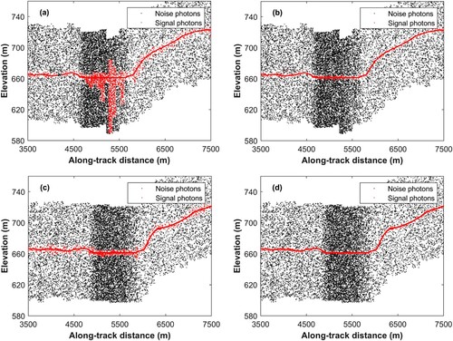
Table 4. Comparison between the results in this study and ATL03.

Data	SNR	Time/Beam	Method	First-step denoising			Second-step denoising
				Num. of Intersection	Num. of signal	Rate/%	Num. of Intersection	Num. of signal	Rate/%
Data A_gt1l	56.71	Nighttime/Weak	ATL03	346,890	347,060	99.95	345,785	347,060	99.63
			Proposed algorithm		349,470	99.26		347,176	99.60
Data A_gt1r	71.79	Nighttime/Strong	ATL03	1,418,469	1,421,291	99.80	1,418,085	1,421,291	99.77
			Proposed algorithm		1,422,115	99.74		1,421,411	99.77
Data B_gt1l	0.38	Daytime/Weak	ATL03	63,203	76,772	82.33	67,651	76,772	88.12
			Proposed algorithm		67,882	93.11		67,985	99.51
Data B_gt1r	1.32	Daytime/Strong	ATL03	260,021	265,847	97.81	260,136	265,847	97.85
			Proposed algorithm		261,157	99.57		260,197	99.98

In summary, the qualitative and quantitative evaluation results indicate that the proposed method can maintain a high recognition rate and accuracy for point cloud data with different terrains and surface types under different observation conditions (i.e. daytime/nighttime acquisition or strong/weak beam). The accuracy is effectively improved with the number of denoising times, and the maximum number of signal photons that can be recognized is retained in the final products. However, the denoising effect will be affected for photons with a low SNR, degrading the recognition rate and accuracy.

4. Discussion

4.1 Comparison of denoising results with different parameters

This algorithm should adjust the parameter K to represent the number of selected neighboring photons, whose significance lies in the measurement of the point density. Quantitative comparisons are conducted to investigate the denoising results of different K values as presented in Figure 9.

Figure 9. Comparison of denoising results with different K values.

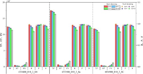
In the first-step denoising process, the TP and FP values gradually decrease with the increase of the K value. Conversely, the TN and FN values increase accompanied by the decrease of R, the increase of P, and the gradual decrease in the F-value. The number of adjacent photons within the search radius is reserved when it is greater than the specified K value; otherwise, they will be distinguished as noises. Under a small value of K, although more noise photons are easily recognized as signal photons, these misidentified signal photons will be further removed in the second-step denoising process. Besides, in the area where the signal photons are sparse, a significantly large value of K tends to recognize the signal photons as noise photons. The quantitative analysis of the relationship between the K value and the classification accuracy indicates that the denoising accuracy gradually decreases with the increase of K value, and the increase in K value is not compensated.

4.2 Analysis of denoising results in different scenes

In order to assess the applicability of the proposed algorithm in complex surface types and topographies, some typical terrains and surface types, including mountains/vegetation, flat terrain/buildings and shallow waters, are selected from data A. Areas that cannot be identified by the ATL03 results are visually analysed using the Google Earth images to validate the actual surface types. The results are shown in Figure 10.

Figure 10. Experimental results of different scenarios in data A.

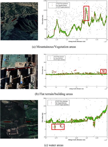
Figure 10 shows that although the ATL03 results are highly compatible with the results of this study, the ATL03 algorithm cannot effectively identify signal photons for some mountainous area withs large slopes (Figure 10(a)) or building areas with sudden changes in ground elevation (Figure 10(b)). The possible reason is that the ATL03 algorithm employs the local elevation histogram for denoising with a specific threshold (Neumann et al. 2021). Accordingly, the signal photons exceeding the threshold are misclassified as noise photons.

4.3 Denoising results of different algorithms

In order to further evaluate the performance of the proposed denoising method, it is compared with other representative algorithms using supervised and unsupervised classification procedures. For the random forest classification algorithm proposed by Chen et al. (2019), the accuracy of noise photons and signal photons at high noise rate in Virginia area are shown in Table 5: R = 0.96, P = 0.94, F = 0.95 and R = 0.94, P = 0.96, F = 0.95, respectively. While the proposed algorithm achieved a higher denoising accuracy, in which the accuracy of noise photons and signal photons are R = 0.98, P = 0.97, F = 0.97 and R = 0.97, P = 0.98, F = 0.98, respectively.

Table 5. Statistical indicators of supervised classification algorithm.

Method	Photon Class	Statistical indicators
		R	P	F
RF	Signal	0.94	0.96	0.95
	Noise	0.96	0.94	0.95
Proposed algorithm	Signal	0.98	0.97	0.97
	Noise	0.97	0.98	0.98

Table 6 lists the statistical indicators of unsupervised classification algorithms under different beam intensities and SNR. The results show that all algorithms provide good denoising performance under strong beams, regardless of the strong or weak background noise levels, and each accuracy indicator exceeds 0.88. In the case of a weak beam, the algorithm of localized statistics has a wide range of F values from 0.21–0.88 under different background noise levels. The possible reason is that the local distance statistical algorithm relies on manual parameter adjustment, which makes the algorithm only applicable to a specific environment rather than complex regions with different photon density characteristics. In contrast, since the proposed algorithm and the PSO-DBSCAN algorithm do not need to adjust parameters manually, the results can meet the denoising requirements of weak beam data with different background noise levels and the proposed method has a higher P value (0.96) and F value (0.96) than PSO-DBSCAN.

Table 6. Statistical indicators of unsupervised classification algorithm under different beam intensities (Huang et al. 2019, 2020).

Beam	Dataset	SNR	Localized Statistics			PSO-DBSCAN			Proposed algorithm
			R	P	F	R	P	F	R	P	F
Strong	t231600_010_2_8B_2VEG	10.79	1.00	0.99	0.99	1.00	1.00	1.00	0.99	1.00	1.00
	t222500_010_2_8a_2VEG	1.09	1.00	0.92	0.96	1.00	0.97	0.98	0.97	0.98	0.98
	t222500_010_2_8a_3VEG	15.44	1.00	0.88	0.94	1.00	0.99	1.00	0.97	1.00	0.99
	Mean		1.00	0.93	0.96	1.00	0.99	0.99	0.98	0.99	0.99
Weak	t231600_010_2_8B_2VEG	2.72	0.12	1.00	0.21	1.00	0.99	0.99	0.99	0.99	0.99
	t222500_010_2_8a_2VEG	0.27	0.55	0.80	0.66	1.00	0.82	0.90	0.95	0.89	0.92
	t222500_010_2_8a_3VEG	3.93	0.92	0.85	0.88	1.00	0.82	0.90	0.97	0.99	0.98
	Mean		0.53	0.88	0.58	1.00	0.88	0.93	0.97	0.96	0.96

5. Conclusion

Since the existing algorithms cannot meet the denoising requirements of the photon-counting LiDAR data with different surface types under different observation conditions, this study proposes an adaptive denoising method for photon point cloud to address the aforementioned challenges. Some conclusions are drawn from the experiments on the MATLAS and ICESat-2/ATLAS data:

1. The proposed denoising algorithm is applied to data denoising with different surface types, observation conditions, and inconsistent noise levels, considering the noise level, spatial density, and terrain of the photon point cloud. Unlike the mainstream denoising algorithms, the proposed algorithm adds local curvature and directional features in addition to traditional statistical parameters such as elevation and density. The supplementary features can better reflect the morphological characteristics of point cloud clusters, making the proposed algorithm more suitable for the distribution characteristics of scattered photon point clouds with different surface types and observation conditions.

2. In response to the influence of noise unevenness during the daytime, a dynamic neighborhood radius is calculated adaptively according to the area and the number of photons of each along-track segment, which is more targeted and adaptable than the fixed threshold. The dynamic neighborhood radius can accurately capture the local curvature information under different noise levels, thereby increasing the discriminability of signal and noise photons.

3. This study adopts the RANSAC algorithm to find the optimal filtering direction of the neighborhood area, rather than the direction of maximum density obtained by traversing different directions or using principal component analysis.

4. The results demonstrate that the high accuracy and universality of the proposed algorithm by leveraging the MATLAS data covering different terrains and SNR to perform denoising experiments. Specifically, the average F value of the first-step denoising exceeds 0.87. After the second-step denoising, the average F value can reach 0.92.

5. The comparison between the denoising results of this study and the official ATL03 reference data indicates that the proposed method can perform well for photons with different surface types and topographies under various observation conditions.

However, in the along-track direction, when the same feature is divided into different windows, some signal photons are misrecognized as noise photons due to photon density and noise threshold. In the future, the proposed method can be combined with the regional growth method and overlapping moving window to solve the deficiencies of the proposed denoising algorithm. Additionally, the processing efficiency is another important indicator to evaluate the algorithm, we should focus on how to evaluate the complexity of the algorithm.

Acknowledgements

We are grateful to the NSIDC for providing the ATL03 data and the NASA for providing the MATLAS data. We also would like to thank the editors and anonymous reviewers for their valuable comments on this letter.

Data availability statement.

The data that support the findings of this study are available from the corresponding author upon reasonable request.

Disclosure statement

No potential conflict of interest was reported by the author(s).

Additional information

Funding

This work was supported by the National Key R&D Program of China under [grant number 2021YFF0704600]; the National Natural Science Foundation of China under [grant number 42171352, 42271365, U22A20566]; and the High-Level Talent Aggregation Project in Hunan Province, China-Innovation Team under [grant number 2019RS1060].

References

- Cao, J. J., H. Chen, J. Zhang, Y. J. Li, X. P. Liu, and C. Q. Zhou. 2018. “Normal Estimation via Shifted Neighborhood for Point Cloud.” Journal of Computational and Applied Mathematics 329: 57–67. doi:10.1016/j.cam.2017.04.027.
- Chen, B. W., Y. Pang, Z. Y. Li, H. Lu, and X. J. Liu. 2019. “Photon-counting LiDAR Point Cloud Data Filtering Based on the Random Forest Algorithm.” Journal of Geo-Information Science 21 (6): 898–906. doi:10.12082/dqxxkx.2019.190013.
- Chen, F., N. Wang, B. Yu, and L. Wang. 2022. “Res2-Unet, A New Deep Architecture for Building Detection from High Spatial Resolution Images.” IEEE Journal of Selected Topics in Applied Earth Observations and Remote Sensing 15: 1494–1501. doi:10.1109/JSTARS.2022.3146430.
- Chen, B., B. Xu, and P. Gong. 2021. “Mapping Essential Urban Land use Categories (EULUC) Using Geospatial big Data: Progress, Challenges, and Opportunities.” Big Earth Data 5 (3): 410–441. doi:10.1080/20964471.2021.1939243.
- Gong, P., L. Zhan, H. B. Huang, G. Q. Sun, and L. Wang. 2011. “ICESat GLAS Data for Urban Environment Monitoring.” IEEE Transactions on Geoscience and Remote Sensing 49 (3): 1158–1172. doi:10.1109/TGRS.2010.2070514.
- Guo, H. D., D. Liang, F. Cheng, and Z. Shirazi. 2021. “Innovative Approaches to the Sustainable Development Goals Using Big Earth Data.” Big Earth Data 5 (3): 263–276. doi:10.1080/20964471.2021.1939989.
- Gwenzi, D., M. A. Lefsky, V. P. Suchdeo, and D. J. Harding. 2016. “Prospects of the Icesat-2 Laser Altimetry Mission for Savanna Ecosystem Structural Studies Based on Airborne Simulation Data.” ISPRS Journal of Photogrammetry and Remote Sensing 118: 68–82. doi:10.1016/j.isprsjprs.2016.04.009.
- Herzfeld, U. C., B. W. McDonald, B. F. Wallin, T. A. Neumann, T. Markus, A. Brenner, and C. Field. 2014. “Algorithm for Detection of Ground and Canopy Cover in Micro-Pulse Photon-Counting Lidar Altimeter Data in Preparation for the ICE-Sat-2 Mission.” IEEE Transactions on Geoscience and Remote Sensing 52 (4): 2109–2125. doi:10.1109/TGRS.2013.2258350.
- Herzfeld, U. C., T. M. Trantow, D. Harding, and P. W. Dabney. 2017. “Surface-Height Determination of Crevassed Glaciers—Mathematical Principles of an Autoadaptive Density-Dimension Algorithm and Validation Using ICESat-2 Simulator (SIMPL) Data.” IEEE Transactions on Geoscience and Remote Sensing 55 (4): 1874–1896. doi:10.1109/TGRS.2016.2617323.
- Huang, J. P., Y. Q. Xing, L. Qin, and J. M. Ma. 2020. “Accuracy of Photon Cloud Noise Filtering Algorithm in Forest Area Under Weak Beam of Conditions.” Transactions of the Chinese Society for Agricultural Machinery 51 (4): 164–172. doi:10.6041/j.issn.1000-1298.2020.04.019.
- Huang, J. P., Y. Q. Xing, H. T. You, L. Qin, and J. M. Ma. 2019. “Particle Swarm Optimization-Based Noise Filtering Algorithm for Photon Cloud Data in Forest Area.” Remote Sensing 11 (8): 980. doi:10.3390/rs11080980.
- Lao, J. Y., C. Wang, X. X. Zhu, X. H. Xi, S. Nie, J. L. Wang, F. Cheng, and G. Q. Zhou. 2021. “Retrieving Building Height in Urban Areas Using ICESat-2 Photon-Counting LiDAR Data.” International Journal of Applied Earth Observation and Geoinformation 104: 102596. doi:10.1016/j.jag.2021.102596.
- Ma, Y., R. Liu, S. Li, W. H. Zhang, F. L. Yang, and D. P. Su. 2018. “Detecting the Ocean Surface from the raw Data of the MABEL Photon-Counting Lidar.” Optics Express 26: 24752–24762. doi:10.1364/OE.26.024752.
- Magruder, L. A., M. E. Wharton III, K. D. Stout, and A. L. Neuenschwander. 2012. “SPIE Proceedings. Proc. SPIE 8379.” Laser Radar Technology and Applications XVII: 83790Q. doi:10.1117/12.919139.
- Markus, T., T. Neumann, A. Martin, W. Abdalati, K. Brunt, B. Csatho, S. Farrell, et al. 2017. “The Ice, Cloud, and Land Elevation Satellite-2 (ICESat-2): Science Requirements, Concept, and Implementation.” Remote Sensing of Environment 190: 260–273. doi:10.1016/j.rse.2016.12.029.
- Mulverhill, C., N. C. Coops, T. Hermosilla, J. C. White, and M. A. Wulderb. 2022. “Evaluating ICESat-2 for Monitoring, Modeling, and Update of Large Area Forest Canopy Height Products.” Remote Sensing of Environment 271: 112919. doi:10.1016/j.rse.2022.112919.
- Neuenschwander, A., and K. Pitts. 2019. “The ATL08 Land and Vegetation Product for the ICESat-2 Mission.” Remote Sensing of Environment 221: 247–259. doi:10.1016/j.rse.2018.11.005.
- Neumann, T., A. Brenner, D. Hancock, J. Robbins, J. Saba, K. Harbeck, A. Gibbons, J. Lee, S. Luthcke, and T. Rebold. 2021. “ICESat-2 Algorithm Theoretical Basis Document for Global Geolocated Photons (ATL03) Release 005.” https://nsidc.org/sites/default/files/icesat2_atl03_atbd_r005_0.pdf (accessed 1 April 2022).
- Neumann, T. A., A. J. Martino, T. Markus, S. Bae, M. R. Bock, A. C. Brenner, K. M. Brunt, et al. 2019. “The Ice, Cloud, and Land Elevation Satellite – 2 Mission: A Global Geolocated Photon Product Derived from the Advanced Topographic Laser Altimeter System.” Remote Sensing of Environment 233: 111325. doi:10.1016/j.rse.2019.111325.
- Nie, S., C. Wang, X. H. Xi, S. Z. Luo, G. Y. Li, J. Y. Tian, and H. T. Wang. 2018. “Estimating the Vegetation Canopy Height Using Micro-Pulse Photon-Counting LiDAR Data.” Optics Express 26 (10): A520–A540. doi:10.1364/OE.26.00A520.
- Popescu, S., T. Zhou, R. Nelson, A. Neuenschwander, R. Sheridan, L. Narine, and K. M. Walshd. 2018. “Photon Counting LiDAR: An Adaptive Ground and Canopy Height Retrieval Algorithm for ICESat-2 Data.” Remote Sensing of Environment 208: 154–170. doi:10.1016/j.rse.2018.02.019.
- Tang, H., A. Swatantran, T. Barrett, P. DeCola, and R. Dubayah. 2016. “Voxel-based Spatial Filtering Method for Canopy Height Retrieval from Airborne Single-Photon Lidar.” Remote Sensing 8 (9): 771–783. doi:10.3390/rs8090771.
- Wang, X., and X. L. Liang. 2022. “Photon-counting Laser Altimeter Data Filtering Based on Hierarchical Adaptive Filter for Forest Scenario.” The International Archives of the Photogrammetry, Remote Sensing and Spatial Information Sciences, 205–210. doi:10.5194/isprs-archives-XLIII-B3-2022-205-2022.
- Wang, C. H., A. Y. Wang, W. Rong, Y. L. Tao, and R. M. Fu. 2021. “光子计数激光雷达点云的自适应去噪算法.” Laser & Optoelectronics Progress 58 (14): 1428001–489. doi:10.3788/LOP202158.1428001.
- Xia, S. B., C. Wang, X. H. Xi, S. Z. Luo, and H. C. Zeng. 2014. “Point Cloud Filtering and Tree Height Estimation Using Airborne Experiment Data of ICESat-2.” National Remote Sensing Bulletin 18 (6): 1199–1207. doi:10.11834/jrs.20144029.
- Xie, F., G. Yang, R. Shu, and M. Li. 2017. “An Adaptive Directional Filter for Photon Counting Lidar Point Cloud Data.” Journal of Infrared and Millimeter Waves 36 (1): 107–113. doi:10.11972/j.issn.1001-9014.2017.01.019.
- Xing, Y. Q., A. D. Gier, J. J. Zhang, and L. H. Wang. 2010. “An Improved Method for Estimating Forest Canopy Height Using ICESat-GLAS Full Waveform Data Over Sloping Terrain: A Case Study in Changbai Mountains, China.” International Journal of Applied Earth Observation and Geoinformation 12 (5): 385–392. doi:10.1016/j.jag.2010.04.010.
- Yu, J. N., S. Nie, W. J. Liu, X. X. Zhu, D. J. Lu, W. Y. Wu, and Y. Sun.2021. Accuracy Assessment of ICESat-2 Ground Elevation and Canopy Height Estimates in Mangroves.” IEEE Geoscience and Remote Sensing Letters 19: 1–5. doi:10.1109/LGRS.2021.3107440.
- Zang, J. X., X. G. Lin, and X. L. Liang. 2017. “Advances and Prospects of Information Extraction from Point Clouds.” Acta Geodaetica et Cartographica Sinica 46 (10): 1460–1469. doi:10.11947/j.AGCS.2017.20170345.
- Zhang, J., and J. Kerekes. 2015. “An Adaptive Density-Based Model for Extracting Surface Returns from Photon-Counting Laser Altimeter Data.” IEEE Geoscience and Remote Sensing Letters 12 (4): 726–730. doi:10.1109/LGRS.2014.2360367.
- Zhang, S. T., G. Y. Li, X. Q. Zhou, J. Q. Yao, J. Q. Guo, and X. M. Tang. 2022a. “基于多特征自适应的单光子点云去噪算法.” Infrared and Laser Engineering 51 (6): 20210949. doi:10.3788/IRLA20210949.
- Zhang, X., Y. N. Zhou, and J. C. Luo. 2022b. “Deep Learning for Processing and Analysis of Remote Sensing big Data: A Technical Review.” Big Earth Data 6 (4): 527–560. doi:10.1080/20964471.2021.1964879.
- Zhu, X. X., S. Nie, C. Wang, X. H. Xi, and Z. Y. Hu. 2018. “A Ground Elevation and Vegetation Height Retrieval Algorithm Using Micro-Pulse Photon-Counting Lidar Data.” Remote Sensing 10 (12): 1962. doi:10.3390/rs10121962.
- Zhu, X. X., S. Nie, C. Wang, X. H. Xi, J. Y. Lao, and D. Li. 2022. “Consistency Analysis of Forest Height Retrievals Between GEDI and ICESat-2.” Remote Sensing of Environment 281: 113244. doi:10.1016/j.rse.2022.113244.
- Zhu, X. X., S. Nie, C. Wang, X. H. Xi, J. S. Wang, D. Li, and H. Y. Zhou. 2021. “A Noise Removal Algorithm Based on OPTICS for Photon-Counting LiDAR Data.” IEEE Geoscience and Remote Sensing Letters 18 (8): 1471–1475. doi:10.1109/LGRS.2020.3003191.
- Zwally, H. J., B. Schutz, W. Abdalati, J. Abshire, C. Bentley, A. Brenner, J. Bufton, et al. 2002. “ICESat's Laser Measurements of Polar ice, Atmosphere, Ocean, and Land.” Journal of Geodynamics 34 (3): 405–445. doi:10.1016/S0264-3707(02)00042-X.