Construction of quality evaluation indicator system for diamond discrete global grid systems

ABSTRACT

Although the uniformity of diamond discrete global grid is essential for calculations and searches, geometric deformations increase with the level of divisions. The Goodchild Criteria provides a basis for evaluating the quality of the global grid. However, some indicators in the criteria are redundant and contradictory, and the existing indicator system has limitations. Directly using the indicator system may render the evaluation of the diamond grid unreliable. In this study, we summarized the evaluation indicators for grid quality based on the Goodchild Criteria, calculated the correlations between these indicators using different diamond grid systems, and constructed reliable evaluation systems based on similarities and differences. The selected grid systems are classified into two groups: non-equal-area and equal-area grids. Their quality evaluation systems are composed of Size-Shape-Topology Factor and Geometry-Topology Factor, respectively. The proposed quality evaluation systems utilize a minimal number of indicators selected from each factor to provide a comprehensive description of the diamond grid’s characteristics. This approach simplifies the complexity of the evaluations while improving their reliability and credibility.

KEYWORDS:

• discrete global grid
• goodchild criteria
• correlation
• factor analysis
• diamond grid

1. Introduction

The Discrete Global Grid system (DGGs) is a spatial structure based on a spherical (or ellipsoidal) surface, which can be divided infinitely without changing shape (Sahr and White 1998). If the level of divisions is small enough, the DGGs can simulate the shape of the Earth’s surface (Zhou 2001). As was suggested recently by Goodchild, a DGGs-based Geographic Information System (GIS) could be the next-generation GIS (Goodchild 2018; Robertson et al. 2020). DGGs is emerging as a data model, providing a solid foundation for big data and digital Earth frameworks (Bousquin 2021; Hojati et al. 2022; Ma et al. 2021; Thompson et al. 2022), with numerous functionalities, including spatial data management, storage, integration, exploration, visualization (Breunig et al. 2020; Purss et al. 2019; Purss et al. 2017; Zhou et al. 2018). At the same time, DGGs provides a continuous and global analytical framework for regional, or even global issues (Zhou et al. 2018), such as global environmental and soil monitoring modeling (Robertson et al. 2020), Earth system modeling (Engwirda and Liao 2021; Lin et al. 2018), watershed delineation (Liao et al. 2020; Liao et al. 2023; Liao et al. 2022; Liao et al. 2022), wildfire spread modeling (Hojati and Robertson 2020), maritime risk analytics (Rawson, Sabeur, and Brito 2022), spatial prediction of sparse events (Jendryke and Mcclure 2021), Earth observation data management (Yao et al. 2020), and so on. There are four parameters determining the configurations of DGGs: (1) a base regular polyhedron; (2) grid cell shape and refinement; (3) a fixed orientation of this polyhedron relative to the Earth; (4) a projection from the plane to the Earth (Sahr and White 1998). There are many DGGs with different parameters developed by many institutions. Based on grid cell shape, the DGGs can be classified into triangle, diamond and hexagon grids. Based on the regular polyhedron, there are octahedral, cube, and icosahedral grids, among others. Based on the projection, grids may be constructed by the equal-area or equal-angle projection, and recursive or non-recursive division methods.

There are area or shape distortions in each DGGs and the grid geometric characteristics are more complex with the level of divisions (Kimerling, Sahr, and White 1999). The complex geometric characteristics are not available for large-scale and high-precision applications, nor are they suitable for comprehensive spatial analyses (Goodchild 2018). Therefore, it is necessary to accurately describe the grid geometric characteristics and distortions, and evaluate and analyze the grid quality (Wang et al. 2021; Zhou, Ou, and Ma 2009), ensuring the reliability and credibility of DGGs in multiple fields.

Currently, researchers are interested in the Goodchild Criteria, which are a general rule for DGGs (Kimerling, Sahr, and White 1999) (Appendix 1). New quantitative indicators have been developed based on the fundamental criterion to evaluate and analyze the geometric characteristics and deformations of DGGs. For example, Heikes and Randall proposed the ‘cell wall midpoint ratio’ to measure the coincidence of the midpoint of the great arc connecting two adjacent grid cell centers and the midpoint of the shared edge between two cells (Heikes and Randall 1995). White constructed an indicator of compactness, that is the ratio of grid cell’s perimeter to area, to quantify grid shape (White et al. 1998). Ming calculated the distance between two adjacent grid cell centers and angle formed by three adjacent grid cell centers to evaluate the uniformity of grid (Ming et al. 2007). Gregory considered that the ‘cell wall midpoint ratio’ and the variation coefficient of distances between any adjacent cells are important for dynamic simulations, and used the two indicators to describe geometric characteristics of DGGs (Gregory et al. 2008). Zhang constructed an indicator based on fuzzy similarity to analyze the geometric deformations of the Quaternary Triangular Mesh (QTM) model (Zhang et al. 2015).

Other researchers studied the trends of geometric deformation and spatial distributions of grid area, angle and length in various DGGs, such as the QTM model (Zhao, Sun, and Chen 2005, 2016), the approximate equal-area diamond grid (Sun and Zhou 2016) and the equal-area hexagon grid based on the Snyder projection (Ben 2005). Furthermore, Kmoch systematically compared and summarized the deformations of grid area and shape between five open-source DGGs implementations (Kmoch et al. 2022): Uber H3 (Uber 2019), Google S2 (Veach et al. 2017), rHealpix (Bowater and Stefanakis 2018; Gibb 2016), DGGRID (Sahr 2019), OpenEAGGR (Bush 2017). The rHealpix and DGGRID ISEA-based models have the highest degree of area preservation, with 99.3% of cell areas being close to the mean value. Conversely, the Uber H3 model has the smallest shape distortions due to its high compactness when compared to other grid models.

Therefore, most of the selected or constructed indicators are based on the Goodchild Criteria, and the descriptions or evaluations of grid geometric characteristics and distortions are mainly based on one or multiple indicators individually. Currently, there is no comprehensive quality evaluation system for DGGs, as the Goodchild Criteria have contradictions and redundancies, and no DGG meets all indicators from the criteria simultaneously (Kimerling, Sahr, and White 1999). Wang investigated correlations among indicators based on the Goodchild Criteria and reconstructed a geometric evaluation indicator system for the QTM model (Wang et al. 2021). The system includes two common factors: area factor and shape factor. The area factor mainly covers grid area, edge length, distance between two adjacent grid cell centers and ‘cell wall midpoint ratio’, while the shape factor mainly considers grid shape, compactness and structure. The use of this evaluation indicator system enhances the reliability and credibility of quality evaluations.

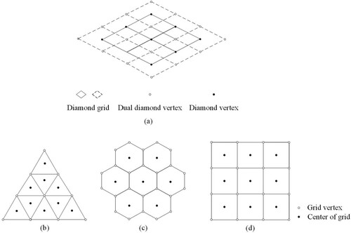
However, Wang’s evaluation system is specifically designed for the QTM model, which is a triangle grid. It cannot be used for diamond or hexagon grids due to differences in geometry between the QTM model and these grids. Blindly applying this system to other grids could significantly reduce the credibility of grid quality evaluations. Triangle grid has upper and lower triangles (Figure 1b). There are only a few algorithms that can be directly applied to triangle and hexagon grids (Figure 1c). However, the diamond grid has a simple structure, consistent orientation, radial symmetry, and translation phase harmony (Figure 1a). Additionally, some algorithms based on raster data can be directly applied to diamond grids, which are similar to pixels in raster data (Figure 1d) (Liu 2013; Lu 2016). The diamond grid is widely utilized in geospatial operations and data integration (Yuan, Zhao, and Zhao 2018), such as the integration and management of China’s ocean tidal waves data (Liu 2013).

Figure 1. Grids with different cell shape: (a) diamond; (b) triangle; (c) hexagon; (d) square.

In this paper, we will:

1. Summarize the information on grid quality evaluation indicators based on the Goodchild Criteria;

2. Calculate the correlations among these indicators based on different diamond grids;

3. Identify the similarities and differences between indicators based on different diamond grids and construct a reliable quality evaluation indicator system.

The remainder of this paper is organized as follows: in Section 2, we present the theory and methods, mainly including the construction of different diamond grids, the selection and quantification of indicators, and the modeling of the quality evaluation indicator system. In Section 3, we report the experimental results. In Section 4, we discuss the results. Finally, we provide conclusions and the future work in Section 5.

2. Theory and methods

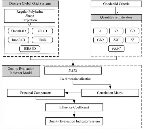
To construct quality evaluation indicator systems for diamond grid, we propose using the Factor Analysis (FA) method to calculate correlations between quantitative indicators and extracting common information. The process is illustrated in Figure 2, and the key steps are as follows:

1. Select representative discrete global grid systems. We have chosen five DGGs with varying parameters.

2. Select appropriate quantitative indicators. We have identified seven quantitative indicators from the Goodchild Criteria.

3. Construct quality evaluation indicator models. By applying the FA method to the correlation matrix of the indicators for each DGGs, we can extract the main information and construct a quality evaluation indicator system based on the influence coefficient of the principal components, using logical reasoning.

Figure 2. Flowchart of the quality evaluation indicator model. The abbreviations in Discrete Global Grid Systems are described in Table 1. The abbreviations among the Quantitative Indicators are defined in Appendix 1. DATA refers to an observation data matrix.

2.1. Discrete global grid systems

The regular octahedron and icosahedron were chosen as the base regular polyhedrons due to their consistent alignment with points on the Earth’s surface, such as, the pole, the equator, the principal meridian, and other meridians at 90°, 180°, and 270° (Zhao and Bai 2007) (Figure 3a,b). The icosahedron is preferred due to its ability to produce less distortion compared to other Platonic solids (Ali, Troy, and Faramarz 2015) (Figure 3c). The transformation from the plane to the Earth was achieved through the use of equal-area projection, recursive and non-recursive division methods. The equal-area grids ensure accuracy in area calculations (Sun and Zhou 2016), geospatial sampling uniformity, and geostatistical efficiency (Sahr, Dumas, and Choudhuri 2015). Most equal-area grids are constructed using the Snyder projection, such as the Icosahedral Snyder Equal Area aperture 3 Hexagon (ISEA3H) model (Jendryke and Mcclure 2019) and the Icosahedral Snyder Equal Area aperture 4 Diamond (ISEA4D) model (Neeraj et al. 2019). Because of their outstanding geometric properties, many researchers prefer recursive and non-recursive division methods (Wang and Lee 2011; Zhou et al. 2018). The Aperture-4 diamond grid was constructed to correspond with the quadtree structure (Figure 4). The selected grids are listed in Table 1. The regular octahedron was not studied as there is no equal-area grid available for it.

Figure 3. Regular polyhedrons: (a) octahedron; (b) spherical octahedron; (c) icosahedron.

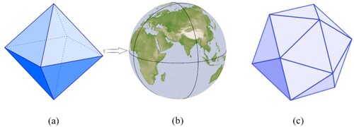
Figure 4. Diamond grids with different aperture: (a) aperture-4 diamond; (b) aperture-9 diamond.

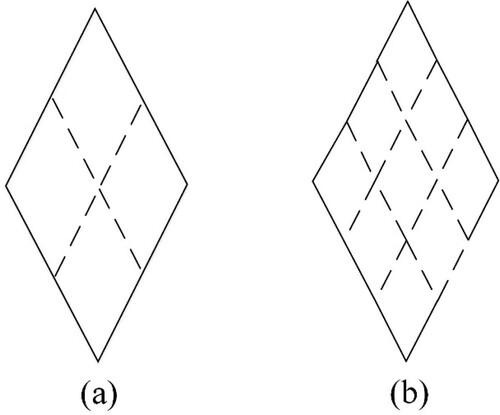
Table 1. Discrete global grid systems used this paper.

Shape	Diamond	Grids	Abbreviation
Regular polyhedron	Octahedron	Icosahedral Snyder Equal Area aperture 4 Diamond	ISEA4D
	Icosahedron	Octahedral Recursive Division aperture 4 Diamond	OR4D
Projection	Snyder	Octahedral non-Recursive Division aperture 4 Diamond	OnonR4D
	Recursive	Icosahedral Recursive Division aperture 4 Diamond	IR4D
	Non-Recursive	Icosahedral non-Recursive Division aperture 4 Diamond	InonR4D

2.2. Quantitative indicators

Seven quantitative indicators corresponding to No. 2, 4, 5, 6, 7, 10 and 11 in the Goodchild Criteria were selected to describe the geometric characteristics of grid models (Wang et al. 2021) (see Appendix 2). These indicators include Area (A), Edge (D), Centers’ Distance (CD), the ‘cell wall midpoint ratio’ (CSD), Compactness (ZSC), Fractal Dimension (FRAC) and Shape Index (SI).

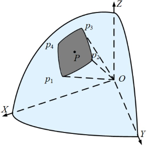
All of these indicators were calculated based on spherical geometry. For example, A is the area of a spherical polygon, while D is the geodesic distance between two points on the sphere. As shown in Figure 5, O and R are the center and radius of the sphere, respectively, and P is a spherical polygon with vertices p₁(x₁, y₁, z₁), … , p_n(x_n, y_n, z_n).

Figure 5. Spherical polygon P. Where O is the center of the sphere, p₁, p₂, p₃, p₄ are vertices of the spherical polygon P.

Indicators quantitation are as follows:

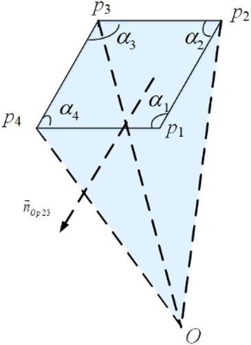
A. Any grid cell area can be calculated with formula (1). (1) $A=R^2\times \left(\sum {\alpha }_i-(N-2)\pi \right)$(1) where N is the total number of grid edge, and ${\alpha }_i=\arccos ({\overrightarrow{n}}_{Opi,i+1}\cdot {\overrightarrow{n}}_{Opi,i-1})$ $=\arccos (({\overrightarrow{Op}}_i\times {\overrightarrow{Op}}_{i-1}))$ is the dihedral angle p_i−1-O_pi-p_i + 1 (Figure 6).

Figure 6. Polygon P and its dihedral angle. p₁, p₂, p₃, p₄ are the vertices of spherical polygon P; α₁, α₂, α₃ and α₄ are the inner angles of the spherical polygon P; ${\overrightarrow{\mathit{n}}}_{\mathit{O}p23}$ is the normal vector of plane Op₂p₃.

D. The geodesic distance between two adjacent points (Figure 7) can be calculated with formula (2). (2) $d_{ij}=R\times {\theta }_{ij}=\arccos (\overrightarrow{O{p}_i}\cdot \overrightarrow{O{p}_{i+1}}/R^2)$(2)

Figure 7. Spherical distance. Where O is the center of the sphere; r is the radius of the sphere; p_i and p_j are points on the sphere; θ_ij is the angle between ${\overrightarrow{Op}}_i$ and ${\overrightarrow{Op}}_j$; d_ij is the spherical distance between p_i and p_j.

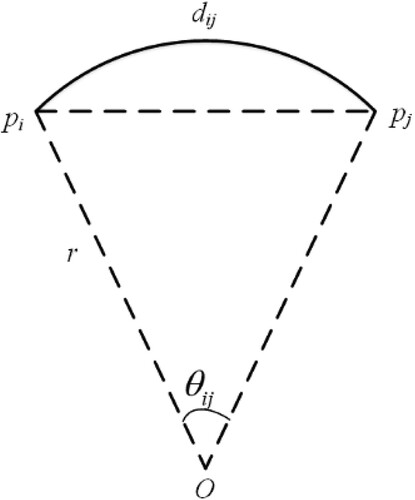
where θ_ij is the angle between ${\overrightarrow{Op}}_i$ and ${\overrightarrow{Op}}_j$.

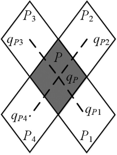
CD. As shown in Figure 8, q_P is the center of diamond grid cell P, q_Pi is the center of its adjacent grid cell P_i. The geometric center of any spherical convex polygon can be replaced by its center of gravity (Zhou et al. 2020). The geodesic distance between the two points can be calculated with formula (2). It should be pointed out that CD is just for cells sharing an edge.

Figure 8. Distance between two adjacent grid cell centers. Where q_P, q_P1, q_P2, q_P3 and q_P4 is the center of the diamond grid cell P, P₁, P₂, P₃ and P₄.

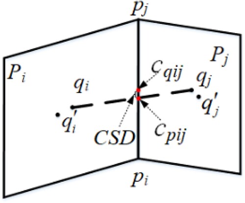
CSD. As shown in Figure 9, c_pij is the midpoint of the shared edge p_ij between grid cell P_i and P_j; c_qij is the midpoint of the line q_ij connecting grid cell centers q_i, q_j. CSD is the geodesic distance between c_pij and c_qij (formula (2)).

Figure 9. Parameters for CSD. Where q_i and q_j are the centers of grid cell P_i and P_j, respectively; p_ij is the shared edge between grid cell P_i and P_j; c_pij is the midpoint of p_ij; q_ij is the line connecting grid centers q_i and q_j; c_qij is the midpoint of q_ij; CSD is the geodesic distance between c_pij and c_qij.

ZSC. Compactness describes the regularity of one polygon. The compactness of any polygon on the plane can be extended to the sphere, and it can be calculated with formula (3) (Kimerling, Sahr, and White 1999). (3) $ZSC=\sqrt{4\pi A-A^2/R^2}/\sum D_i$(3) FRAC. Fractal dimension describes the complex of one polygon, and can be expressed with formula (4) (Li et al. 2007). (4) $FRAC=2\left(\ln \sum \frac{D_i}{\ln A}\right)$(4) SI. The shape index of one polygon comes from the field of landscape ecology, and depicts the shape characteristics of any patch in the landscape (Chen, Wu, and Li 2017). It can be obtained with formula (5) (Chen, Wu, and Li 2017). (5) $SI=\sqrt{A}/\sum D_i$(5)

2.3. Quality evaluation indicator model

Seven indicators can be integrated into independent comprehensive factors by FA. The amount of information contained in the principal components is reflected by the eigenvalue and variance in the linear combination. The larger the variance, the greater the comprehensiveness of the components. Furthermore, based on the influence coefficient of the principal components, indicators for the principal components can be determined. The component can be named and interpreted based on the meaning of indicators in any principal component.

Before constructing the quality evaluation system, it is necessary to ensure the observation data of the indicators be in the same dimension. There is a grid with m cells, l edges (m≠l), where each cell has n edges. Quantifications of A, ZSC, FRAC, SI are all vectors with 1×m. That is A = (A₁, A₂, … , A_m), ZSC = (ZSC₁, ZSC₂, … , ZSC_m), FRAC = (FRAC₁, FRAC₂, … , FRAC_m), SI = (SI₁, SI₂, … , SI_m). Quantifications of D, CD, CSD are all vectors with 1×l. That is D = (D₁, D₂, … , D_l), CD = (CD₁, CD₂, … , CD_l), CSD = (CSD₁, CSD₂, … , CSD_l). For any grid cell i, the quantifications of D, CD, CSD are all vectors with 1×n, that is D_i= (d₁, d₂, … , d_n), CD_i= (cd₁, cd₂, … , cd_n), CSD_i= (csd₁, csd₂, … , csd_n). Taking the grid cell as an object, the mean of D_i, CD_i, CSD_i are the observation data of each grid cell. The observation data matrix is as follows: (6) $DATA=(A,\overline{D},\overline{CD},\overline{CSD},ZSC,FRAC,SI)={\left(\begin{array}{c}{A}_1{A}_2\dots Am\\ {\overline{D}}_1{\overline{D}}_2\dots {\overline{D}}_m\\ {\overline{CD}}_1{\overline{CD}}_2\dots {\overline{CD}}_m\\ {\overline{CSD}}_1{\overline{CSD}}_2\dots {\overline{CSD}}_m\\ ZS{C}_{1}ZS{C}_2\dots ZS{C}_m\\ FRA{C}_{1}FRA{C}_2\dots FRA{C}_m\\ S{I}_{1}S{I}_2\dots S{I}_m\end{array}\right)}_{7\times m}$(6) where ${\overline{D}}_i$, ${\overline{CD}}_i$, ${\overline{CSD}}_i$ are the mean of D_i, CD_i, CSD_i, respectively.

The correlation matrix can be calculated from DATA. The principal components can be determined by the cumulative contribution rate of variance and the abrupt change of eigenvalue. The threshold for the cumulative contribution rate is usually set to 85%. In this study, there are different geometric characteristics and correlations among different grids. It is difficult to select a suitable threshold. Eigenvalue is mainly used to determine the principal components. The abrupt change of eigenvalue from the kth eigenvalue to the k + 1th one means that the first k components are principal ones. Indicators in each principal component can be extracted by the influence coefficients of the principal components. The quality evaluation indicator model can be constructed after naming and interpreting in line with the common characteristics among indicators.

3. Results

In this section, we take the grid at the 5th level of division as a base example and grids at the 6th, 7th and 8th level as verifiable examples, to extract the correlations between indicators and construct quality evaluation indictor systems for five grids. The hardware and software environments were as follows: the processor was Intel i5-6400QM and CPU @2.70 GHz; and RAM is 8.00 GB, the operating system was Windows 10 64-bit, the mathematical software was IBM SPSS Statistics 23 (Trial) and JASP (Version 0.14.1).

3.1. Octahedral non-recursive division aperture 4 diamond (OnonR4D) model

Original Data. The statistics of indicators and based on the 5th level of OnonR4D model (OnonR4D-5 OnonR4D) are shown in Table 2.

Table 2. Statistics of indicators of OnonR4D-5 model (R = 6371.007 km).

Indicator	Mean	Standard deviation
A	124527.824 km^2	40592.787
D	376.626 km	62.105
CD	374.607 km	63.705
CSD	6.735 km	8.067
ZSC	0.818	0.032
FRAC	0.626	0.006
SI	0.818	0.032

Principal components by FA. The correlation coefficient matrix and the contribution rate of variance are presented in Tables 3 and 4, respectively.

Table 3. Correlation coefficient matrix of the OnonR4D-5 model.

	A	D	CD	CSD	ZSC	FRAC	SI
A	1.000
D	0.978	1.000
CD	0.979	0.995	1.000
CSD	−0.427	−0.384	−0.464	1.000
ZSC	0.210	0.029	0.078	−0.352	1.000
FRAC	−0.786	−0.679	−0.714	0.517	−0.747	1.000
SI	0.211	0.030	0.079	−0.352	1.000	−0.748	1.000

Table 4. Eigenvalue and cumulative contribution rate of variance for the OnonR4D-5 model.

Components	Eigenvalue	Contribution rate of variance (%)	Cumulative contribution rate of variance (%)
1	4.201	60.013	60.013
2	2.110	30.139	90.152
3	0.669	9.562	99.714
4	0.019	0.267	99.981
5	0.001	0.015	99.996
6	1.089 × 10^−5	0.004	100
7	7.990 × 10^−9	1.141 × 10^−7	100

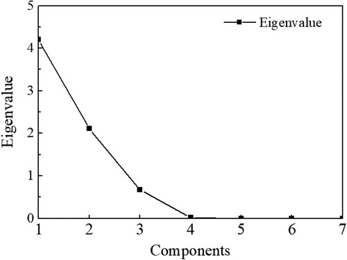
The contribution rate of the variance of the first three principal components were 60.013%, 30.139% and 9.562%, respectively, and the cumulative contribution rate of variance was more than 99.714% (Table 4). An abrupt change occurs at the 3rd eigenvalue in the curve of eigenvalues (Figure 10). That is, the first three principal components contain most of the information of all indicators.

Figure 10. Curve of eigenvalues of the OnonR4D-5 model.

Quality Evaluation Indicator System. The influence coefficient of the three components has been calculated in Table 5.

Table 5. Influence coefficient of the principal components of the OnonR4D-5 model.

Components	A	D	CD	CSD	ZSC	FRAC	SI
1	0.971	0.991	0.976	−0.266	0.023	−0.716	0.024
2	0.169	−0.010	0.030	−0.226	0.991	−0.666	0.991
3	−0.138	−0.131	−0.211	0.937	−0.130	0.190	−0.130

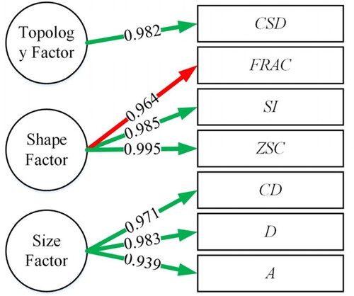
Indicators A, D, CD and FRAC with coefficients of 0.971, 0.991, 0.976 and −0.716, respectively, influence the first principal component. Indicators ZSC and SI, with a coefficient of 0.991, have a strong influence on the second principal component. The indicator CSD, with a coefficient of 0.937, greatly affects the third principal component. To illustrate the relationship between these indicators and the principal components, a path diagram has been created with the corresponding influence coefficients (Figure 11). The meaning of these indicators reveals that indicators A, D, CD and FRAC are related to the size of the grid cell, therefore the first component can be named the Size Factor. Indicators ZSC and SI are related to the shape of the grid cell, thus the second component can be referred to as the Shape Factor. Lastly, the indicator CSD represents the topology of the grid cell, making the third component the Topology Factor. In summary, the quality evaluation indicator system based on the OnonR4D model is composed of the Size-Shape-Topology Factor.

Figure 11. Path diagrams of the OnonR4D-5 Model. The green and red arrow indicate the positive and negative, respectively, and the number on each of arrows represent the absolute value of the influence coefficients of the principal components of the OnonR4D-5 model (similarly hereinafter).

The above process is repeated for the 6th, 7th and 8th level of the OnonR4D model for verification. Details of the calculation are similar to the above, and the results about the eigenvalue, (cumulative) contribution rate of variance, influence coefficient of each factor for principal components and path diagram are all expressed in Appendix 2 (Tables A2–A4 and Figure A1). These results are similar to the 5th level of the OnonR4D model because the division is consistent and preserves the overall pattern and relationships between cells. This results in a self-similar structure at different levels of geometric characteristics, with each level having the same basic geometric characteristics as the original grid.

3.2. Octahedral recursive division aperture 4 diamond (OR4D) model

The above process is carried out for the OR4D model.

Principal components by FA. The correlation matrix based on the 5th level of the OR4D model (OR4D-5 model) is shown in Table 6. The OnonR4D models showed similar results, with the first three principal components containing the majority of the indicator information (Table 7).

Table 6. Correlation matrix of the OR4D-5 model.

	A	D	CD	CSD	ZSC	FRAC	SI
A	1.000
D	0.870	1.000
CD	0.858	0.964	1.000
CSD	−0.128	0.007	−0.178	1.000
ZSC	0.213	−0.294	−0.245	−0.277	1.000
FRAC	−0.554	−0.076	−0.116	0.291	−0.930	1.000
SI	0.213	−0.294	−0.244	−0.277	1.000	−0.930	1.000

Table 7. Eigenvalue and cumulative contribution rate of variance for the OR4D-5 model.

Components	Eigenvalue	Contribution rate of variance (%)	Cumulative contribution rate of variance (%)
1	3.182	45.455	45.455
2	2.892	41.316	86.771
3	0.900	12.864	99.635
4	0.024	0.339	99.974
5	0.002	0.023	99.997
6	0.000	0.003	100.000
7	3.180 × 10^−9	4.543 × 10^−8	100.000

Quality Evaluation Indicator System. The influence coefficient of each indicator in the three components has been calculated in Table 8.

Table 8. Influence coefficients of the principal components of the OR4D-5 model.

Components	A	D	CD	CSD	ZSC	FRAC	SI
1	0.939	0.983	0.971	−0.062	−0.129	−0.243	−0.128
2	0.338	−0.165	−0.140	−0.179	0.985	−0.964	0.985
3	−0.007	0.041	−0.148	0.982	−0.112	0.105	−0.112

Indicators A, D and CD with the coefficients of 0.939, 0.983 and 0.971, respectively, strongly influence on the first principal component; indicators ZSC, SI and FRAC with the coefficients of 0.985 and 0.964, respectively, have a great influence on the second principal component; the third principal component is greatly influenced by the indicator CSD, with a coefficient of 0.982. The path diagram is shown in Figure 12. The quality evaluation system based on the OR4D model, which, like the OnonR4D model system, consists of a Size-Shape-Topology Factor. Similar results were obtained for the 6th, 7th and 8th levels of the OR4D model. Appendix 2 provides additional details, including eigenvalues, (cumulative) contribution rates of variance, influence coefficients of each factor for principal components, and the path diagrams (see Tables A5–A8 and Figure A2).

Figure 12. Path diagram of the OR4D-5 model.

3.3. Icosahedral non-recursive division aperture 4 diamond (InonR4D) model

Repeat the same process as the OnonR4D and OR4D models for the InonR4D model.

Principal components by FA. The correlation matrix for the InonR4D-5 model, which is based on the 5th level of the InonR4D model. Similar to the OnonR4D and OR4D models, the first three principal components of this correlation matrix (Table 9) contain most of the indicators’ information (Table 10).

Table 9. Correlation matrix of the InonR4D-5 model.

	A	D	CD	CSD	ZSC	FRAC	SI
A	1.000
D	0.981	1.000
CD	0.981	0.992	1.000
CSD	−0.460	−0.442	−0.541	1.000
ZSC	0.097	−0.092	−0.044	−0.127	1.000
FRAC	−0.817	−0.698	−0.727	0.436	−0.647	1.000
SI	0.098	−0.091	−0.043	−0.127	1.000	−0.648	1.000

Table 10. Eigenvalue and cumulative contribution rate of variance for the InonR4D-5 model.

Components	Eigenvalue	Contribution rate of variance (%)	Cumulative contribution rate of variance (%)
1	4.012	57.310	57.310
2	2.279	32.563	89.873
3	0.703	10.046	99.918
4	0.004	0.053	99.971
5	0.002	0.028	99.999
6	7.413 × 10^−5	0.001	100.000
7	6.279 × 10^−8	8.970 × 10^−7	100.000

Quality Evaluation Indicator System. The influence coefficients of each indicator in the three principal components have been calculated in Table 11. Similar to the OnonR4D models, indicators A, D, CD and FRAC, as well as ZSC and SI, and CSD have a significant impact on the three principal components, respectively. These influences are clearly illustrated in the path diagram (Figure 13).

Figure 13. Path diagrams of the InonR4D-5 model.

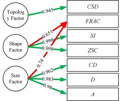
Table 11. Influence coefficients of the principal components of the InonR4D-5 model.

Components	A	D	CD	CSD	ZSC	FRAC	SI
1	0.980	0.983	0.962	−0.305	−0.014	−0.740	−0.013
2	0.103	−0.085	−0.042	−0.09	0.998	−0.651	0.998
3	−0.16	−0.158	−0.265	0.945	−0.044	0.16	−0.044

Similar to the OnonR4D and OR4D models, the evaluation system for the InonR4D model consists of a Size-Shape-Topology Factor. The above process was repeated for the 6th, 7th and 8th level of the InonR4D model, and similar conclusions have been obtained (Tables A8–A10 and Figure A3 in Appendix 2).

3.4. Icosahedral recursive division aperture 4 diamond (IR4D) model

The same process is repeated for the 5th level IR4D model (IR4D-5 model).

Principal components by FA. A correlation matrix based on the original data of the IR4D model is presented in Table 12. The results by FA based on the correlation matrix have been calculated (Table 13). Similar to the previous models, the first three principal components of the IR4D model contain the majority of the information conveyed by the seven indicators.

Table 12. Correlation matrix of the IR4D-5 model.

	A	D	CD	CSD	ZSC	FRAC	SI
A	1.000
D	0.833	1.000
CD	0.810	0.961	1.000
CSD	−0.205	−0.150	−0.339	1.000
ZSC	0.107	−0.461	−0.428	−0.063	1.000
FRAC	−0.467	0.101	0.080	0.135	−0.929	1.000
SI	0.107	−0.461	−0.428	−0.063	1.000	−0.929	1.000

Table 13. Eigenvalue and cumulative contribution rate of the variance for the IR4D-5 model.

Components	Eigenvalue	Contribution rate of variance (%)	Cumulative contribution rate of variance (%)
1	3.431	49.018	49.018
2	2.625	37.500	86.518
3	0.918	13.119	99.636
4	0.025	0.361	99.997
5	0.000	0.002	99.999
6	6.186 × 10^−5	0.001	100.000
7	1.560 × 10^−8	2.229 × 10^−7	100.000

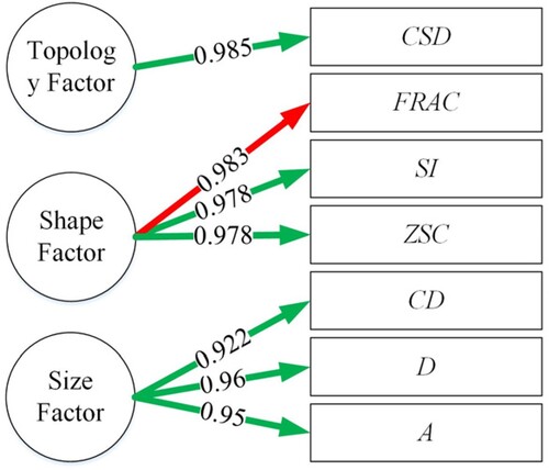
Quality Evaluation Indicator System. The influence coefficient of each indicator in the three components has been calculated in Table 14.

Table 14. Influence coefficients of the principal components of the IR4D-5 model.

Components	A	D	CD	CSD	ZSC	FRAC	SI
1	0.95	0.96	0.922	−0.144	−0.202	−0.173	−0.202
2	0.304	−0.274	−0.254	−0.066	0.978	−0.983	0.978
3	−0.049	−0.03	−0.226	0.985	−0.029	0.046	−0.029

The information coverage for these indicators by three common factors is almost complete. The indicators A, D and CD strongly influence the first principal component with coefficients of 0.95, 0.96 and 0.922, respectively; the second principal component is mostly influenced by indicators ZSC, FRAC and SI with the coefficients of 0.978, −0.983 and 0.978, respectively; the third principal component can be described by the indicator CSD, with a coefficient of 0.985. The path diagram in Figure 14 illustrates the evaluation system for the IR4D model, which is similar to the OnonR4D, OR4D and InonR4D models. The system consists of the Size-Shape-Topology Factor. The above process was repeated for the 6th, 7th and 8th level of the IR4D model, and the results are consistent with those of the 5th level grid (Tables A11–A13 and Figure A4 in Appendix 2).

Figure 14. Path diagrams of the IR4D-5 model.

3.5. Icosahedral snyder equal area aperture 4 diamond (ISEA4D) model

Original Data. As the ISEA4D model is an equal-area grid, indicators other than A were used to validate the results. The statistics for the 5th level of the ISEA4D model (ISEA4D-5 model) are represented in Table 15.

Table 15. Statistics of indicators for the ISEA4D-5 model (R = 6371.007 km).

Indicator	Mean	Standard Deviation
A	49811.716 km^2	0
D	241.173 km	7.048
CD	240.599 km	7.391
CSD	2.052 km	3.953
ZSC	0.821	0.024
FRAC	0.282	0.004
SI	0.821	0.024

Principal components by FA. All indicators are highly correlated with each other, except for CSD (Table 16). The first two principal components of the data explain 80.925% and 17.634% of the total variance, respectively, and the cumulative contribution rate of variance is over 98.559% (Table 17). The curve of eigenvalues (Figure 15) exhibits an abrupt change at the second eigenvalue, including that the first two principal components contain most of the information from all indicators.

Figure 15. Curve of eigenvalues for the ISEA4D-5 model.

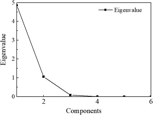
Table 16. Correlation matrix of the ISEA4D-5 model.

	D	CD	CSD	ZSC	FRAC	SI
D	1.000
CD	0.894	1.000
CSD	−0.074	−0.363	1.000
ZSC	−1.000	−0.894	0.073	1.000
FRAC	−1.000	−0.894	0.074	1.000	1.000
SI	−1.000	−0.894	0.073	1.000	1.000	1.000

Table 17. Eigenvalue and cumulative contribution rate of the variance for the ISEA4D-5 model.

Components	Eigenvalue	Contribution rate of variance (%)	Cumulative contribution rate of variance (%)
1	4.856	80.925	80.925
2	1.058	17.634	98.559
3	0.086	1.435	99.994
4	0.000	0.006	100
5	2.169 × 10^−7	3.615 × 10^−6	100
6	2.242 × 10^−8	3.737 × 10^−7	100

Quality Evaluation Indicator System. The influence coefficient of each indicator in the two components has been calculated in Table 18.

Table 18. Influence coefficients of the principal components for the ISEA4D-5 model.

Components	D	CD	CSD	ZSC	FRAC	SI
1	−0.998	−0.903	0.046	0.998	0.998	0.998
2	−0.023	−0.345	0.995	0.023	0.023	0.023

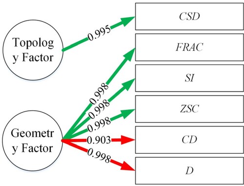
The information coverage of two principal components for each indicator is over 0.98, suggesting that there are two common factors that cover almost all the indicator information. The first component is mainly represented by the D, CD, ZSC, FRAC and SI indicators, with coefficients of −0.998, −0.903, 0.998, 0.998 and 0.998, respectively. The second component is only described by the CSD indicator, with a coefficient of 0.995. The path diagram for the two principal components is depicted in Figure 16. Based on the meaning of the indicators, the D, CD, ZSC, FRAC and SI indicators in the first component describe the geometric characteristics of the grid cell, while CSD in the second component indicates the topology of the grid cell. Thus, it can be concluded that the ISEA4D model differs from other models, and comprises a Geometry-Topology Factor. The same process was repeated to the 6th, 7th and 8th level of the ISEA4D model, yielding similar results (Tables A14–A16 and Figure A5 in Appendix 2).

Figure 16. Path diagrams of the ISEA4D-5 model.

4. Discussion

The correlations among seven quantitative indicators based on the five diamond DGGs have been calculated, and quality evaluation indicator systems have been constructed using the FA method. One system is composed of Size-Shape-Topology Factor for the non-equal-area grid model, while the other is composed of Geometry-Topology Factor for the equal-area grid model. The FA method is a dimensionality reduction technique used to analyze data with multiple variables. In this study, the seven quantitative indicators can be categorized into two or three groups based on the correlation coefficient matrices. Indicators within the same group display a strong correlation, while those in different groups exhibit a weak correlation.

In the Size Factor, the area of any spherical polygon is strongly related to its inner angles according to the Law of Sines. Additionally, due to the duality of diamonds, there is a strong correlation between a diamond's side length and its dual side length. This implies that indicators A, D and CD are related to each other. In the Shape Factor, formulas (3)–(5) show that when the area of a grid cell is extremely small, the ratio of ZSC to SI and the product of FRAC and SI are constants. Furthermore, FRAC reflects the irregularity of a grid cell, and ZSC and SI reflect its regularity. Thus, indicators FRAC, ZSC and SI are related to each other. In equal-area diamond grids, since the grid area is equal, there are $ZSC=C_{ZSC}/\sum D$, $FRAC=C_{FRAC}\times \sum D$ and $SI=C_{SI}/\sum D$, where C_ZSC, C_FRAC and C_SI are constants related to the grid cell area. Consequently, indicators D, CD, SI, FRAC and ZSC are related to each other, and they comprise the Geometry Factor, which reflects the geometric characteristics of the grid cell. Only indicator CSD is uncorrelated with the remaining indicators.

The quality evaluation indicator systems constructed by the FA method are beneficial for reducing redundancy, enhancing reliability and simplifying the complexity of grid quality evaluations. For example, some studies have used indicators in the Size Factor to evaluate grid quality, while disregarding grid shape and topology, resulting in redundant information about grid size and incomplete information on its shape and topology. Therefore, additional evaluations are necessary to cover grid shape and topology. However, a more comprehensive evaluation can be achieved by selecting one indicator from each factor. For non-equal-area grids, one may use indicator A in the Size Factor, ZSC in the Shape Factor and CSD in the Topology Factor. For equal-area grids, indicator D in the Geometry Factor and CSD in the Topology Factor can be employed.

There are notable differences between Wang’s evaluation system and ours. Wang’s system shows a strong correlation between the indicator CSD and indicators in the Size Factor, but there is no connection with any other indicators in our system. This indicates that Wang’s system may not be applicable to diamond grid models. On the other hand, our system reveals that the geometric characteristics of grid cells in both the non-equal-area and equal-area grid models vary depending on the division method and cell shape. As the distinct shapes and topologies between hexagon and diamond grids, the suitability of these systems for hexagon grids will be the focus of further research.

5. Conclusion

In this paper, we aimed to eliminate the redundancy and contradictions in the grid quality evaluation based on the Goodchild Criteria. To achieve this, a novel evaluation system has been constructed based on the correlation among the seven quantitative indicators from the Goodchild Criteria for different diamond grids. Based on these correlations, the following conclusions were drawn:

Quality evaluation systems can be divided into two groups: one for non-equal-area diamond grid, including Size Factor, Shape Factor and Topology Factor; and the other for equal-area diamond grid composed of Geometry Factor and Topology Factor. Size Factor includes indicators related to the size of the grid cell, such as grid area, the length of the grid edge, and the distance between two adjacent grid cell centers. Shape Factor mainly includes indicators of grid compactness, fractal dimension, and grid shape index, which reflect the grid shape characteristics. Topology Factor only involves the indicator of the ‘cell wall midpoint ratio’, which describes the grid’s topological property. Geometry Factor for equal-area diamond grid includes all indicators except for grid area and the ‘cell wall midpoint ratio’. Additionally, the geometric characteristics of the grid are related to the division method and cell shape, not to the auxiliary regular polyhedron, guiding the development of a new grid.

While this study focuses on the quality evaluation indicator system based on the Goodchild Criteria for the diamond grids, the proposed systems not only improve the reliability of evaluations, but also simplify the complexity of evaluations. However, diamond grid differs geometrically from hexagon grid, and future work will explore the correlations among indicators based on the spherical hexagon grid model, as well as the similarities and differences between quality evaluation indicator systems based on triangle, quadrilateral, and hexagon grids. This will help to construct a comprehensive quality evaluation system for DGGs.

Disclosure statement

No potential conflict of interest was reported by the author(s).

Data availability statement

All grids in this study are generated by the open-source DGGS implementation – DGGRID, which can be retrieved from https://www.discreteglobalgrids.org/software/. And the original data for five grids can be obtained from https://github.com/joelfl/Data-for-Quality-Evaluation-Indicator-System-.git.

Additional information

Funding

This research was funded by the Yunnan Provincial Education Department Scientific Research Fund Project [grant number 2023J0717], the Applied Basic Research Foundation of Yunnan Province [grant number 2019FB067].

Appendix 1

Table A1. The Goodchild criteria.

No.	Criterion	Simplification (symbol)
1	Grids cover the Earth’s surface without overlapping	–
2	The grids have equal area	Area (A)
3	The grids have the consistent topology	–
4	The grids have identical shape	Shape Index (SI)
5	The grids are compact	Compactness (ZSC)
6	The grids’ edges are straight by projection	Edge (D)
7	The midpoint of shared edge between adjacent grids coincides with the midpoint of great arc connecting the two grids’ centers	Cell wall midpoint ratio (CSD)
8	The grid model has hierarchy	–
9	Each grid has unique reference point	–
10	Distances between any adjacent grids are equal;	Centers’ Distance (CD)
11	Reference points and grids have regularities, and they are corresponding to a coding system	Fractal Dimension (FRAC)
12	There is an easy transformation between the grid system and geographic coordinate system	–
13	The grid model contains grids with any arbitrary resolution	–
14	The grids’ centers coincide maximally with their reference points	–

Appendix 2

Table A2. Influence coefficients of the principal components of the OnonR4D-6 model.

Component	A	D	CD	CSD	ZSC	FRAC	SI
1	0.976	0.995	0.987	−0.191	0.028	−0.709	0.029
2	0.164	−0.016	0.003	−0.147	0.995	−0.684	0.995
3	−0.105	−0.101	−0.161	0.970	−0.092	0.143	−0.092

Table A3. Influence coefficients of the principal components of the OnonR4D-7 model.

Component	A	D	CD	CSD	ZSC	FRAC	SI
1	0.980	0.997	0.993	−0.137	0.039	−0.753	0.039
2	0.156	−0.023	−0.014	−0.099	0.997	−0.641	0.997
3	−0.076	−0.074	−0.118	0.986	−0.064	0.104	−0.064

Table A4. Influence coefficients of the principal components of the OnonR4D-8 model.

Component	A	D	CD	CSD	ZSC	FRAC	SI
1	0.982	0.998	0.996	−0.098	0.050	−0.797	0.050
2	0.147	−0.033	−0.028	−0.067	0.997	−0.588	0.997
3	−0.054	−0.053	−0.085	0.993	−0.045	0.075	−0.045

Table A5. Influence coefficients of the principal components of the OR4D-6 model.

Component	A	D	CD	CSD	ZSC	FRAC	SI
1	0.941	0.985	0.980	−0.039	−0.144	−0.270	−0.144
2	0.336	−0.164	−0.152	−0.118	0.987	−0.960	0.987
3	−0.006	0.026	−0.091	0.992	−0.077	0.072	−0.077

Table A6. Influence coefficients of the principal components of the OR4D-7 model.

Component	A	D	CD	CSD	ZSC	FRAC	SI
1	0.941	0.986	0.984	−0.028	−0.154	−0.309	−0.154
2	0.337	−0.161	−0.156	−0.082	0.987	−0.949	0.987
3	−0.006	0.016	−0.061	0.996	−0.054	0.051	−0.054

Table A7. Influence coefficients of the principal components of the OR4D-8 model.

component	A	D	CD	CSD	ZSC	FRAC	SI
1	0.940	0.987	0.986	−0.027	−0.160	−0.360	−0.160
2	0.339	−0.159	−0.156	−0.060	0.986	−0.932	0.986
3	−0.010	0.006	−0.047	0.998	−0.040	0.040	−0.040

Table A8. Influence coefficients of the principal components of the InonR4D-6 model.

Component	A	D	CD	CSD	ZSC	FRAC	SI
1	0.987	0.987	0.976	−0.224	−0.007	−0.788	−0.007
2	0.093	−0.095	−0.074	−0.06	0.998	−0.6	0.998
3	−0.121	−0.12	−0.2	0.97	−0.032	0.125	−0.032

Table A9. Influence coefficients of the principal components of the InonR4D-7 model.

Component	A	D	CD	CSD	ZSC	FRAC	SI
1	0.991	0.99	0.984	−0.162	0.004	−0.834	0.004
2	0.083	−0.105	−0.094	−0.039	0.999	−0.54	0.999
3	−0.088	−0.088	−0.146	0.984	−0.023	0.094	−0.023

Table A10. Influence coefficients of the principal components of the InonR4D-8 model.

Component	A	D	CD	CSD	ZSC	FRAC	SI
1	0.993	0.991	0.988	−0.116	0.013	−0.876	0.013
2	0.074	−0.114	−0.108	−0.026	0.999	−0.473	0.999
3	−0.063	−0.063	−0.104	0.99	−0.016	0.069	−0.016

Table A11. Influence coefficients of the principal components of the IR4D-6 model.

Component	A	D	CD	CSD	ZSC	FRAC	SI
1	0.947	0.956	0.861	−0.198	−0.173	−0.158	−0.172
2	0.308	−0.284	−0.237	−0.099	0.984	−0.985	0.984
3	−0.074	−0.05	−0.378	0.973	−0.034	0.058	−0.034

Table A12. Influence coefficients of the principal components of the IR4D-7 model.

Component	A	D	CD	CSD	ZSC	SI	FRAC
1	0.95	0.963	0.946	−0.1	−0.22	−0.206	−0.219
2	0.306	−0.265	−0.256	−0.043	0.975	−0.977	0.975
3	−0.035	−0.022	−0.147	0.992	−0.02	0.034	−0.02

Table A13. Influence coefficients of the principal components of the IR4D-8 model.

Component	A	D	CD	CSD	ZSC	FRAC	SI
1	0.948	0.965	0.959	−0.071	−0.233	−0.252	−0.233
2	0.313	−0.255	−0.251	−0.026	0.971	−0.967	0.971
3	−0.025	−0.017	−0.101	0.995	−0.011	0.023	−0.011

Table A14. Influence coefficients of the principal components of the ISEA4D-6 model.

Component	D	CD	CSD	ZSC	FRAC	SI
1	−0.999	−0.960	0.018	0.999	0.999	0.999
2	0.017	−0.205	0.999	−0.017	−0.017	−0.017

Table A15. Influence coefficients of the principal components of the ISEA4D-7 model.

Component	D	CD	CSD	ZSC	FRAC	SI
1	−0.999	−0.982	−0.001	0.999	0.999	0.999
2	0.027	−0.127	1	−0.028	−0.028	−0.028

Table A16. Influence coefficients of the principal components of the ISEA4D-8 model.

Component	D	CD	CSD	ZSC	FRAC	SI
1	−0.999	−0.992	−0.005	0.999	0.999	0.999
2	0.027	−0.082	1	−0.026	−0.026	−0.026

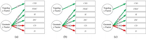
Figure A1. Path diagrams of the OnonR4D Model: (a) OnonR4D-6; (b) OnonR4D-7; (c) OnonR4D-8. The green and red arrow indicate the positive and negative, respectively, and the number on each of arrows represent the absolute value of the influence coefficients of the principal components of the OnonR4D-6/7/8 model (similarly hereinafter).

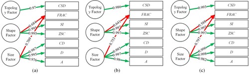
Figure A2. Path diagrams of the OR4D Model: (a) OR4D-6; (b) OR4D-7; (c) OR4D-8.

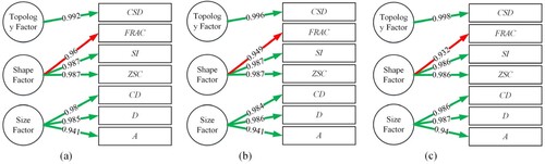
Figure A3. Path diagrams of the InonR4D Model: (a) InonR4D-6; (b) InonR4D-7; (c) InonR4D-8.

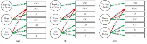
Figure A4. Path diagrams of the IR4D Model: (a) IR4D-6; (b) IR4D-7; (c) IR4D-8.

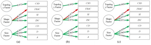
Figure A5. Path diagrams of the ISEA4D Model: (a) ISEA4D-6; (b) ISEA4D-7; (c) ISEA4D-8.

References

- Ali, Mahdavi-Amiri, Alderson Troy, and Samavati Faramarz. 2015. “Data Management Possibilities for Aperture 3 Hexagonal Discrete Global Grid Systems.” ISPRS International Journal of Geo-Information 4 (1): 320–336. doi:10.3390/ijgi4010320
- Ben, Jin. 2005. “A Study of the Theory and Algorithms of Discrete Global Grid Data Model for Geospatial Information Management.” [In Chinese.] PhD diss. The Information Engineering University.
- Bousquin, Justin. 2021. “Discrete Global Grid Systems as Scalable Geospatial Frameworks for Characterizing Coastal Environments.” Environmental Modelling & Software 146: 105210–105224. doi:10.1016/j.envsoft.2021.105210
- Bowater, D., and E. Stefanakis. 2018. “The rHEALPix Discrete Global Grid System: Considerations for Canada.” Geomatica 72 (1): 27–37. doi:10.1139/geomat-2018-0008
- Breunig, Martin, Patrick Erik Bradley, Markus Jahn, Paul Kuper, Nima Mazroob, Norbert Rösch, Mulhim Al-Doori, Emmanuel Stefanakis, and Mojgan Jadidi. 2020. “Geospatial Data Management Research: Progress and Future Directions.” ISPRS International Journal of geo-Information 9 (2): 95–115. doi:10.3390/ijgi9020095
- Bush, I. 2017. "OpenEAGGR - Open Equal Area Global GRid". Accessed Jun 18, 2022. https://github.com/riskaware-ltd/open-eaggr
- Chen, Jun, Hao Wu, and Songnian Li. 2017. “Research Progress of Global Land Domain Service Computing: Take GlobeLand30 as an Example.” [In Chinese.] Acta Geodaetica et Cartographica Sinica 46 (10): 1526–1533. doi:10.11947/j.AGCS.2017.20170411.
- Engwirda, Darren, and Chang Liao. 2021. “'Unified’ Laguerre-Power Meshes for Coupled Earth System Modelling.” Paper presented at the Meeting of 29th International Meshing Roundtable (IMR), Virtual Conference, October 9.
- Gibb, R. G. 2016. “The rHEALPix Discrete Global Grid System.” IOP Conference Series Earth and Environmental Science 34 (1): 1–21. doi:10.1139/geomat-2018-0008.
- Goodchild, Michael F. 2018. “Reimagining the History of GIS.” Annals of GIS 24 (1): 1–8. doi:10.1080/19475683.2018.1424737
- Gregory, Matthew J., A. Jon Kimerling, Denis White, and Kevin Sahr. 2008. “A Comparison of Intercell Metrics on Discrete Global Grid Systems.” Computers, Environment and Urban Systems 32 (3): 188–203. doi:10.1016/j.compenvurbsys.2007.11.003
- Heikes, Ross, and David A. Randall. 1995. “Numerical Integration of the Shallow Water Equations on Twisted Icosahedral Grid Part II a Detailed Description of the Grid and an Analysis of Numerical Accuracy.” Monthly Weather Review 123 (6): 1881–1887. https://doi.org/10.1175/1520-0493(1995)123<1881:NIOTSW>2.0.CO;2
- Hojati, Majid, and Colin Robertson. 2020. “Integrating Cellular Automata and Discrete Global Grid Systems: A Case Study Into Wildfire Modelling.” AGILE: GIScience Series 1 (6): 1–23. doi:10.5194/agile-giss-1-6-2020
- Hojati, Majid, Colin Robertson, Steven Roberts, and Chiranji Chaudhuri. 2022. “GIScience Research Challenges for Realizing Discrete Global Grid Systems as a Digital Earth.” Big Earth Data 6 (3): 358–379. doi:10.1080/20964471.2021.2012912
- Jendryke, Michael, and Stephen C. Mcclure. 2019. “Mapping Crime-Hate Crimes and Hate Groups in the USA: A Spatial Analysis with Gridded Data.” Applied Geography 111: 102072–102082. doi:10.1016/j.apgeog.2019.102072
- Jendryke, Michael, and Stephen C. Mcclure. 2021. “Spatial Prediction of Sparse Events Using a Discrete Global Grid System: A Case Study of Hate Crimes in the USA.” International Journal of Digital Earth 14 (6): 789–805. doi:10.1080/17538947.2021.1886356
- Kimerling, A. J., K. Sahr, and D. White. 1999. “Comparing Geometrical Properties of Global Grids.” Cartography and Geographic Information Science 26 (4): 271–288. doi:10.1559/152304099782294186
- Kmoch, Alexander, Ivan Vasilyev, Holger Virro, and Evelyn Uuemaa. 2022. “Area and Shape Distortions in Open-Source Discrete Global Grid Systems.” Big Earth Data 6 (3): 256–275. doi:10.1080/20964471.2022.2094926
- Li, Xidong, Zhixing Guo, Nanrong Deng, and Ya Wen. 2007. “Analysis of Spatial Variability for the Fractal Dimension and Stability Indexes of Land use Type.” [In Chinese.] Ecology and Environmental Sciences 16 (2): 627–631. doi:10.16258/j.cnki.1674-5906.2007.02.071.
- Liao, Chang, Teklu Tesfa, Zhuoran Duan, and L. Ruby Leung. 2020. “Watershed Delineation on a Hexagonal Mesh Grid.” Environmental Modelling and Software 128: 104702. doi:10.1016/j.envsoft.2020.104702
- Liao, Chang, Tian Zhou, Donghui Xu, Richard Barnes, Gautam Bisht, Hong-Yi Li, Zeli Tan, et al. 2022. “Advances in Hexagon Mesh-Based Flow Direction Modeling.” Advances in Water Resources 160: 104099. doi:10.1016/j.advwatres.2021.104099
- Liao, Chang, Tian Zhou, Donghui Xu, Matthew G. Cooper, Darren Engwirda, Hong-Yi Li, and L. Ruby Leung. 2023. “Topological Relationship-Based Flow Direction Modeling: Mesh-Independent River Networks Representation.” Journal of Advances in Modeling Earth Systems 15 (2): e2022M–e3089M. doi:10.1029/2022MS003089.
- Liao, Chang, Tian Zhou, Donghui Xu, Zeli Tan, Gautam Bisht, Matthew G. Cooper, Darren Engwirda, Hongyi Li, and L. Ruby Leung. 2022. “Topological Relationship-Based Flow Direction Modeling: Stream Burning and Depression Filling.” Authorea Preprints.
- Lin, Bingxian, Liangchen Zhou, Depeng Xu, A. Xing Zhu, and Guonian Lu. 2018. “A Discrete Global Grid System for Earth System Modeling.” International Journal of Geographical Information Science 32 (4): 711–737. doi:10.1080/13658816.2017.1391389
- Liu, Guangxing. 2013. “Data Integration of China Ocean Tidal Wave Based on Spherical Diamond Grid.” [In Chinese.] MA diss. Jiangxi University of Science and Technology.
- Lu, Fuqiang. 2016. “A Finite Volume Model for Global two-Dimensional Ocean Tides on Spherical Block-Structed Qudrilateral Grids.” [In Chinese.], PhD diss., Nanjing Normal University.
- Ma, Yue, Guoqing Li, Xiaochuang Yao, Qianqian Cao, Long Zhao, Shuang Wang, and Lianchong Zhang. 2021. “A Precision Evaluation Method for Remote Sensing Data Sampling Based on Hexagon Discrete Grid.” ISPRS International Journal of Geo-Information 10 (3): 194–215. doi:10.3390/ijgi10030194
- Ming, Tao, Dafang Zhuang, Wen Yuan, Dongsheng Qiu, and Zhangang Wang. 2007. “The Study on the Geometrical Homogenization of Discrete Global Grid Model.” [In Chinese.] High Technology Letters 17 (8): 845–851. doi:10.3321/j.issn:1002-0470.2007.08.015.
- Neeraj, Sirdeshmukh, Edward Verbree, Peter Van Oosterom, Stella Psomadaki, and Martin Kodde. 2019. “Utilizing a Discrete Global Grid System for Handling Point Clouds with Varying Locations, Times, and Levels of Detail.” Cartographica: The International Journal for Geographic Information and Geovisualization 54 (1): 4–15. doi:10.3138/cart.54.1.2018-0009
- Purss, Matthew B. J., Steve Liang, Robert Gibb, Faramarz Samavati, Perry Peterson, Clinton Dow, Jin Ben, and Sara Saeedi. 2017. “Applying Discrete Global Grid Systems to Sensor Networks and the Internet of Things.” Paper presented at the meeting of IEEE international geoscience and remote sensing symposium (IGARSS), July 23-28.
- Purss, Matthew B. J., Perry R. Peterson, Peter Strobl, Clinton Dow, and Jin Ben. 2019. “Datacubes: A Discrete Global Grid Systems Perspective.” Cartographica The International Journal for Geographic Information and Geovisualization 54 (1): 63–71. doi:10.3138/cart.54.1.2018-0017
- Rawson, Andrew, Zoheir Sabeur, and Mario Brito. 2022. “Intelligent Geospatial Maritime Risk Analytics Using the Discrete Global Grid System.” Big Earth Data 6 (3): 294–322. doi:10.1080/20964471.2021.1965370
- Robertson, Colin, Chiranjib Chaudhuri, Majid Hojati, and Steven A. Roberts. 2020. “An Integrated Environmental Analytics System (IDEAS) Based on a DGGS.” ISPRS Journal of Photogrammetry and Remote Sensing 162 (4): 214–228. doi:10.1016/j.isprsjprs.2020.02.009
- Sahr, K. 2019. “DGGRID version 7.0.” Accessed 18, 2022. https://www.discreteglobalgrids.org/software/.
- Sahr, Kevin, Mark Dumas, and Neal Choudhuri. 2015. “The PlanetRisk Discrete Global Grid System.” Accessed November 15, 2018.
- Sahr, Kevin, and Denis White. 1998. “Discrete Global Grid Systems". Computer Science and Statistics (SERIES). po box 7460, Fairfax, VA 22039-7460 USA. May 13-16. 269-278.
- Sun, Wenbin, and Changjiang Zhou. 2016. “A Method of Constructing Approximate Equal-Area Diamond Grid.” [In Chinese.] Geomatics and Information Science of Wuhan University 41 (8): 1040–1045. doi:10.13203/j.whugis20140397.
- Thompson, Jeffery A., Mary J. Brodzik, Kevin A. T. Silverstein, Mason A. Hurley, and Nathan L. Carlson. 2022. “EASE-DGGS: A Hybrid Discrete Global Grid System for Earth Sciences.” Big Earth Data 6 (3): 340–357. doi:10.1080/20964471.2021.2017539
- Uber, Technologies. Inc. 2019. "H3: Hexagonal Hierarchical Geospatial Indexing System". Accessed Jun 18, 2022. https://github.com/uber/h3
- Veach, E., J. Rosenstock, E. Engle, and T. Manshreck. 2017"S2 Geometry Library: Computational geometry and spatial indexing on the sphere". Accessed Jun 18, 2022. https://s2geometry.io
- Wang, Ning, and Jin Luen Lee. 2011. “Geometric Properties of the Icosahedral-Hexagonal Grid on the Two-Sphere.” Society for Industrial and Applied Mathematics 33 (5): 2536–2559. doi:10.1137/090761355.
- Wang, Zheng, Xuesheng Zhao, Wenbin Sun, Fuli Luo, Yalu Li, and Yuanzheng Duan. 2021. “Correlation Analysis and Reconstruction of the Geometric Evaluation Indicator System of the Discrete Global Grid.” ISPRS International Journal of Geo-Information 10 (3): 115–143. doi:10.3390/ijgi10030115
- White, Denis, A. Jon Kimerling, Kevin Sahr, and Lian Song. 1998. “Comparing Area and Shape Distortion on Polyhedral-Based Recursive Partitions of the Sphere.” International Journal of Geographical Information Systems 12 (8): 805–827. doi:10.1080/136588198241518
- Yao, Xiaochuang, Guoqing Li, Junshi Xia, Jin Ben, Qianqian Cao, Long Zhao, Yue Ma, Lianchong Zhang, and Dehai Zhu. 2020. “Enabling the Big Earth Observation Data via Cloud Computing and DGGS: Opportunities and Challenges.” Remote Sensing 12 (1): 62–77. doi:10.3390/rs12010062
- Yuan, Zhengyi, Xuesheng Zhao, and Jing Zhao. 2018. “An Approximate Equal-Area Diamond Mesh Model Based on Latitude-Ring Method and Triangle Aggregation.” [In Chinese.] Bulletin of Surveying and Mapping 0 (1): 107–111. doi:10.13474/j.cnki.11-2246.2018.0020
- Zhang, Bin, Zhengyi Yuan, Xuesheng Zhao, and Xinjian Zhang. 2015. “An Geometry Deformation Evaluation Index of the Spherical Discrete Grid Based on the Fuzzy Similarity.” [In Chinese.] Geography and Geo-Information Science 31 (5): 20–24. doi:10.3969/j.issn.1672-0504.2015.05.005
- Zhao, Xuesheng, and Bai Jianjun. 2007. “Hierarchical Model of Global Discrete Grids Based on Diamonds.” [In Chinese.] Journal of China University of Mining & Technology 36 (3): 397–401. doi:10.3321/j.issn:1000-1964.2007.03.025
- Zhao, Xuesheng, Wenbin Sun, and Jun Chen. 2005. “Distortion Distribution and Convergent Analysis of the Global Discrete Grid Based on QTM.” [In Chinese.] Journal of China University of Mining & Technology 34 (4): 438–442. doi:10.3321/j.issn:1000-1964.2005.04.007
- Zhao, Xuesheng, Zhengyi Yuan, Longfei Zhao, and Sikun Zhu. 2016. “An Improved QTM Subdivision Model with Approximate Equal-Area.” [In Chinese.] Acta Geodaeticaet Cartographica Sinica 45 (1): 112–118. doi:10.11947/j.AGCS.2016.20140598
- Zhou, Qiming. 2001. “Reference Model of Digital Earth.” In [In Chinese.] in from Digital Image to Digital Earth, edited by Denren Li, 88–95. Wuhan: Wuhan University of Surveying and Mapping Press.
- Zhou, Jianbin, Jin Ben, Rui Wang, Mingyang Zheng, Xiaochuang Yao, and Lingyu Du. 2020. “A Novel Method of Determining the Optimal Polyhedral Orientation for Discrete Global Grid Systems Applicable to Regional-Scale Areas of Interest.” International Journal of Digital Earth 13 (12): 1553–1569. doi:10.1080/17538947.2020.1748127
- Zhou, Liangchen, Wenjie Lian, Guonian Lv, A. Xing Zhu, and Bingxian Lin. 2018. “Efficient Encoding and Decoding Algorithm for Triangular Discrete Global Grid Based on Hybrid Transformation Strategy.” Computers, Environment and Urban Systems 68 (2): 110–120. doi:10.1016/j.compenvurbsys.2017.11.005
- Zhou, Chenghu, Yang Ou, and Ting Ma. 2009. “Progresses of Geographical Grid Systems Researches.” [In Chinese.] Progress in Geography 28 (5): 657–662. doi:10.11820/dlkxjz.2009.05.002